A C susceptibility as a probe of low frequency magnetic dynamics

magnetic dynamics

C. V. Topping_‡and S. J. Blundell

University of Oxford, Department of Physics, Clarendon Laboratory, Parks Road, Oxford OX1 3PU, United Kingdom

Abstract. The experimental technique of a.c. susceptibility can be used as a probe of magnetic dynamics in a wide variety of systems. Its use is restricted to the low-frequency regime and thus is sensitive to relatively slow processes. Rather than measuring the dynamics of single spins, a.c. susceptibility can be used to probe the dynamics of collective objects, such as domain walls in ferromagnets or vortex matter in superconductors. In some frustrated systems, such as spin glasses, the complex interactions lead to substantial spectral weight of fluctuations in the low-frequency regime, and thus a.c. susceptibility can play a unique role. We review the theory underlying the technique and magnetic dynamics more generally and give applications of a.c. susceptibility to a wide variety of experimental situations.

1. Introduction

The measurement of d.c. magnetic susceptibility is commonly used to characterise a newly discovered magnetic material. Such a measurement can allow the elucidation of various magnetic properties of materials such as the presence of a phase transition, the magnetic moment of a material or simply the sign of magnetic exchange. However, in a d.c. measurement, the assumption is made that the sample properties remain effectively static, so that there is no measurable dynamic response. This assumption can be restated in terms of the dynamics being much faster, or slower, than the experimental timescale. While this assumption holds in many cases, there are many classes of material where it does not. In such cases, much useful information can be gained by employing a.c. magnetic susceptibility, a technique which utilises a periodic magnetic field rather than a static d.c. magnetic field. A.c. magnetic susceptibility has found application in various areas such as molecular magnetism [1, 2], ferromagnetism [3] and superconductivity [4, 5] and may be used to help differentiate between different types of slow relaxation [1, 6, 7, 8] and derive energy barriers for that relaxation [1, 2, 3].

In this paper, we aim to provide a unified description of a.c. susceptibility. We first contrast the a.c. and d.c. techniques in section 2 and then, in section 3, introduce a.c. susceptibility within the framework of linear response theory, highlighting similarities and differences with dielectric relaxation. We outline methods of modelling real a.c. susceptibility data and illustrate these approaches with their applications to various classes of material in section 4.

2. D.C. and A.C. Magnetic Susceptibility

Magnetic susceptibility,χ, is defined by the equation

χ= lim

H→0 M

H, (1)

where M is the sample magnetisation and H is the applied magnetic field. It is sometimes defined as a differential susceptibility

χ= ∂M

∂H. (2)

In the (commonly encountered) cases when χ 1, B=µ0(H+M)'µ0H, and so

χ_' lim

B→0 µ0M

B . (3)

These equations apply to both d.c. and a.c magnetic susceptibility. However, in a real experiment for the signal to be measurable we require the applied field to be of sufficient strength to produce that signal, and so the limit of vanishing field cannot be achieved. Since M generally is not linear with H and susceptibility can be field dependent, one can define the differential susceptibility

χexp = δM δH 'µ0

δM

δB, (4)

whereδB=µ0δHis a finite applied magnetic field.

2.1. D.C. Susceptibility

For a d.c. measurement, δB is a small, static d.c. magnetic field (typically in the range 0.001–0.1 T, though values outside this can be used) and the resulting magnetization δM is recorded. Typically, d.c. magnetic susceptibility of a system is measured as a function of temperature in two separate warming cycles. First, the sample will be cooled in zero applied magnetic field before applying the measurement field δB and measuring δM(T) at a number of fixed temperatures on the first warming cycle. This is the zero field cooled (ZFC) sweep and the data recorded in this sweep probe the system taken out of steady state conditions. Second, the sample is re-cooled but this time with the measurement fieldδBand the warming cycle of measurements is repeated. This yields the field cooled (FC) sweep and the data recorded correspond to the system in the steady state. Thus, measurement of FC and ZFC sweeps can give an indication of the presence of slow magnetic relaxation, but the relevant timescale that is being probed depends on the rate at which both the magnet can be swept and a measurement can be made (if the dynamics are faster than this, the ZFC and FC sweeps will be identical). Nevertheless, d.c. susceptibility remains a powerful tool for material study.

a sample held at a constant temperature [9]. This can be referred to as d.c. relaxation, remanence orM(t)

dependence and is useful when the relaxation time is several tens of seconds, or even several hours, but is difficult to measure when the relaxation time is shorter than time needed to remove the magnetic field.

2.2. A.C. Magnetic Susceptibility

In a.c. magnetic susceptibility, a time varying, sinusoidal magnetic field of amplitudeHa.c.(typically

∼0.5mT, though other values can be used) is applied to the sample. Simultaneously, a static, d.c. magnetic field (Hd.c.) may also be applied, though often this is set to zero (and the a.c. measurement is then directly probing the ground state of the spin system due to the small a.c. amplitude). Thus the fieldH inside the sample is given by

H =Hd.c.+Ha.c.cos(ωt), (5)

where ω (= 2πν) is the frequency of the oscillating magnetic field. The frequency ν is typically in the range 0.1–104_{Hz and so probes processes which are} faster than those studied by the magnetic relaxation technique described above. In this paper we will restrict our discussion to the situation in which the a.c. and d.c. magnetic fields are applied in parallel. The oscillating response of the magnetisation is recorded (Ma.c.) and the a.c. susceptibility is then defined by

χa.c.= Ma.c. Ha.c.

. (6)

This equation has assumed that the response of the system is linear so that Ma.c. is proportional to Ha.c. with the constant of proportionality χa.c.; this is however not always the case and we will consider such nonlinear response in section 3.7.

3. Theory and models

In this section we will consider the theoretical background to measurements of a.c. susceptibility. Before considering linear response in section 3.2, we will in section 3.1 provide a physical motivation for the relationship between the frequency ω and the characteristic relaxation time τ of the system. In sections 3.3–3.5 we will explore various models of a.c. susceptibility, as well as ways of representing the response in the complex plane in section 3.6. Non-linear effects will be considered in section 3.7 and then in section 3.8 we will describe the workings of a practical susceptometer.

M

H

2Ha.c.

Figure 1. Graphical demonstration of the use of a.c. magnetic susceptibility for measurement of the gradient of a magnetisation curve. The red dashed line demonstrates the gradient being measured and the blue dotted line shows the applied d.c. magnetic field which can be changed to allow different parts of the magnetisation curve to be investigated.

10-410-2 1 102 104 106 108101010121014

(Hz)

104 102 1 10-210-410-610-810-1010-1210-14 -1

(s)

A.C. Susceptibility

Remanent Magnetisation NMR SR

Perturbed Angular Correlations

Mossbauer Neutron Scattering

Figure 2. Comparison of approximate frequency ranges available to various experimental techniques. Information gathered from references [10, 11]. Note that (following equation (24))χ00has a maximum whenωτ= 1and so this occurs atτ=ν−1_{/2πand the}

factor of1/2πshould not be forgotten.

3.1. Three characteristic regimes

Depending on the relaxation time τ of the magnetic moments of the studied system, three regimes can be defined on the basis of the relative sizes ofωand1/τ.

system responds essentially instantaneously to the a.c. field and d.c. susceptibility is obtained (χa.c.≈χd.c.). This is an equilibrium response and the moments are able to exchange energy with the lattice. This results in a measurement of what we can call the isothermal susceptibility, χT [1]. Given the increased sensitivity that may be achieved due to measuring an oscillating response, a.c. susceptibility may be useful in studying systems where dynamics are not being considered but the signal is weak. Furthermore, when using susceptibility as a measurement of the gradient ofM versus H, the ability to apply a d.c. magnetic field allows different regions of the M versus H curve to be probed as shown in figure 1.

(2)ω1/τ: The second regime occurs when the perturbing field oscillates too quickly for the magnetic moments of the system to respond. Thus the system does not have time to equilibrate and exchange energy with the lattice. The obtained susceptibility is known as the adiabatic susceptibility,χS [1].

(3) ω _≈ 1/τ: The intermediate regime, in which the frequency of the oscillating magnetic field is comparable to the timescale of the magnetic relaxation of the system, offers a much more complex response. In this regime there may be some phase lag (and therefore dissipation) when the perturbation is slightly faster or slower than the natural frequency of the system. Thus, the response is reported in two parts: in-phase and out-of-phase (or real and imaginary) components respectively, M0

a.c. and M00

a.c., with corresponding susceptibility,χ0a.c.andχ00a.c.. As shown below, the imaginary component relates to dissipation in the system. The a.c. magnetic susceptibility may be written as a complex number

χa.c.=χ0a.c.+iχ

00

a.c., (7)

which at low and high frequency must reduce to the real value (χ00

a.c. = 0) of χT or χS respectively. For brevity, the subscript “a.c.” will be neglected from this point onward. The choice of the sign of the imaginary part of the susceptibility in equation (7) is a matter of convention. In some treatments, the complex susceptibility is defined instead asχ0−iχ00, and we will switch to this alternative choice later in this paper (in Section 3.4).

Ideally, when choosing a technique to examine dynamic behaviour frequencies that allow the prob-ing of all three regimes should be available. Fig-ure 2 shows a comparison of several experimental techniques demonstrating both that a.c. magnetic sus-ceptibility probes the lower frequency region and over-lap does exist between techniques which can be taken advantage of should a system’s characteristic time be at the edge of the available frequency region.

Descriptions of slow magnetic relaxation typically use a form known as the generalised Debye model.

This has found application in various systems including single-molecule magnets [1], spin glasses [8] and ferromagnets [3]. This model was originally derived and applied to dielectric systems [12, 13, 14], though also arose in treatments of magnetic materials [15, 16]. Our approach will be to use linear response theory, outlined in Section 3.2, and to show how it may lead to the generalised Debye model and other related models in the sections that follow.

3.2. Linear response theory

An arbitrary system will show a generalised displace-ment,x(t), as a result of a generalised force,f(t). The value ofxat timetis then given by

x(t) =

Z ∞

−∞

χ(t−t0)f(t0)dt0, (8) whereχ(t₋t0_{)is a generalised response function. This}

relation is a convolution and hence we can write it as a product,

˜

x(ω) = ˜χ(ω) ˜f(ω), (9)

by using the Fourier transform of x(t), χ(t)andf(t), explicitly defined as

˜

x(ω) =

Z ∞

−∞

e−iωt_{x(t)dt; (10)}

x(t) =

Z ∞

−∞ 1 2πe

iωt_{x˜(ω)dω. (11)}

To simplify notation, we will drop the tildes on Fourier transforms and write them as x(ω), f(ω), χ(ω), etc. Furthermore, we will assume that χ(t₋t0_{) = 0 for}

t < t0 _{(an assumption of causality) and hence we}

can writeχ(t) =X(t)θ(t)whereθ(t)is the Heaviside step function. The function X(t) = χ(t) for t > 0, but can take any value for t < 0, so let us set it to X(t) =₋χ(_|t_|)fort <0, makingX(t)an odd function (and henceX(ω)is purely imaginary). Then

χ(ω) = 1 2π

Z ∞

−∞

θ(ω0

−ω)X(ω)dω0_{, (12)}

and usingθ(ω) =πδ(ω)₋i/ω, we have

χ(ω) = 1 2X(ω)−

i

2πP

Z ∞

−∞

X(ω0₎

ω0_−ωdω

0_=χ0_(ω)+iχ00_(ω),

(13) where χ0 _{and χ}00 _{are the real and imaginary parts of}

χ(ω) and P indicates that the Cauchy principal value is taken to avoid a singularity. BecauseX(ω)is purely imaginary, equation 13 implies that

iχ00(ω) = 1

and

χ0(ω) =P

Z ∞

−∞ dω0 χ

00_(ω0₎

π(ω0_−ω). (15)

Equation (15) is one of the Kramers-Kronig relations which connects the real and imaginary parts of the response functions. Atω = 0 equation (15) reduces to

πχ0(0) =P

Z ∞

−∞ dω0χ

00_(ω0₎

ω0 . (16)

The quantityχ0_{(0)is called the static susceptibility.}

3.3. The damped harmonic oscillator

A damped harmonic oscillator serves as an example of this approach. The equation of motion is given by

mx¨+αx˙+kx=f, (17)

wheremis the mass,αis the damping constant andk is the spring constant. Writing the resonant frequency, ω2

0 =k/m, and damping,γ=α/m, we have

χ(ω) =x(ω)

f(ω) = 1

m

1

ω2

0−ω2−iωγ

. (18)

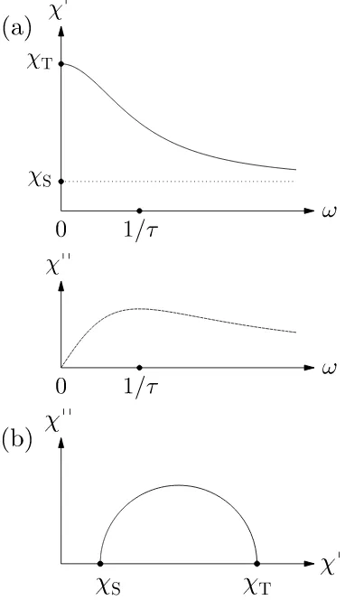
This is a complex function and the real and imaginary parts are plotted in figure 3(a). The imaginary part χ00_{(ω)is given explicitly by}

χ00(ω) = ωγ/m

(ω2_−ω2

0)2+ (ωγ)2

. (19)

The static susceptibility is χ0_{(0) = 1/mω}2

0 = 1/k, and straightforward integration shows that the sum-rule in equation (16), R∞

−∞χ

00_{(ω)/ωdω = πχ}0_{(0), is}

satisfied; this relation is shown in figure 3(b). For later reference, we also show a plot of χ00 _againstχ0 _{in an}

Argand diagram in figure 3(c).

Now we remove the inertial term resulting in the equation of motion becoming

αx˙+kx=f (20)

with

χ(ω) = 1/k

1₋iωτ, (21)

whereτ =α/k. This yields real and imaginary parts

χ0(ω) = 1/k 1 +ω2_τ2;

χ00_{(ω) =} ωτ /k

1 +ω2_τ2. (22)

Moreover, it is common to include an additive adiabatic response,χS, so that

χ(ω) =χS+

1/k

1₋iωτ. (23)

Figure 3. (a) The real and imaginary parts of χ as a function of ω. (b) Illustration of equation (16) for the damped harmonic oscillator. (c) The same curves as in panel (a) but plotted in an Argand diagram.

Thus in the case of a.c. susceptibility, this expression becomes

χ0(ω) =χS+

(χT −χS)

1 +ω2_τ2 ;

χ00_{(ω) =} (χT −χS)

1 +ω2_τ2 ωτ, (24)

where we have written χT = χS + 1/k. HereχS = χ(_∞)is the adiabatic susceptibility andχT = χ(0) is the isothermal susceptibility. These equations recover the required limits at high and low frequencies, namely a reduction of χ0 _{to adiabatic and isothermal values}

respectively, as well as a vanishing of χ00 _{at both}

Figure 4.(a) The real and imaginary parts ofχas a function ofωfor the model with no inertial term. The maximum inχ00occurs when

ωτ = 1, i.e. atω = 1/τ. (b) The same curves as in panel (a) but plotted in an Argand diagram (known as a Cole-Cole plot).

as a function of ω (on a linear scale; to see these curves on a logarithmic scale of ω, see the α = 0

curves in figure 5(a) and (d) below). Perhaps the most important feature present is the maximum ofχ00_which

occurs at ωτ = 1 providing a convenient method to extract the relaxation time of a system. In this model, the solution for equation (20) with f = 0 (τ _≥ 0) is given by

x(t) =x(0)e−t/τ ₍₂₅₎

and describes a relaxation process with a single relaxation time. For a magnetic system,x(t)becomes M(t), so that if a system has a magnetization which relaxes exponentially with time then it can be described by equation (24). If χ00 _{is plotted against}

χ0in the Argand diagram, a characteristic semicircular form is produced as shown in figure 4(b).

3.4. Dielectric relaxation

The model we have been considering (summarised in equation (23)) is analogous to the well-known

expression for dielectric relaxation described in the Debye model [14]. In Debye’s treatment, the generalised displacement becomes the electric polarisation, P(t), and the generalised force is an electric field, E(t). The model is usually formulated in terms of the relative permittivity (ω) = 1 +

P(ω)/(0E(ω)). Then, in the notation conventionally used to describe dielectric relaxation

0 ₌ ∞+

S−∞ 1 +ω2_τ2;

00₌ωτ(S−∞)

1 +ω2_τ2 , (26) whereSis the static permittivity (=T, the isothermal permittivity in the language we have adopted) and∞

is the permittivity in the high-frequency limit (= S, the adiabatic permittivity in the language we have adopted).

Many of the treatments of a.c. susceptibility borrow expressions used in dielectric relaxation, and in the field of dielectric relaxation it is conventional to write the complex susceptibility in the Debye model as

χ(ω) =χS+

χT −χS

1 +iωτ , (27) where the sign difference in the denominator occurs due to the previously mentioned differing convention of complex susceptibility (which is defined as χa.c. = χ0

− iχ00 _{for the above equation). We will use}

this convention from now on as it is the usual choice in the literature. Both equations (23) and (27) lead to the same real and imaginary parts of equations (24) (equivalent to the dielectric case given in equation (26)).

The Debye model fails to model short times (and thus high frequencies) and violates the sum-rule that R∞

0 ωχ

00_{(ω) dω should remain finite, so}

modifications sometimes need to be considered if very high-frequency studies are carried out [17] which, for example, can be done using time-domain terahertz spectroscopy [18].

3.5. A range of relaxation times

the case of magnetism, the limit of completely non-interacting magnetic moments also seems unlikely to be encountered due to the presence of cooperative ef-fects, though it might not necessarily be a bad approx-imation for systems such as superparamagnets [21] or single-molecule magnets [1].

In order to account for these complexities, several approaches can be employed. One strategy is to introduce a spread of relaxation times into the model. This is often accounted for by introducing a phenomelogical parameterαinto what is then called the generalised Debye model

χ(ω) =χS+

χT −χS

1 + (iωτ)1−α, (28) where0 ≤α ≤1[1, 13]. Settingα= 0corresponds to no spread of relaxation times and the ideal Debye model is recovered. This modification (shown in figures 5(a) and (d)) is successful in describing slowly relaxing electric [13] and magnetic systems [1, 2, 22, 23]. An alternative approach is known as the Cole-Davidson model (shown in figures 5(b) and (e)) [24] which instead places an exponent β in the denominator as follows:

χ(ω) =χS+

χT −χS

(1 +iωτ)β. (29)

In the study of dielectric systems these equations are sometimes combined to produce the Havriliak-Negami equation

χ(ω) =χS+

χT −χS

[1 + (iωτ)1−α_]β, (30) which (by virtue of introducing two variable parame-ters) can improve the agreement with data from real systems [25, 26]. Plots of this model with various parameter values are shown in figures 5(c) and (f). However, the introduction of additional fitting vari-ables risks overparameterization.

Each of the above extensions of the Debye model (equations (28)–(30)) are all somewhat ad hoc adjustments introduced to yield improved agreement between real systems and theory (for example, reference [24] refers to the Cole-Davidson model as an empirical formula). Therefore, their use which will be shown for single-molecule magnets, spin glasses and spin ices in Sections 4.2, 4.3 and 4.4 respectively tends to arise because of the typical models employed in these areas. Common to each of these extensions is the assumption that a single relaxation time no longer governs the system dynamics, with a distribution of relaxation times parameterised by α and/or β, depending on the model used. The effect of multiple relaxation times can be illustrated by considering a magnetic system composed of two magnetic entities

with distinct relaxation times τ1 and τ2. The total magnetisation of the system is then the sum of each entity’s magnetisation, and so the susceptibilities will also add. Hence

χ=χ1+χ2=

χS,1+

χT ,1−χS,1

1 +iωτ1

+χS,2+

χT ,2−χS,2

1 +iωτ2

. (31)

If each entity has the same magnetic moment andη is the fraction of the system composed of the first entity and1₋η the fraction composed of the second entity this reduces to

χ=χS+ (χT −χS)

η

1 +iωτ1

+ 1−η 1 +iωτ2

, (32)

where we have assumed each entity relaxes exponen-tially in a Debye-like manner. (A similar approach is used in reference [19], with a different definition of constants.) This model gives two maxima in χ00 _at

ω = 1/τ1 andω = 1/τ2which are easy to distinguish if there is a large enough separation between the two relaxation times. This approach however retains the limitations intrinsic in the Debye model (such as the neglect of interactions). Some simulations based on the model of equation (32) (for which the two time constants are assumed to be separated by a factor of one hundred) are shown in figure 6. This demonstrates the two maxima inχ00_{and also shows how two arcs are}

generated in the Cole-Cole plot; Cole-Cole plots under-going further discussion in the next section. Ifτ1and τ2are not too dissimilar, this results in a single asym-metric arc in the Cole-Cole plot [19]. This can look rather similar to the arc produced in the Cole-Davidson model (see figure 5(h)).

This approach can be extended to an arbitrary number of coexisting processes with different relax-ation times. For example, equrelax-ation (32) can be gen-eralised to

χ(ω) =χS+ (χT −χS)

X ηn

1 +iωτn

, (33)

where ηn is the proportion of the system with relaxation time τn and Pηn = 1. If the number of relaxation processes is large, their distribution can be replaced by a continuous function and the summation may be replaced by an integration

χ(ω) =χS+ (χT −χS)

Z τmax

τmin

g(τ)

1 +iωτdτ, (34)

χ

′′

χ

α= 0.0 α= 0.2 α= 0.4 α= 0.6 α= 0.8

χ

′

ωτ

χ

′′

ωτ

χ

′′

χ

β= 1.0 β= 0.8 β= 0.6 β= 0.4 β= 0.2

χ

′

ωτ

χ

′′

ωτ

χ

′′

χ

α= 0, β= 1 α= 0.2, β= 0.8 α= 0.4, β= 0.8 α= 0.4, β= 0.6 α= 0.5, β= 0.5

χ

′

ωτ

χ

′′

ωτ

1

1+(i

ωτ

)

(1+i

1

ωτ

)

1

(1+(i

ωτ

)

)

Figure 5. Example real ((a)-(c)) and imaginary ((d)-(f)) parts of the a.c. response and the Cole-Cole plots ((g)-(i)) for the a.c. magnetic susceptibility interpretation of the Generalised Debye ((a),(d) and (g)), Cole-Davidson ((b), (e) and (h)) and Havriliak-Negami ((c), (f) and (i)) models. These plots assume χS = 0 and χT = 1, though the scaling to general values is obvious. The function

χ(ω) =χS+ (χT−χS)y(ω), wherey(ω)is the function shown at the head of each column in the figure.

The precise form ofg(τ)depends on the system in question. In the case of a single relaxation time τc, g(τ) = δ(τ−τc)and the ideal Debye model with τ = τc is recovered as applicable to systems such as superparamagnets [21] and single-molecule magnets [1]. Various forms of distributions of relaxation times have been considered and are listed in reference [27], though in that work the distribution of relaxation times f(ln(τ)) is defined in terms of the logarithm of the

relaxation time, so that the integral in equation (34) is written asR

d lnτ f(lnτ)/(1 +iωτ)(though the two forms can easily be related using d lnτ = τ−1_{dτ, so} thatτ−1_{f(lnτ) =g(τ)).}

χ

′′

χ′

χ

′

ωτ

χ

′′

ωτ

η= 0.05 η= 0.1 η= 0.25 η= 0.5 η= 0.75 η= 0.95

Figure 6. The real (a) and imaginary (b) parts ofχand the Cole-Cole plot (c) for a model using equation (32) withτ1/τ2 = 100

(τ1=τ,τ2= 0.01τ) and plotted for different values ofη.

[28] is

g(τ) = 1 2πτ

sinαπ

cosh[(1₋α) ln(τ

τc)]−cosαπ

. (35)

Asαapproaches zero, g(τ)gets more sharply peaked nearτ =τc, becomingg(τ) =δ(τ−τc)forα= 0(the ideal Debye model limit). For larger values of αone finds the distribution to be broader.

The same can be done for the Cole-Davidson form χ(ω) =χS+ (χT −χS)/[(1 +iωτc)β](given earlier in equation (29), but note that here we are writing the characteristic time as τc). To do this, following [24] we choose the form ofg(τ)in equation (34) as

g(τ) =



 

 

sinβπ π

1

τ

_τ

τc−τ

β

τ_≤τc

0 τ > τc.

(36)

This function is plotted in figure 7(b) for various values ofβ. As β _→ 1, the function becomes more strongly peaked at τ = τc (and becomes a delta function at β= 1, the ideal Debye model limit). For smaller values of β there is a broader distribution ofτ. In contrast with the generalised Debye model, the distribution has an upper cut-off inτ.

The analogous expressions for the Havriliak-Negami formχ(ω) =χS+(χT−χS)/([1+(iωτc)1−α]β)

(given earlier in equation (30)) is [25, 29, 30]

g(τ) = 1

πτ

τ τc

(1−α)β

sinβΘ

τ τc

2(1−α)

−2τ τc

1−α

cosπα+ 1

β/2,

(37) where

Θ = tan−1

sinπα

τ τc

1−α

−cosπα

. (38)

Equation (37) reduces to equation (35) when β = 1

and to equation (36) whenα= 0.

We note that though these different expressions for g(τ) reproduce the various forms of χ(ω), none of them has an obvious physical basis. One model providing a better fit to experimental data over another can suggest features of the actual distribution function of relaxation times that might be present. For example, a good fit to the Cole-Davidson model might suggest the presence of an upper cut-off in the relaxation time distribution with a long tail, rather than a distribution that is smeared out on either side of τc). However, a distribution of relaxation times could arise from interactions between the relaxing entities and describing this in detail for a real system is a complicated problem, outside the scope of these phenomenological models. In principle, some other contribution of processes could account for the experimental data just as well. The plots in figure 7(a) and (b) are replotted in figure 7(c) and (d), but using a logarithmic time axis (and writingτ−1_{f(ln(τ /τ}

c)) = g(τ)).

Sometimes it is possible to make some statements about a distribution of relaxation times that have a better motivated physical basis. A useful relation that has been applied to spin glasses can be derived by assuming that the distribution of relaxation times is very broad and relatively uniform over several decades, i.e. over a wide range of lnτ; thus let us assume that f(lnτ) = ¯f (where f¯ is a constant) between τmin and τmax, and further that ω lies somewhere in the middle of this range, so thatτmin ω−1

τmax. In this case, using equation (34),χ0 can be written

χ0=χS+ (χT−χS)

Z τmax

τmin

f(τ)

0

1/τc

2/τc

3/τc

g

(

τ

)

τ /τc

(b) Cole-Davidson

β= 0.9

β= 0.8

β= 0.7

β= 0.6

β= 0.5

β= 0.4

β= 0.3

0

1/τc

2/τc

3/τc

g

(

τ

)

τ /τc

(a) Generalized Debye

α= 0.01

α= 0.1

α= 0.2

α= 0.3

α= 0.5

0

1/τc

2/τc

3/τc

f

(l

n

(

τ

/τc

))

ln(τ /τc)

(d) Cole-Davidson

β= 0.9

β= 0.8

β= 0.7

β= 0.6

β= 0.5

β= 0.4

β= 0.3

0

1/τc

2/τc

3/τc

f

(l

n

(

τ

/τc

))

ln(τ /τc)

(c) Generalized Debye

α= 0.01

α= 0.1

α= 0.2

α= 0.3

α= 0.5

Figure 7.The left-hand panels show the form ofg(τ /τc)in (a) the generalized Debye model (plotted for different values ofα) and (b) the

Cole-Davidson model (plotted for different values ofβ). The right-hand panels show the form off(ln(τ /τc))for different values for (c) the

generalized Debye model and (d) the Cole-Davidson model. Thus these are analogous to the plots in panels (a) and (b), but plotted as a function ofln(τ /τc).

and the gradient ofχ0 _{as a function oflnωis}

∂χ0

∂lnω =ω ∂χ0

∂ω (40)

= ₋2(χT−χS) ¯f

Z τmax

τmin

ω2_τ2

1 +ω2_τ2dlnτ (41)

= (χT−χS) ¯f

1 1 +ω2_τ2

max

−_{1 +ω}12_τ2 min

(42)

≈ −(χT−χS) ¯f , (43)

where the last approximation follows from using the limits in the formωτmin1andωτmax1. Similarly, χ00_{can be written}

χ00= (χT−χS)

Z τmax

τmin

f(τ)ωτ

1 +ω2_τ2dlnτ, (44)

= (χT−χS) ¯f[tan−1(ωτmax)−tan−1(ωτmin)] (45)

≈ −(χT−χS) ¯f , (46)

Comparing equations (43) and (46) yields

χ00_≈ π

2

∂χ0

∂lnω, (47)

a relationship between χ0 _{and χ}00_{, first derived by}

Lundgrenet al. [31], that holds quite well in various spin glass systems [32].

3.6. The Cole-Cole plot

χ00=−

χT−χS

2 tan πα 2 ± s _χ

T−χS

2 tan

πα

2

2

+ (χ0_−χ

S)(χT−χ0). (48)

Hereαis a fitting parameter (see, for example, [23]). Equation (48) can be derived from equation (28), as shown in Appendix A. (If a dataset does not extend over a sufficiently large frequency range to carry out this kind of fit, it is still possible to extract α using the angle the data makes with thex-axis in the Cole-Cole plot [13]). In contrast the Cole-Cole-Davidson model (equation (29)) shows a non-symmetric arc in a Cole-Cole plot with one side elongated [24] (see figure 5(h), as well as Appendix B).

In an a.c. susceptibility experiment, the shape of the arcs of a Cole-Cole plot (symmetric for the generalised Debye model and asymmetric for the Cole-Davidson and Havriliak-Negami models) tend to define which model is employed. As such, no particular physical reasoning is usually employed when selecting a model for a system beyond the appearance of the Cole-Cole plot, and so this remains a phenomenological model.

In an ideal situation, an a.c. susceptibility experiment would involve the measurement ofχ0 _and

χ00 _{over a large frequency range so that the condition}

ωτ = 1 is satisfied for every significant relaxation process. In practice, data over a small set of particular frequencies are obtained as temperature is varied due to equipment constraints. If the relaxation time of the system varies with temperature (τ(T)), then for a certain frequency the condition ωτ(T) = 1 may be satisfied at some temperature [1]. Assuming χT andχS vary slowly in this temperature region, a peak will occur in a plot ofχ00 _{vs T when this condition is}

satisfied, for a particular ω, thereby allowingτ(T) to be modelled [1, 2, 33, 34, 35], a point we will return to in Section 4.2.

3.7. Nonlinear effects and harmonics

So far we have considered only linear response, motivated by the definition in equation 2 that states thatM andH are linearly related by χ. However, in general M might be a more complicated function of H, so in that case we can writeM as a polynomial expansion inH[7, 8, 36, 37, 38]:

M =M0+χ(1)H+χ(2)H2+χ(3)H3+. . . (49)

Here M0 is a spontaneous magnetisation (which is zero in several of the systems considered in this paper)

andχ(1) _{is the linear susceptibility that we have been} discussing thus far. If the applied magnetic fieldH is small, then the nonlinear terms can be neglected, but sometimes they need to be considered. Very often only odd powers of H are required in equation (49) due to the symmetry ofM [36, 38, 39], but we will leave them all in. With an applied field given by

H =Ha.c.cos(ωt) (50)

the resultant magnetisationM(t)can be expanded as a Fourier series [8, 40]

M =M0+

∞

X

n=1

Mncos(nωt). (51)

In this case, and assuming that χ(n) _{are all real} quantities, the form of equation (49) yields the following expressions for the Fourier components:

M1=χ(1)Ha.c.+

3 4χ

(3)_H3 a.c.+

5 8χ

(5)_H5 a.c.+· · ·

M2=

1 2χ

(2)_H2 a.c.+

1 2χ

(4)_H4 a.c.+· · ·

M3=

1 4χ

(3)_H3 a.c.+

5 16χ

(5)_H5 a.c.+· · ·

M4=

1 8χ

(4)_H4 a.c.+

3 16χ

(6)_H6 a.c.+· · ·

M5=

3 4χ

(5)_H5

a.c.+· · ·. (52)

The values of these Fourier components will come out differently if the a.c. magnetic field in equation (50) is chosen as a sine, rather than a cosine function (see for example reference [39]). Moreover, more complicated expressions can be derived if a d.c. magnetic field is also applied [39]. Measuring the nonlinear susceptibility has been used to differentiate between different types of slow magnetic relaxation [38] due to the divergence in χ(3) _{near the critical} temperature [8, 37, 41] and can be very sensitive to the presence of some magnetic phases which are undetected in linear a.c. susceptibility [36, 42, 43, 44, 45].

A different treatment of nonlinear effects is used in studies of superconductors, as will be described in section 4.6. There a particular focus is on the real andimaginary parts of the nonlinear susceptibility and explicit forms of the very nonlinear M(H) behaviour according to different models of superconducting behaviour (rather than simply using a series expansion as in equation (49)) can be directly tested [40, 46, 47, 48, 49, 50].

3.8. A.C. Susceptometer

Detection Coils

Sample

A.C. Excitation Coils

D.C. Magnet Coils

D.C. Current Source A.C. Current

Source Lock-In

Amplifier

Reference Cryostat

Electronics

Control Computer

Cryostat

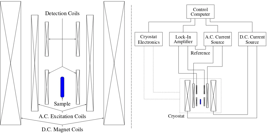
Figure 8. Schematic of the physical apparatus of an a.c. susceptometer. Left shows the set up of the various coils involved in the system. Right shows the electrical connections in an a.c susceptometer.

voltage in a detector/sensing coil (Faraday’s law) and use the magnetisation of a sample to generate this changing flux [51]. For a d.c. measurement a changing magnetic flux is achieved by physically translating the sample through the detection coil [10, 51]. A.c. measurements generate a changing flux due to the applied a.c. magnetic field yielding a time-varying response in the sample with the sample kept stationary. An a.c. susceptometer contains three distinct coil sets: a.c. excitation coils, detector coils, and d.c. magnet coils (see the left panel of figure 8). The a.c. magnetic field is generated by an excitation coil set (sometimes called the primary or drive coils) which are driven by an a.c. current source providing the range of possible frequencies that may be accessed [4, 10, 51, 52]. The detector coils (sometimes called secondary coils) are typically placed within the a.c. excitation coils. They consist of a pair of identical and connected oppositely wound coils with the sample located at the centre of one of these coils [4, 10, 51]. Setting up the system in this way with two detector coils of opposite handedness helps null signals originating form the a.c. field or other external sources by keeping one coil empty [4]. The signal is detected using a lock-in amplifier (taklock-ing a reference from the a.c. current source) thus allowing the in-phase (χ0_{) and}

out-of-phase (χ00_{) components to be detected [4, 52]. Should}

higher harmonics be desired these can be detected using additional lock-in amplifiers at the appropriate multiples of the a.c. drive frequency. This set-up is shown on the right of figure 8.

While the detector coil pair are nominally identical this is normally not perfectly achieved in practice requiring methods to compensate for incomplete nulling [4]. This can be accomplished by including a sample translation stage allowing measurements to be performed with the sample at different positions in the detector coil pair (such as in the centre of the lower detector coil as depicted in figure 8, in the centre of the upper detector coil or between the detector coil) [10]. This is the method adopted by a Quantum Design Physical Property Measurement System using the AC Measurement System option [10]. Accurate determination of the phase difference between the a.c. drive and sample signal is important (noting the in-phase sample signal is actuallyπ/2out-of-phase with the a.c. drive due to Faraday’s law [10]). Any additional phase differences introduced by the electronics must be accounted for [10]. Moreover, the a.c. magnetic field can introduce heating problems at low temperature [10] and mechanical vibrations can affect measurement accuracy [53].

For samples with a large susceptibility, a demag-netization correction should be performed. This is particularly important with a.c. measurements because failure to make an appropriate correction can lead to the real and the imaginary parts being mixed together. Using SI units, the intrinsic susceptibility χ is related to the experimentally measured susceptibilityχexp by χ−1 _{= χ}−1

Therefore the real and imaginary parts are

χ0 = χ 0

exp−N([χ0exp]2+ [χ00exp])

(1−N χ0

exp)2+ (N χ00exp)2

(53)

χ00= χ

00

exp

(1−N χ0

exp)2+ (N χ00exp)2

. (54)

These expressions must be used in studies on superconductors whereχ0

expandχ00expis large.

4. Application to real experimental systems

The models outlined above can describe a wide range of slowly relaxing phenomena. This section provides some examples of various families of experimental systems for which a.c. susceptibility is a useful tool as well as a discussion of the origin of the slow relaxation in each family.

4.1. Paramagnetism

The first magnetic system to consider is paramag-netism. In this state the magnetic moments are free to relax at a rate given by the spin-spin relaxation time which is very fast (i.e. _≈ 10−9

−10−10 _{s) meaning} that the system responds effectively instantaneously, at least on the timescales accessible to a.c. susceptibility [1, 2, 54]. Thus a paramagnet should not show slow relaxation. In fact, χT = χS in a paramagnet which setsχ00 _{= 0according to equation (24). The presence}

of a non-zeroχ00_{can be indicative of a departure from}

paramagnetism. This statement is only true under zero applied d.c. magnetic field. The application of a d.c. field creates a net magnetization and the possibility of spin-lattice relaxation due to direct phonon processes, which are accessible for study using a.c. susceptibility [1].

4.2. Superparamagnets and Single Molecule Magnets

Superparamagnets and single molecule magnets (SMMs) are arguably the simplest systems exhibit-ing slow magnetic relaxation. A superparamagnet describes an assembly of magnetic particles, each of which have sufficiently small physical size that domain wall formation is not possible and the magnetization in each particle becomes a single magnetic domain [1, 21] These are sometimes referred to as magnetic nanoparticles [55, 56, 57]. SMMs (sometimes called zero-dimensional molecular magnets) are a subset of the greater class of molecular magnets [1, 58]. In a SMM, each molecule contains magnetic ions which are linked by organic ligands (an example is shown in fig-ure 9(a) for the molecule Ni12which consists of twelve Ni2+ _{ions and has a S = 12 ground state). The} in-dividual molecules are held together in a crystal only

Figure 9. (a) The single molecule magnet Ni12(chemical formula

[Ni12(chp)12(O2CMe)12(H2O)6(THF)6], where chp = 6-chloro-

2-pyridonate). (b) τ against 1/T measured from ac susceptibility (red circles) or d.c. relaxation (green triangles); inset: χ00_(T)at 10 frequencies. Adapted from reference [61].

rather weakly and each molecule can therefore be con-sidered to be a zero-dimensional magnet (the inter-molecular exchange can largely be neglected) [58]. The intramolecular exchange produces a net “giant spin” ground state (such as the S = 12ground state in Ni12), so that each molecule can be considered as a single, giant magnetic moment to an approximation [1, 59, 60]. Thus SMMs can show superparamagnetic behaviour. The moments in both superparamagnets and SMMs are well isolated from each other and there-fore are good candidates for exhibiting slow relaxation of the kind described by the Debye model.

The source of the slow magnetic relaxation in both systems arises from uniaxial anisotropy (i.e. they contain a magnetic easy axis) making it energetically favourable for moments to align along a specific axis. For superparamagnets, this uniaxial anisotropy arises from magnetocrystalline anisotropy or shape anisotropy and can be described by an energy density

E =Ksin2θ, (55) where K is a constant describing the anisotropy energy density and θ is the angle made with the easy axis by the single domain moment [21, 55]. If K > 0, energy is minimized when the moment is aligned parallel or anti-parallel with the easy axis. Therefore, the potential energy diagram of the magnetic moment is a symmetric double well with an energy barrier separating the parallel and anti-parallel configurations. For SMMs, the anisotropy results from a zero field splitting parameter,D > 0, arising from a Hamiltonian_Hof the form

H=−DSz2+E(S

2

x−S

2

y) +gµBB·S, (56)

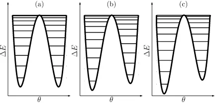
where S is the spin operator, Sx, Sy andSz are the spin components along the x, y and z-axes, E is an additional (rhombic) anisotropy term, g is the g-factor and B is the magnetic field [1, 58, 59, 60]. The term premultiplied by E introduces a medium and hard axis and is essentially a higher order term that we will set to zero for our initial discussion[1]. The symmetric double well potential energy diagram this creates when B = 0 and E = 0 (analogous to superparamagnets) is shown in figure 10(a). The quantized +S and₋S states lie on opposite sides of an energy barrier of height (or activation energy)Ea. (It should be noted that in some papers the parameter D is defined with opposite sign). Slow magnetic relaxation arises from the moments overcoming this energy barrier to change orientation between parallel and anti-parallel states. If this is a thermal process, the relaxation timeτis temperature-dependent and can be described using an Arrhenius law of the form

τ(T) =τ0exp

_E

a kBT

, (57)

where τ0 is known as the inverse attempt frequency (which can be thought of as the time between attempts at thermally exciting over the energy barrier) and can take values down to around 10−11_{s but can} be many orders of magnitude larger [1]. Ea = KV for superparamagnets where V is the volume of the single domain particle [21]. For SMMs, this type of behaviour is associated with a two-phonon Orbach process in which a phonon is absorbed by the spin system, allowing an excited state to be accessed, with the spin system relaxing to its final state, accompanied by the emission of a phonon of a different energy. This allows the spin system to overcome the energy barrier [54, 62]. An experiment such as a.c. susceptibility is carried out at a particular frequency ω, corresponding to a particular time

∆

E

θ

∆

E

θ

∆

E

θ

Figure 10. Potential energy diagram for a system described by the HamiltonianH =−DS2

z with an externally applied magnetic field

ofB= 0((a)),B=D/2gµB((b)) andB=D/gµB((c)). Adapted

from reference [58].

constant τmeasure. As τ(T) sweeps through this time constant as T is lowered, the magnetization changes from dynamic (at high T, where τ(T) τmeasure) to frozen (at low temperature τ(T) τmeasure). The temperature at which this crossover occurs is known as the blocking temperature,TB, and depends entirely on the value of τmeasure employed (thus TB is frequency dependent). Therefore, TB marks the point at which relaxation becomes long for the measurements timescale. This principle is illustrated in the inset of figure 9(b) which shows the peak of χ00_{moving to lower temperatures as the measurement}

frequency decreases. This allows the form of τ(T)to be extracted, as shown in the main part of figure 9(b). At higher temperature (small 1/T) τ is quite small and is measured by a.c. susceptibility, but it grows rapidly on cooling (following an activated dependence corresponding to thermally-assisted hopping over the energy barrier). At low temperature (large 1/T) a plateau in τ is observed (this is due to quantum-mechanical tunnelling through the barrier). These very long relaxation times (largeτ, approaching a few hours) are measured by d.c. relaxation (magnetizing the sample, removing the field, and measuring the relaxation time for the magnetization to die away) rather than a.c. susceptibility.

assumption of a symmetric spread of relaxation times implied by the generalised Debye model can be explained by appeal to the intermolecular interactions that are assumed negligible. While each molecule should be identical and possess an identical relaxation time to every other, the inclusion of interactions could cause a smearing of relaxation times around some nominal relaxation time. Superparamagnetic particles naturally show a (roughly) symmetric spread of nanoparticle sizes around a central mean [57, 56] showing a natural progression to a symmetric distribution function, as assumed in the generalised Debye model.

An example of relaxation in magnetic iron oxide nanoparticles in aqueous suspension is shown in figure 11. Because they are suspended in fluid, the nanoparticles can physically re-orientate with a Brownian relaxation time defined by

τB= πηD3

H

2kBT

, (58)

where η is the dynamic viscosity of the fluid and DH is the hydrodynamic size [56]. Coating of the particles with polyethyleneimine changes the frequency of the χ00 _{peak because of the change of τ}

B. The peaks associated with Arrhenius behaviour (due to moment reorientation only, see equation (57)) were found to be well separated from these Brownian relaxation peaks [56]. By way of contrast, nickel nanoparticles deposited in silica cannot physically re-orientate leading to slow relaxation controlled by magnetic moment reorientation only shown in figure 12 [57].

Figure 13(a-d) shows example a.c. susceptibility data for the single molecule magnet Co2Er [63] and a diagram of the molecular structure (figure 13(e)). Strictly this compound falls under the class of single ion magnets since only the rare earth ion possesses unpaired electrons and therefore a magnetic moment [22, 63]. The Cole-Cole plot for this compound (shown in figure 14) agreed well with the generalised Cole-Cole model with fits showing a lowαof_∼ 0.2–

0.3 for3–2 K[63]. The factαslightly increased with decreasing temperature suggested other relaxation mechanisms becoming important. It is interesting to note that slow magnetic relaxation (evidenced by a frequency dependence in both real and imaginary susceptibilities and non-zero χ00_{) is greatly enhanced}

when a d.c. magnetic field is applied to this compound. In other words, it shows field-induced slow magnetic relaxation.

The role of the d.c. magnetic field in altering the relaxation is to open up an alternate relaxation pathway, known as macroscopic quantum tunnelling or quantum tunnelling of magnetisation [1, 59, 64]. This allows spins to tunnel through the energy barrier

separating up and down spins in order to relax, rather than relying on a thermal process to provide the energy to leap over it [1, 59, 64, 58]. Tunnelling can mask the thermal relaxation described by an Arrhenius-type equation, as evidenced by the field enhanced slow relaxation of Co2Er (figures 13(c) and (d)) and other field-induced SMMs [22, 63, 65, 66, 67, 68]. For quantum tunnelling to occur there must be some additional term in the Hamiltonian that does not commute with Sz [1, 59]. This is achieved for non-zeroEin equation (56) [1, 59], though other higher-order terms can also contribute, all depending on the relevant symmetries of the magnetic ions in the molecule [1]. Quantum tunnelling can take place when energy levels on either side of the energy barrier become degenerate and so is more likely at zero applied d.c. magnetic field and at higher fields corresponding to new energy levels being brought into degeneracy [59, 64, 58]. These tunnelling conditions can be observed by studying the magnetic hysteresis loop which breaks up into a series of steps at these specific fields when degeneracy is recovered and quantum tunnelling becomes more rapid [69]. Figure 10(b) and (c) illustrates the effect of increasing an applied magnetic field (assumed parallel to the z-axis) where the degeneracy between up and down states is progressively broken and temporarily reestablished between new levels. Thus tunnelling is expected to be allowed in figures 10(a) and 10(c), but forbidden in figure 10(b).

Although the generalised Debye model can account for departures from a simple Debye model, it sweeps all the details under the carpet. It is more profitable to try and consider the additional relaxation processes which are available in SMMs, some of which (as we have seen) can be field dependent. One can start by considering the simplest “direct” process in which the transition between two levels A and B is accompanied by the absorption or emission of a phonon of energy equal to the difference in the energy of those two levels,δ=EB−EA. The direct process involves a coupling between the crystal field of the magnetic ion and the strain field produced by the phonon. The relaxation rate of the direct process is proportional to temperature (essentially because the number of phonons available at temperatureT scales with T). The direct process (a one-phonon process) is not very efficient since the density of states of these low-energy phonons is rather low.

Two-phonon processes allow the system to exploit more abundant higher-energy phonons. In a two-phonon process a transition from level A to B is effected by first absorbing a phonon of energy ∆ =

Figure 11. Results of a.c. susceptibility measurements on iron oxide magnetic nanoparticles in an aqueous suspension showing the effect of coating these particles in polyethyleneimine (PEI). Adapted from reference [56]. The measuredχ00_{peak was attributed to Brownian} relaxation allowing the hydrodynamic size of the particles to be followed..

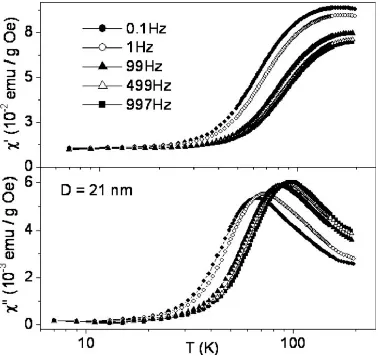
Figure 12. Experimental measurement results of a.c. susceptibility measurements of Ni nanoparticles dispersed in silica. Adapted from reference [57]. The average particle sizeD is shown as derived using transmission electron microscopy.

emitting a phonon of energy ∆ −δ to drop down to B. This is known as an Orbach process, which we have already described above. The relaxation rate of an Orbach process is proportional to the Bose factor (exp(∆/kBT)−1)−1 which is proportional to

exp(₋∆/kBT)if∆kBT (i.e. recovers the Arrenhius form in equation (57) withEa= ∆).

If the excited state C is virtual, it is known as a Raman process. The detailed functional form ascribed to these different relaxation processes can depend on the nature of the magnetic ion (Kramers or non-Kramers) and the temperature and field regime being studied. For example, a study of both a trigonal prismatic mononuclear Co(II) complex and mononuclear hexacoordinate Cu(II) complex found slow relaxation to be due to the sum of Orbach and quantum tunnelling processes, as well as direct and Raman phonon processes, and the data were fitted to an expression given by

τ−1_=AH2_T+ B1

1 +B2H2

+CTn_+τ−1

0 exp

−Ea kBT

,

1.0 10-5 1.5 10-5 2.0 10-5 2.5 10-5 3.0 10-5 3.5 10-5 4.0 10-5

(

m

3 mol -1 )

0.0 5.0 10-6 1.0 10-5 1.5 10-5

(

m

3 mol -1 )

2 3 4 5 6 7 8 9 10

Temperature (K)

2 3 4 5 6 7 8 9 10

Temperature (K)

10000 Hz 8000 Hz 6000 Hz 4000 Hz 2000 Hz

1500 Hz 539.1 Hz 193.7 Hz 69.6 Hz 25 Hz µ0Hd.c.= 0 T

(a)

(c) µ0Hd.c.= 0 T

µ0Hd.c.= 0.1 T

(b)

(d) µ0Hd.c.= 0.1 T

(e)

Figure 13.Results of a.c. susceptibility measurements on [CoIII

2 Er(L)2(µ-O2CCH3)2(H2O)3]·NO3·xMeOH·yH2O, known as Co2Er, in an ac

magnetic field ofµ0Hac= 0.4 mTadapted from reference [63]. (In the chemical formula, LH3=

2-methoxy-6-[2-(2-hydroxyethylamino)-ethyliminomethyl]phenol.) The (a) real and (b) imaginary parts of ac susceptibility in a d.c magnetic field ofµ0Hdc = 0 T. The (c) real

and (d) imaginary parts of ac susceptibility in a d.c magnetic field ofµ0Hdc= 0.1 T. (e) An ORTEP diagram of Co2Er from reference [63]

omitting disordered parts, H atoms, anions and solvent molecules for clarity .

0.0

2.5 10-6

5.0 10-6

7.5 10-6

1.0 10-5

1.25 10-5

1.5 10-5

(

m

3

mol

)

1.0 10-5 2.0 10-5 3.0 10-5 4.0 10-5

(

m

mol

)

2.0(1) K 2.6(1) K 3.0(1) K 3.4 K 3.6 K 4.0 K 4.6 K 5.0 K

Fit Fit Fit

µ0Hd.c.= 0.1 T

Figure 14.Cole-Cole plot of Co2Er measurements atµ0Hd.c c. = 0.1 Tshowing the formation of the expected arcs for a system displaying slow magnetic relaxation from reference [63]. Displayed fits to equation (48) are shown as lines.

of SMMs it is the Arrhenius type relaxation that is the relaxation of interest (in order to extract the height of the energy barrier,Ea). Thus a d.c field and frequency study must be performed to identify the conditions needed to minimise contributions to τ−1 _{from those} field-dependent parts [63, 67, 68].

These systems also provide a real example of the case of two τ’s (as described by equation (31)). The molecule (Cp∗_{)Er(COT) (where Cp}∗ _{is C}

5Me−5 and COT is C8H28−) features an Er(III) ion sandwiched between two carbon rings. Measurements of this compound revealed two separate sets of peaks appearing in χ00 _{at different ranges of temperatures}

[70]. A.c. data were successfully modelled via a version of equation (31) incorporating the generalised Debye model [70]. The source of two separate τ’s in this compound was suggested to be two separate conformations of (Cp∗_{)Er(COT) [70]. Similarly,}

J₁

J₂

J₃

J₄

J₅

J₆

Figure 15.A schematic of a typical spin glass. A low concentration of spins decorate a non-magnetic2-D square lattice. Due to their random locations the exchanges between each (Jifori = 1to6)

are also random leading to frustration.

4.3. Spin Glasses

A spin glass can be formed if one takes a non-magnetic lattice and populates it with a dilute random distribution of magnetic atoms, as shown in figure 15. An example is the CuMn system in which magnetic Mn atoms replace Cu atoms at the few per cent level [8]. Cu is a non-magnetic metal and so the exchange interactions between the Mn atoms are mediated through the conduction electrons by the RKKY interaction [21]

J(r)_∝cos(2kFr)

r3 , (60)

where _J is the exchange integral, kF is the Fermi wavevector and r is the distance between two Mn atoms. _J may be positve or negative (ferromagnetic or antiferromagnetic) depending on distance, thereby introducing frustration in the spin glasses (see figure 15). Spin glasses are therefore random, mixed-interacting systems which, when temperature is lowered, undergo a freezing transition from a paramagnetic state to a metastable state known as the glass or frozen state lacking in any long range magnetic order [8, 33, 71]. The glassiness arises from competing interactions between individual magnetic moments and leads to a multidegenerate ground state [8].

This multidegenerate ground state means that the system can adopt a number of equally favourable

orientations, but upon freezing the system becomes stuck in one particular configuration. Slow relaxations arise as individual magnetic moments begin to reorient, creating additional frustrations and further reorientation of other magnetic moments. This process is very complex because each magnetic moment occupies a different environment and so may be frustrated in a different way (due to the random site distribution and random exchange). As the freezing temperature, Tf, is approached from higher temperatures, some moments begin to cease behaving independently and start to form growing clusters [28]. A variety of size of clusters can coexist, leading to a wide distribution of relaxation times.

Early a.c. susceptibility measurements of spin glasses identified a distinctive cusp in the in-phase component, χ0, at Tf [8, 33, 71]. Interpreting a spin glass as a collection of superparamagnetic clusters can allow the use of equation (34) which explicitly incorporates a distribution of relaxation times in g(τ) [31], often assumed to be Gaussian [72] though this does not always hold [73]. In this interpretation, freezing occurs when a large proportion of the superparmagnetic clusters are below their respective TB. Sometimes data are fitted to equation (28) to crudely monitor the spread of relaxation times parameterized by α [8, 28]. This equates to assuming the distribution of relaxation times is given by equation (35) and is a sensible step in modelling should a spin glass indeed be comprised of superparamagnetic clusters (since superparamagnets with a symmetric distribution of sizes [56, 57] likely have a symnmetric distribution of relaxation times). All of these approaches gloss over the details of what is actually a complex interacting system (and is emphatically not a collection of Debye relaxors).

This problem of describing a spin glass as a collection of (non-interacting) superparamagnetic clusters can be examined by considering the nonlinear, third harmonic of the susceptibility. Both the alloy Cu97Co3 and spin glass Au96Fe4 show similar linear susceptibility cusps but differ in their real third harmonic [38]. It was found that this harmonic (expected as a negative divergence above and below the freezing temperature [37, 41]) could be modelled as a distribution of superparamagnetic particles for Cu97Co3but not for Au96Fe4suggesting that this could be used to differentiate the two behaviours [38]. This study did not vary frequency or a.c. amplitude so it is unclear what frequency dependence (if any) exists in these results.

Figure 16. Example a.c. susceptibility of spin glass (Eu0.2Sr0.8)S

atµ0Hd.c. = 0 Tandµ0Ha.c. = 0.01 mTfrom reference [74].

Filled shapes correspond toχ0 _{while empty refer toχ}00_{with◦ =} 10.9 Hz,= 261 Hzand4= 1969 Hz.

Figure 17.Cole-Cole plots of (Eu0.2Sr0.8)S atµ0Hd.c.= 0 Tand

µ0Ha.c. = 0.01 mTfrom reference [74]. Numbers in the plot

correspond to a.c. drive frequencies. Lines are a result of fits to the data assuming data to be symmetric.

broad distribution of relaxation times. In fact, the broader the distribution of relaxation times the broader and more rounded the expectedχ00_{peak. This}

peak occurs when the average relaxation time τavg matchesω−1_.

Since τavg is temperature dependent, the form of τavg(T) can be used to try to identify the type of relaxation. Although an Arrhenius expression can appear to be successful in modellingτ(T)(and would make physical sense if a spin glass were composed of identical superparamagnetic clusters), it invariably yields unphysical values of the parameters Ea andτ0 [8, 71, 74]. The interacting nature of spin glasses is better accounted for using the Vogel-Fulcher law

τ =τ0exp

_E

a kB(T−T0)

(61)

which is better suited to glass-like systems [71, 74, 75]. Here, Ea and τ0 remain the activation energy and characteristic relaxation time while T0 is a new parameter that accounts for the interactions occurring between moments in a spin glass [2, 76]. It should be noted that τ may be modelled by further equations [2, 77]. The frequency dependence of the extracted freezing temperature (the temperature at which χ0 _{takes its maximum) is given by f =} d lnTf/d lnω. (Of course one can equivalently write f = d log10T /d log10ω.) In experiments Tf changes by a small amount asωchanges over several orders of magnitude, and sof can be estimated using

f = ∆Tf

Tf∆[ln(ω)]

. (62)

Iff is a constant thenTf ∝ωf. Spin glasses typically give a value off between0.001and0.08(much larger values are found for single molecule magnets [1, 8]) and thusTfhas a very weak frequency dependence.

While the discussion of this section has been concerned with the spin glass state emerging out of the paramagnetic state as temperature is lowered, spin glass-like states (with associated slow magnetic relaxation) have been studied emerging in other scenarios. The reentrant spin glass is one such example where a spin glass-like freezing occurs below a ferromagnetic transition [33, 78, 79] though it has been suggested this is not a true spin glass state [80]. The d.c. magnetisation increases as temperature is lowered due to the appearance of the ferromagnetic state, but decreases at even lower temperatures due to freezing [80, 81]. Figure 18 shows the χ00 _{peaks associated with the reentrant spin glass}

Figure 18. Imaginary part of the a,c, susceptibility of La0.8Sr0.2Mn0.925Ti0.075O3 demonstrating a reentrant spin glass.

The peaks at∼170 Kcorrespond a ferromagnetic transition while the lower set are associated with the slow relaxation of the frozen state. The inset highlights these peaks. Adapted from reference [81].

displays spin glass-like slow magnetic relaxation that persists in the presence of the superconductivity in the iron selenide layers [83].

4.4. Spin Ice

As with spin glasses, spin ices show slow magnetic dynamics. However, while intrinsic randomness is important in explaining these dynamics in spin glasses, a different explanation is needed for spin ices which have a completely ordered chemical composition. Spin ice behaviour was first identified in certain rare-earth pyrochlores [84]. Pyrochlores have formula A2B2O7 and contain a rare earth A which resides on the vertices of a network of corner-sharing tetrahedra [84, 85]. When A = Dy or Ho and B = Ti, the crystal field associated with the A cations exhibits strong Ising anisotropy that causes each A spins to lie along the line joining the centres of the two neighbouring tetrahedra which share the corner occupied by the A cation (these lines are along the _h111_i directions). Each spin can lie parallel or antiparallel to this line. The dipolar interaction and weak antiferromagnetic superexchange results in an effective ferromagnetic interaction. This, in combination with the single-site anisotropy, results in a spin arrangement that is subject to a constraint on each tetrahedron such that its four spins, one on each corner, should satisfy P

iS~i = 0. Thus two of the spins point into the centre of each tetrahedron while the other two point out, akin to the proton rules of water ice [86, 87]. There are a large number of ways of satisfying this constraint and so this results in a degenerate ground-state configuration (lacking long-range order down to low temperatures) [84, 88].

A.c. magnetic susceptibility measurements on spin ice show an Arrhenius-like behaviour at high

temperature (due to single ion processes and mixing with excited states) but on cooling the dynamics begin to freeze out [89]. This behaviour can look superficially like that of spin glasses, with a low temperature peak in d.c. susceptibility accompanied by a divergence between ZFC and FC sweeps. This is expected as in both cases a slowing down of spin dynamics is occurring.

The low-temperature excitations of spin ice have attracted considerable attention. A single spin-flip breaks the 2-in, 2-out constraint if the spin ice, creating a “three in/one out” and “three out/one in” pair of tetrahedra. This state can be considered as a monopole-antimonopole pair [88, 90] and further spin flips allow the monopole and antimonopole to separate, travelling through the lattice (the initial spin flip is said to have been “fractionalised”). Slow magnetic dynamics in the low-temperature state of a spin ice system can therefore be described by considering monopole motion. In fact, an early description of spin ice magnetic relaxation by Ryzhkin [88] was formulated by exploiting the analogy with dielectric relaxation in water ice. In this approach, the magnetic monopole current densityJ =

∂M/∂tcan be written as

J =κ(H₋χ−T1M), (63)

where κ is the monopole conductivity [88, 91]. In equilibrium, M = χTH and J = 0. Out of equilibrium, the monopole current contains two terms, the familiar drift term and the more unusual reaction field (originating from configurational entropy of the monopole vacuum i.e. the statistical mechanics of the spin configurations subject to topological constraints), and these two terms will not cancel. To understand the time dependence, it is helpful to Fourier transform equation (63) which results in

˜

J =₋iωM˜ =κ( ˜H₋χ−1

T M˜) (64)

and hence the magnetic susceptibility χ(ω) = ˜M /H˜ can be written as

χ(ω) = χT

1−iωτ, (65)

where τ = χT/κ; this is clearly Debye-like. We note that this approach can be extended to spatial deviations, resulting in a diffusion term being added to equation (63) as follows:

J(r) =κ[H(r)−χ−T1M(r)] +D∇

2_M

(r). (66)

Another approach [92] is to include a phenomenolog-ical inertial term into equation (63) to model a relax-ation of the monopole current and this leads to

χ(ω) = χT

Figure 19. Results of low temperature a.c. susceptibility measurements on spin ice Dy2Ti2O7 from reference [93] at

µ0Hd.c.= 0 Tandµ0Ha.c.= 0.5 mT.

where γ is a monopole current relaxation rate. This equation (which is equivalent to equation (18)) has been used to model data obtained in the quantum spin ice Yb2Ti2O7[18].

We now consider the specific example of Dy2Ti2O7, which is one of the most highly studied ex-amples of a classical spin ice. The low temperature (_∼ 1 K) peak in χ0 _{shown in figure 19 matches the}

freezing transition appearing in the d.c. susceptibil-ity. However, a.c. susceptibility reveals a peak inχ00_at

higher temperature (up to_∼ 20K) measured at high ω [93, 89] (not shown here). The arcs in the Cole-Cole plots in figure 20 allow these data to be mod-elled and the average relaxation timeτ(T)can be ex-tracted, as shown in figure 21. The clearly asymmetric arcs were modelled with the Cole-Davidson model fea-turing a maximum cut-off relaxation time and a long low-τ tail [93]. The origin of this behaviour was un-clear beyond being related to the spin ice state [93]. The relaxation time increases on cooling in the ther-mally activated high-temperature regime (associated with excitations to higher crystal field levels), enter-ing a plateau region below around 12 K (associated with quantum tunnelling processes through the crystal field barrier), before experiencing a sharp upturn be-low around 2 K (associated with monopole dynamics), explainable only by including the Coulomb interaction between charges [94].

4.5. Long Range Magnetic Order

Our discussion so far has focused on systems lacking long range order. However, slow magnetic relaxation can also be observed in systems with long range order

Figure 20.Cole-Cole plot of frequency dependent feature of Results of Dy2Ti2O7 from reference [93]. µ0Ha.c. = 0.5 mTandχ0_int

andχ00_intindicateχ0andχ00corrected for the demagnetizing factor. Panel (b) is a blow-up of panel (a), while panel (c) shows high temperature fits to the Cole-Davidson model (equation (29)).

if they contain some component which responds rather sluggishly. The pertinent question is: “What is the sluggish entity?” Consider first a ferromagnet in which each spin is coupled to a neighbour by an exchange constant J. The dynamics of the spins occurs on a frequency scale given by J/~ which is always far in excess of anything detectable by a.c. susceptibility (and hence spin waves are studied using neutron scattering, see figure 2). However, the simple, fully-aligned ferromagnetic state is not usually obtained during a ZFC susceptibility measurement because the sample breaks up into domains.