INFORMS is located in Maryland, USA
Management Science
Publication details, including instructions for authors and subscription information: http://pubsonline.informs.org
Time Matters Less When Outcomes Differ: Unimodal vs.
Cross-Modal Comparisons in Intertemporal Choice
Robin Cubitt, Rebecca McDonald, Daniel Read
To cite this article:
Robin Cubitt, Rebecca McDonald, Daniel Read (2018) Time Matters Less When Outcomes Differ: Unimodal vs. Cross-Modal Comparisons in Intertemporal Choice. Management Science 64(2):873-887. https://doi.org/10.1287/mnsc.2016.2613
Full terms and conditions of use: http://pubsonline.informs.org/page/terms-and-conditions
This article may be used only for the purposes of research, teaching, and/or private study. Commercial use or systematic downloading (by robots or other automatic processes) is prohibited without explicit Publisher approval, unless otherwise noted. For more information, contact [email protected].
The Publisher does not warrant or guarantee the article’s accuracy, completeness, merchantability, fitness for a particular purpose, or non-infringement. Descriptions of, or references to, products or publications, or inclusion of an advertisement in this article, neither constitutes nor implies a guarantee, endorsement, or support of claims made of that product, publication, or service.
Copyright © 2017, The Author(s)
Please scroll down for article—it is on subsequent pages
INFORMS is the largest professional society in the world for professionals in the fields of operations research, management science, and analytics.
http://pubsonline.informs.org/journal/mnsc/ ISSN 0025-1909 (print), ISSN 1526-5501 (online)
Time Matters Less When Outcomes Differ: Unimodal vs.
Cross-Modal Comparisons in Intertemporal Choice
Robin Cubitt,aRebecca McDonald,bDaniel Readb
aSchool of Economics and Centre for Decision Research and Experimental Economics, University of Nottingham, Nottingham NG7 2RD,
United Kingdom; bWarwick Business School, University of Warwick, Coventry CV4 7AL, United Kingdom Contact: [email protected](RC); [email protected](RM); [email protected](DR)
Received:March 5, 2015 Revised:April 5, 2016 Accepted:April 27, 2016
Published Online in Articles in Advance: February 16, 2017
https://doi.org/10.1287/mnsc.2016.2613
Copyright:© 2017 The Author(s)
Abstract. Unimodal intertemporal decisions involve comparing options of the same type (e.g., apples now versus apples later), and cross-modal decisions involve comparing options of different types (e.g., a car now versus a vacation later). As we show, exist-ing models of intertemporal choice do not allow time preference to depend on whether the comparisons to be made are unimodal or cross-modal. We test this restriction in an experiment using thedelayed compensation method, a new extension of the standard method
of eliciting intertemporal preferences that allows for assessment of time preference for nonmonetary and discrete outcomes, as well as for both cross-modal and unimodal com-parisons. Participants were much more averse to delay for unimodal than cross-modal decisions. We provide two potential explanations for this effect: one drawing on multiat-tribute choice, the other drawing on construal-level theory.
History:Accepted by Yuval Rottenstreich, judgment and decision making.
Open Access Statement:This work is licensed under a Creative Commons Attribution 4.0 International License. You are free to copy, distribute, transmit and adapt this work, but you must attribute this work as “Management Science. Copyright ©2017 The Author(s). https://doi.org/10.1287/ mnsc.2016.2613, used under a Creative Commons Attribution License:http://creativecommons .org/licenses/by/4.0/.”
Funding:The authors are grateful for assistance from the Economic and Social Research Council [Grant ES/K002201/1] and the Leverhulme Trust [Grant RP2012-V-022].
Supplemental Material:Data are available athttps://doi.org/10.1287/mnsc.2016.2613.
Keywords: intertemporal choice • decision modelling • economics: behavior and behavioral decision making • delay discounting
Introduction
In intertemporal choices, the objects of choice are dis-tributed over time, so decision makers face variations not only in what the outcomes are but also in when they are received. Examples include whether to go to a movie tonight or a football game tomorrow, whether to take a job in sales now or to graduate and then seek a professional career, or whether to buy a car now or wait five years and build an extension to the house.
Conflicts between the “what” and the “when” are central to empirical and theoretical accounts of time preference (for surveys, see Frederick et al.
2002, Manzini and Mariotti 2009, and Urminsky and Zauberman 2014). Such accounts usually focus on trade-offs betweenquantityandtiming. In much of the empirical literature, the options are different quanti-ties of money at different dates (e.g., $100 now versus $120 in 12 months). When the options are not sums of money, they are generally different quantities at differ-ent dates of some nonmonetary object or commodity (e.g., chocolates, the number of lives saved, grams of cocaine).1
However, many real-world choices (including the examples in our opening paragraph) do not reduce to
a trade-off between timing and the quantity of a given good. Instead, not only do the goods differ in when they occur, but also in what they are. We call such choicescross-modal. These can be contrasted with uni-modal choices, where the options are the same good at different dates, even if perhaps in different quanti-ties. We will focus on the relationship between con-siderations of timing and concon-siderations of what the object to be received is by setting variations in the quantity of goods to one side and concentrating on choices between single items at different dates. Obvi-ously, such choices may still be cross-modal or uni-modal. For example, to introduce some cases from the experiment reported below, the choice between a box of chocolates today and a fountain pen in 60 days is cross-modal, whereas that between a fountain pen today and an identical pen in 60 days is unimodal. We investi-gate whether time preference operates in the same way (and to the same degree) in cross-modal and unimodal choices. Our motivation for this is twofold.
First, as just noted, many everyday intertemporal decisions are cross-modal, whereas empirical research on time preference has usually followed a unimodal 873
paradigm. Although people do face unimodal deci-sions in their personal finances, it remains a largely neglected question how far the lessons of unimodal research extend to those everyday decisions that are cross-modal.2
Second, the issue of whether time preference operates differently in cross-modal compared with unimodal choices marks a divide between two approaches to modelling: one value-based, the other attribute-based. The former rests on a classic view that intertempo-ral choices reduce to comparisons of values (typically, discounted present values), with each option having a value independent of its alternatives. On this account, it should make no fundamental difference whether the decisions through which time preference is revealed are cross-modal or unimodal. We present an experimen-tal test of this prediction, taking as our starting point a baseline value-based model of the strength of time preference. As we will make precise below, this model predicts that overall aversion to delay is the same for cross-modal and unimodal decisions.
If this prediction were confirmed, it would be good news for those who seek to generalise findings from research on unimodal decisions. But we find instead that our participants are considerably more patient in the cross-modal than in the unimodal choices that we pose to them. Although this finding contradicts our baseline model, it is consistent with earlier research showing that the standard (unimodal) way of elicit-ing time preferences appears to exaggerate observed impatience relative to other elicitation procedures (e.g., Frederick2003; Read et al.2005,2013). More important, greater patience in cross-modal discounting chimes well with an attribute-based approach. The finding is quite intuitive if the weight that a difference in tim-ing carries in participants’ intertemporal decision mak-ing depends on how many other differences between options there are to consider. We sketch an account of our findings in this form, as well as a further account that suggests the mental representations of options dif-fer in unimodal and cross-modal choice.
To investigate whether revealed aversion to delay differs systematically in strength between cross-modal and unimodal decisions, we develop a way to measure it that can be applied regardless of whether the options differ in ways other than timing and quantity. This is thedelayed compensation method.
The Delayed Compensation Method
In the delayed compensation method (henceforth, DCM), a participant first chooses between two options that each specify a good to be received and a date of receipt. The options may differ in the good, the date, or both. As in the example introduced earlier, the options might be a box of chocolates today and a pen in 60 days, or they might be a pen today and an identi-cal pen in 60 days. The decision maker indicates which
option she prefers and the delayed monetary compen-sation she requires to make her just willing to accept the dispreferred option instead of the preferred one. Regardless of the direction of the initial preference, monetary compensation is paid in a common period that comes after the later of the two options’ delivery dates (hence “delayed” compensation).
The DCM has several noteworthy features. First, by capturing preference trade-offs using monetary com-pensation, we avoid the need for divisibility in goods. By paying that compensation at a common date (for all tasks), we avoid the need for auxiliary assump-tions about the discounting of money. By having the common compensation date after the date of receipt of the later good, we ensure the compensation cannot be used to purchase either option. By using compen-sation for having a dispreferred option instead of a preferred one (regardless of which would be received earlier), we guarantee that the compensation is posi-tive and so avoid any need to take money from partic-ipants and any suggestion that they “ought” to prefer earlier options. We also avoid any confound with loss aversion, such as might be introduced if we sometimes elicited willingness to accept and sometimes willing-ness to pay, or if we gave participants one of the options as an initial endowment. Finally, as this paper’s imple-mentation of it shows, the DCM allows strength of time preference to be assessed without varying quantities of consumption goods, thereby preventing any resulting confounds with diminishing marginal utility.
The Fisher Diagram
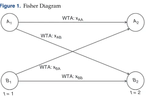
Figure 1 provides a representation of the DCM and allows us to refine the question of whether time prefer-ence differs between cross-modal and unimodal com-parisons. We call the figure the Fisher diagram, as it is inspired by Chart 4 from Irving Fisher’s Theory of Interest(1930).
Figure1 shows two goods (Aand B) and two time periods (t1,2) in which a good might be received.
Together, these ingredients define four options, or dated goods (A1,A2,B1,B2), shown in circles. (As explained below, we letAbe the good that is preferred when timing is not an issue. So using our earlier exam-ples and for someone who prefers chocolates to a pen, A1 could be a box of chocolates today andB2a pen in 60 days.)
In the Fisher diagram, the two horizontal arrows rep-resent unimodal intertemporal comparisons; the two diagonal arrows, cross-modal ones. In our unimodal comparisons, the options differ only in the timing of receipt; in cross-modal comparisons, the options differ in the good to be received as well as the timing.3
In the DCM, the agent is faced with a choice at (or before) period t1 between two options, which are
dated goods from Figure1. She will receive one of the
Figure 1.Fisher Diagram
A1 A2
B1 B2
WTA: xAA
WTA: xAB
WTA: xBA
WTA: xBB
t = 1 t = 2
Notes. The Fisher diagram shows the different goods (AandB) at specified times (t1 andt2) and the four different comparisons
between goods at different dates. For each pair of dated goods, the WTA is the monetary amount that, when given in addition to the dispreferred of the two options, will make the agent just willing to take the dispreferred instead of the preferred option. The figure shows a case where, in all four intertemporal comparisons, thet1
option is preferred.
options at the time specified. She is required to state the monetary compensation to be received at period t3 (i.e., some fixed time after periodt2) that is just
sufficient to make her willing to accept her dispreferred option instead of her preferred one. In the language of economics, this is her willingness to accept (WTA).
The only assumption on preferences that the DCM requires is that the agent has preferences over the dated goods and can specify the relevant compensations. To streamline the exposition, we set out some additional default assumptions imposed unless otherwise stated: the agent prefers receiving any of the dated goods of Figure1to receiving nothing and has strict preferences between them.4 There is one good—we name it A— that the agent prefers to the other good whenever both would be delivered in the same period (i.e.,A1is pre-ferred to B1, and A2 is preferred to B2).5 The agent prefers any good delivered at t1 to the same good
delivered at t2 (i.e., A1 is preferred to A2, and B1
is preferred to B2). Given transitivity, it then follows thatA1is preferred, andB2dispreferred, to every other option. The intuition is thatA1is the better good, with the added advantage of early delivery, whereasB2 is the worse good, with the added disadvantage of late delivery. These default assumptions do not determine preference betweenB1andA2. AsB1is the worse good but sooner, whereasA2 is the better good but later, it is possible to preferB1toA2orA2toB1. Our analysis will cover both cases.
We start with an agent who prefers B1 to A2 and therefore prefers the earlier option in any given pair. For her, the DCM always elicits the monetary compen-sation just sufficient to induce acceptance of the later option instead of the earlier. We usexAA to denote the compensation required to acceptA2instead ofA1,xBB
denotes the compensation required to acceptB2instead ofB1,xABdenotes the compensation required to accept B2 instead of A1, and xBA denotes the compensation required to acceptA2instead ofB1. The first subscript indicates the good in the earlier and preferred option; the second subscript, the good in the later and dispre-ferred option. So xAB and xBA relate to different com-parisons, as Figure1makes clear.
The next section sets out a baseline value-based model from which we derive precise predictions, but we end this section by giving a parallel intuitive argu-ment. When B1 is preferred to A2 and the default assumptions hold, the agent prefersA1toB1toA2toB2. So, from a value-based perspective, we would expect the cross-modal compensation term xAB to be the largest of the four,xBA the smallest, and the unimodal terms intermediate. Intuitively, xAB is large because it includes compensation not only for delay but alsofor taking the worse good (B) rather than the better one (A), andxBAis small because the disadvantage of delay is partlyoffsetby taking the better good (A) rather than the worse one (B). AsxAB andxBA are driven in oppo-site directions by the difference between the better and worse goods, we compare their sum [xAB+xBA] to the corresponding sum [xAA+xBB] of unimodal compen-sations. If the difference between goodAand goodB has equal and opposite impacts onxAB andxBA, those impacts will cancel in the cross-modal sum, leaving only the influences of delay. These influences will be the same as those that drive the unimodal sum if (as a value-based perspective implies) there is no funda-mental difference between attitude to delay in cross-modal and unicross-modal comparisons. This leads to the prediction that, whenB1is preferred toA2, [xAB+xBA] will equal [xAA+xBB]. This prediction is made formally in the next section, which also provides a correspond-ing prediction for whenA2is preferred toB1.
A Baseline Model
We now present a model of the preferences the agent has at the point of decision in the DCM (at or before t1) and how they determine the four WTA
com-pensation terms. This model is premised on maximiza-tion of decision utility and encompasses all commonly cited discounting frameworks (including exponential, hyperbolic, quasi-hyperbolic, and constant sensitivity forms). We specify that decision utility depends on dated goods to be received and delayed monetary compensation, and it is additively separable in those two sources of utility. Although the DCM is a general framework, as we apply it in this paper, the agent is restricted to receive one unit of one dated good, so we define a distinct utility for the receipt of each of these goods, usinga1,a2,b1, andb2as the utility terms forA1, A2, B1, and B2, respectively. These terms reflect both the nature of the good to be received and any delay
until that occurs.6Finally, we definev( · )as an increas-ing function of monetary compensation att3 and set
v(0)0.7 We refer to v( · )as utility of money. Unless
otherwise stated, we assume that it is linear in delayed compensation. AppendixAcovers the case of dimin-ishing marginal utility of money and gives more detail on other aspects of the model.
We begin with an agent who prefers B1 to A2, as in the previous section. The unimodal WTAsxAA,xBB and the cross-modal WTAsxAB,xBA (see Figure1) are defined by the following equations:
a1a2+v(xAA), (1.i) b1b2+v(xBB), (1.ii) a1b2+v(xAB), (1.iii) b1a2+v(xBA). (1.iv) In each case, the left-hand side is the utility of the pre-ferred option, the first term on the right-hand side is the utility of the dispreferred option, and the final term that of the compensation required to accept the dispre-ferred option. It follows by simple arithmetic that
v(xAA)+v(xBB)(a1−a2)+(b1−b2)
(a1−b2)+(b1−a2)
v(xAB)+v(xBA). (2)
Withv( · )linear, this implies that
xAA+xBBxAB+xBA. (3) Equation (3) is the prediction stated in the previous section for an agent who prefersB1toA2.
Figure1provides the key intuitions of our baseline model. First, look atxAB and xAA. Each is a compen-sation for forgoing the earlyA1in exchange for a later option: forB2inxABand forA2inxAA. SinceB2is worse than A2,xAB exceeds xAA; it does so by an amount determined by the difference in utility between the two delayed goods and by the utility function for money, v( · ). Now, look at xBB and xBA. As Figure 1 shows, each is a compensation for forgoing B1: forB2 in xBB and forA2inxBA. As the agent thinksB2is worse than A2,xBB exceeds xBA by an amount again determined by the utility difference between the delayed goods and by v( · ). So, for any given v( · ), the difference in utility betweenA2andB2determines both [xAB−xAA] and [xBB−xBA]. Withv( · )linear,xAB−xAAxBB−xBA, which rearranges to give Equation (3).
As an example using our experimental goods, imag-ine Alice prefers the chocolates to the pen (so, for her, good Achocolates) and that her function v( · ) has
the simplest linear formv(x)x, so the compensation
terms are given directly by differences in the decision utilities of dated goods. Let those utilities be 30 and 25, respectively, for the chocolates and pen at t 1; let
the utilities be 24 and 20, respectively, for the choco-lates and pen at t2. In the unimodal comparisons,
Alice demands compensations of 6 (30−24) for
delay-ing the chocolates and 5 (25−20) for delaying the
pen. In the cross-modal comparisons, she demands 10 (30−20) for taking the delayed pen instead of early
chocolates and 1 (25−24) for taking delayed
choco-lates instead of the early pen. The cross-modal com-pensations have the same sum as the unimodal ones: 10+16+5. Equivalently, and reflecting the argument
of the previous paragraph, 10−65−14; 4 is the
dif-ference in utility between the delayed chocolates and the delayed pen.
We now adapt the analysis for an agent who prefers A2 toB1. The terms xAA, xBB, and xAB are defined as before by Equations (1.i)–(1.iii). However, compensa-tion in the DCM always accompanies the least pre-ferred good. Therefore,xBAis undefined for this agent, and compensation to achieve indifference between those two options must now accompany the dispre-ferred B1. We use yBA to denote this compensation, which is governed by
a2b1+v(yBA). (1.iv’) By simple arithmetic, using (1.i)–(1.iii) and (1.iv’),
v(xAA)+v(xBB)(a1−a2)+(b1−b2)
(a1−b2) − (a2−b1)
v(xAB) −v(yBA). (2’)
With v( · )linear, this implies that, for an agent who prefersA2toB1,
xAA+xBBxAB−yBA. (3’) The only difference between (3’) and (3) is that−yBA appears in place of+xBA.8
To contrast −yBA with +xBA, consider the case of Bob who, like Alice, prefers the chocolates to the pen (so again, goodAchocolates) and hasv(x)x. But
Bob very strongly prefers the chocolates. For him, the utilities are 50 and 25, respectively, for the chocolates and pen at t1 and 40 and 20, respectively, for the
chocolates and pen att2. In the unimodal
compar-isons, Bob demands compensations of 10 (50−40)
for delaying the chocolates and 5 (25−20) for
delay-ing the pen. In the cross-modal comparisons, however, he demands 30 (50−20) for taking the delayed pen
instead of early chocolates. But Bob likes chocolates enough to take the delayed chocolates over the earlier pen and demands 15 (40−25) for taking the earlier
pen instead. The compensation of 15 is yBA, and the equality in Equation (3’) holds: 10+530−15.
We place both+xBA and−yBA and their equivalents
for other pairs under the umbrella termcost of delay. For any pair of dated goods with different delivery dates,
this is the compensation required to accept the later good when the earlier is preferred—and the negative of the compensation required to accept the earlier good when the later is preferred. Thus, while compensation for taking a dispreferred option is always positive, cost of delay can be negative. Our null hypothesis, based on the baseline model of behaviour in the setup of Fig-ure1, can then be stated in the general form: the sum of the two unimodal costs of delay equals the sum of the two cross-modal costs of delay.9
As we have shown, this hypothesis is robust to whether the agent prefers the “better but later” good (A2) to the “worse but earlier” good (B1), or vice versa. However, it does depend on the function v( · ) being linear. Arguably, linearity of utility in money is a suit-able assumption for the relatively small sums needed to compensate for differences between the goods used in the experiment. However, concavity of v( · ) is an obvious alternative specification, which, as we show in AppendixA, does matter: withv( · )concave, the model predicts the sum of costs of delay will be greater for cross-modal comparisons than for unimodal ones.
The restrictions we derive from our baseline model are not specific to the traditional Samuelsonian dis-counted utility model (Samuelson 1937) but apply equally to a whole family of models from economics and psychology. The model makes no assumptions about whether there is a single discount function, separate discounting for goods and money, and/or good-specific discount functions.10 The gaps between periodst1,2, and 3 can be of any calendar duration;
given their durations, any decreasing discount func-tion is allowed.
Experiment
We have conducted a series of studies comparing uni-modal and cross-uni-modal intertemporal choices, using variations of the DCM. Here, we present only the “flag-ship” study. Its results are representative of all of the studies.11
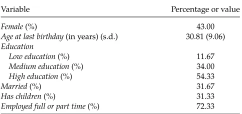
The study was programmed in Qualtrics and con-ducted online in August 2014 using the Amazon Mechanical Turk online labour market. After the tasks described below, participants answered follow-up questions and provided basic demographic infor-mation, summarised in Table1.
Design and Method
[image:6.612.314.556.88.202.2]The design was an implementation of the DCM. The goods were a good-quality fountain pen by Lamy and a box of 36 luxury chocolates by Godiva. They were selected because they could be sourced from Ama-zon.com, and because their prices were similar (about $30 each on Amazon at the time). We ordered the items for participants either “today” or “in 60 days” as appropriate, to be delivered (free) to the participant’s
Table 1. Demographics(n300)
Variable Percentage or value
Female(%) 43.00
Age at last birthday(in years) (s.d.) 30.81 (9.06)
Education
Low education(%) 11.67
Medium education(%) 34.00
High education(%) 54.33
Married(%) 31.67
Has children(%) 31.33
Employed full or part time(%) 72.33
Notes. Low educationis defined not having begun university.Medium educationis being currently at university.High educationis having completed university.
address. Thus, the four dated goods were a pen today, a pen in 60 days, a box of chocolates today, and a box of chocolates in 60 days. The experiment elicited the com-pensation needed to induce the participant to accept the dispreferred one out of a pair of options, each of which was one of these dated goods. Compensation was in the form of Amazon.com gift certificates, deliv-ered in 90 days, which could be used by the participant effectively as money at that time.
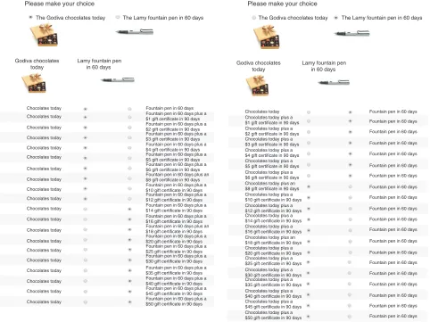
There were four choice conditions: two based on uni-modal choices (chocolates today or in 60 days; a pen today or in 60 days) and two based on cross-modal choices (chocolates today or a pen in 60 days; a pen today or chocolates in 60 days). Each participant was assigned to one condition. Before starting the task, participants were shown pictures and brief descrip-tions of the goods. They then made a single choice between the options. Depending on what they chose, they were then assigned to a choice list following the logic depicted in Figures2(a) and2(b). The first row in the choice list repeated the initial choice, and in subse-quent rows, the dispreferred option was supplemented with compensating money amounts to be delivered in 90 days. The second row combined compensation of $1 in 90 days with the item they did not originally choose. This compensation increased down the choice list in $1 increments to $6, then in $2 increments to $20, and $5 increments up to a maximum of $50. We chose this maximum because it comfortably exceeded the Ama-zon.com price of each item.
The decisions of two hypothetical individuals are illustrated in Figure 2. For the purposes of analysis, we measure the indifference point as the midpoint between the highest amount that would not induce the participant to switch and the lowest amount that would. So in Figure2(a), compensation for taking the pen later over the chocolates is $13, or the midpoint between the $12 turned down and the $14 accepted. The individual in Figure 2(b) prefers the pen later over the chocolates today and requires an estimated $7
Figure 2.(Color online) Example Choice Lists
(a) Initial preference for the chocolates today
Please make your choice
The Godiva chocolates today The Lamy fountain pen in 60 days
(b) Initial preference for the pen in 60 days
Please make your choice
The Godiva chocolates today The Lamy fountain pen in 60 days
Godiva chocolates
today Godiva chocolatestoday
Lamy fountain pen
in 60 days Lamy fountain penin 60 days
Chocolates today
Chocolates today Chocolates today plus a $1 gift certificate in 90 days Chocolates today plus a $2 gift certificate in 90 days Chocolates today plus a $3 gift certificate in 90 days Chocolates today plus a $4 gift certificate in 90 days Chocolates today plus a $5 gift certificate in 90 days Chocolates today plus a $6 gift certificate in 90 days Chocolates today plus an $8 gift certificate in 90 days Chocolates today plus a $10 gift certificate in 90 days Chocolates today plus a $12 gift certificate in 90 days Chocolates today plus a $14 gift certificate in 90 days Chocolates today plus a $16 gift certificate in 90 days Chocolates today plus an $18 gift certificate in 90 days Chocolates today plus a $20 gift certificate in 90 days Chocolates today plus a $25 gift certificate in 90 days Chocolates today plus a $30 gift certificate in 90 days Chocolates today plus a $35 gift certificate in 90 days Chocolates today plus a $40 gift certificate in 90 days Chocolates today plus a $45 gift certificate in 90 days Chocolates today plus a $50 gift certificate in 90 days Chocolates today Chocolates today Chocolates today Chocolates today Chocolates today Chocolates today Chocolates today Chocolates today Chocolates today Chocolates today Chocolates today Chocolates today Chocolates today Chocolates today Chocolates today Chocolates today Chocolates today Chocolates today Chocolates today
Fountain pen in 60 days Fountain pen in 60 days plus a $1 gift certificate in 90 days Fountain pen in 60 days plus a $2 gift certificate in 90 days Fountain pen in 60 days plus a $3 gift certificate in 90 days Fountain pen in 60 days plus a $4 gift certificate in 90 days Fountain pen in 60 days plus a $5 gift certificate in 90 days Fountain pen in 60 days plus a $6 gift certificate in 90 days Fountain pen in 60 days plus an $8 gift certificate in 90 days Fountain pen in 60 days plus a $10 gift certificate in 90 days Fountain pen in 60 days plus a $12 gift certificate in 90 days Fountain pen in 60 days plus a $14 gift certificate in 90 days Fountain pen in 60 days plus a $16 gift certificate in 90 days Fountain pen in 60 days plus an $18 gift certificate in 90 days Fountain pen in 60 days plus a $20 gift certificate in 90 days Fountain pen in 60 days plus a $25 gift certificate in 90 days Fountain pen in 60 days plus a $30 gift certificate in 90 days Fountain pen in 60 days plus a $35 gift certificate in 90 days Fountain pen in 60 days plus a $40 gift certificate in 90 days Fountain pen in 60 days plus a $45 gift certificate in 90 days Fountain pen in 60 days plus a $50 gift certificate in 90 days
Fountain pen in 60 days Fountain pen in 60 days
Fountain pen in 60 days
Fountain pen in 60 days
Fountain pen in 60 days Fountain pen in 60 days
Fountain pen in 60 days Fountain pen in 60 days
Fountain pen in 60 days
Fountain pen in 60 days
Fountain pen in 60 days Fountain pen in 60 days
Fountain pen in 60 days
Fountain pen in 60 days
Fountain pen in 60 days
Fountain pen in 60 days Fountain pen in 60 days Fountain pen in 60 days Fountain pen in 60 days Fountain pen in 60 days
Notes. The figure shows how either initial choice (between chocolates today and a pen in 60 days) would be followed by a choice list in which participants would indicate their WTA to take the option they did not initially choose instead of their initially preferred option. Each participant would see the choices from either (a) or (b).
(midpoint between $6 and $8) to take the chocolates today.12
To test for convergent validity of our unimodal measures, we elicited two conventional measures of time discounting after participants had completed the DCM. One measure consisted of choices between smaller–sooner and larger–later amounts of money, selected from Kirby et al. (1999). The other was a matching task adapted from Van den Bergh et al. (2008). The participants stated the delayed sum they regarded as just as good as $15 now, where the delays were one week and one month, and time preference was measured using the area-under-the-curve method (Myerson et al.2001). Since these tasks are unimodal, we should expect responses to them to correlate with those to the unimodal tasks of the DCM.
In total, 324 U.S. residents completed the survey. We excluded 24 who had opted out of receipt of goods, and hence the incentivisation, by not providing an email
address.13 Every participant was given a five-digit ID number. We randomly selected 37 of these numbers to identify participants to receive one of their choices for real, i.e., the option they had chosen in one initial choice or one row of a choice list. This choice would either be a good or a good plus monetary compensa-tion in the form of an Amazon.com gift voucher. All participants were informed that one in nine of them would receive a choice for real and that the list of all chosen ID numbers would be emailed to everybody, followed by emails to the chosen participants indicat-ing what they would receive and when. The gift vouch-ers sent out as monetary compensation were worth $20.21 on average.
Results
Initial Choices. We first consider the initial choices be-tween goods unaccompanied by monetary compensa-tion. For unimodal choices, the great majority chose
the earlier option: 84% (65/77) for chocolates and 84% (62/74) for the pen. For cross-modal choices, the pro-portion choosing the earlier option was much lower: 61% (48/79) chose chocolates now over a pen later, and 51% (36/70) chose a pen now over chocolates later. Because these proportions are lower (p <0.001) for
cross-modal than unimodal, cross-modal choices are at least partly determined by preferences over goods. Because they sum to more than 100% (albeit not sig-nificantly;p0.124), choices also seem at least partly
determined by time. Time, however, is not decisive, since 43% (65/149) of participants facing a cross-modal choice chose the delayed option.
Cost of Delay. Our main question is whether the im-pact of time is the same when making cross-modal and unimodal choices. This is measured by cost of delay.
The baseline model predicts that, for each individ-ual, the sum (or, equivalently, the average) of that indi-vidual’s two cross-modal costs of delay equals the sum (respectively, average) of their two unimodal costs of delay. In our design, each participant reveals the cost of delay for one pair of options. Random assignment to groups then implies that, if the baseline model is correct, we should find the average cost of delay across the participants completing cross-modal tasks equal to average cost of delay across the participants com-pleting unimodal cases. But that is not at all what we observe.
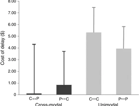
Figure 3 shows the cost of delay for each pair of options, averaged across participants making the choice between those options. Each cross-modal col-umn in the figure is markedly shorter than each uni-modal column, indicating that average observed cost of delay is lower for cross-modal than unimodal com-parisons. More precisely, the mean values for cost of delay in each of the comparisons are as follows:
Unimodal—chocolates: cost of delay$5.31,
Unimodal—pens: cost of delay$3.91,
Chocolates now, pens later: cost of delay$0.12,
Pens now, chocolates later: cost of delay$0.86.
Aggregating across chocolates and pens, the mean cost of delay is much lower for cross-modal compar-isons ($0.46) than for unimodal ones ($4.63), and the difference is statistically significant (p0.006).
[image:8.612.316.552.112.293.2]The difference between unimodal and cross-modal cost of delay was confirmed with two analyses. The first was an ordinary least squares (OLS) regression that pooled responses from all questions but, as indi-cated in Endnote12, excluded participants who did not switch. As a further check on robustness, we conducted a Tobit regression (Amemiya1973), which allowed us to include these individuals. We did this by assigning them a WTA of $52.50, as if they would have switched
Figure 3. The Average Cost of Delay for Each
Intertemporal Comparison Across Participants Who Made That Comparison
Cost of delay ($)
Cross-modal Unimodal
8.00
7.00
6.00
5.00
4.00
3.00
2.00
1.00
0
C↔P P↔C C↔C P↔P
Notes. For each comparison, a participant’s cost of delay is obtained from his or her WTA for taking the dispreferred option instead of the preferred one. Cost of delay is given by WTA itself when the sooner option is preferred and by minus WTA (hence, negative) when the later option is preferred. Dark bars are for cross-modal comparisons and light bars for unimodal ones. The upper 95% confidence interval is shown. “C” stands for the box of chocolates and “P” for the pen. For each column, the first letter denotes the good in the earlier option and the second letter the good in the later option.
had there been one more increment in the choice list. The Tobit takes into account the truncation of data at
±$52.50. The results for both analyses are presented
in Table2, with and without demographic controls. In all four regressions, the coefficient on the cross-modal dummy is significant and negative, confirming the ear-lier analysis.
Correlations with Conventional Measures of Time Pref-erence. To test whether the unimodal comparisons of our DCM capture the same kind of time preference as conventional measures, we correlated unimodal costs of delay to the standard time preference measures, separately for the pen and the chocolates. This anal-ysis, reported in Table 3, suggests that the conven-tional time preference measures typically correlate in the expected direction with the unimodal cost of delay, especially for the two choice-based conventional mea-sures (where p<0.01 and p<0.05, respectively). The
correlation between the conventional measures and the cross-modal costs of delay are not significant at the 95% confidence level.
Non-Preference-Based Influences. So far we have
test-ed whether responses to the DCM reflect preferences that are aligned with the baseline model, and our results suggest they do not. In the Discussion, we will consider preference-based alternatives to the baseline model, but here, we investigate the possibility that
Table 2. Influence of Cross-Modality on Cost of Delay
Cost of delay ($) OLS excl. no-switch Tobit incl. no-switch OLS excl. no-switch Tobit incl. no-switch
Model (1) Model (2) Model (3) Model (4)
Cross-modal(dummy, 1yes) −4.17∗∗∗ −5.52∗∗∗ −4.09∗∗∗ −5.43∗∗∗
(1.49) (1.67) (1.57) (1.75)
Female(dummy, 1yes) −2.25 0.19
(1.53) (1.77)
Age at last birthday(years) −0.04 −0.12
(0.11) (0.12)
Low education(dummy, 1yes) −0.41 −0.19
(2.64) (2.65)
High education(dummy, 1yes) −2.35 −0.60
(1.76) (2.30)
Married(dummy, 1yes) 0.08 −0.60
(2.19) (2.30)
Has children(dummy, 1yes) 0.76 2.46
(2.34) (2.52)
Employed full or part time −1.30 −2.38
(dummy, 1yes) (1.83) (2.18)
Constant 4.63∗∗∗ 6.36∗∗∗ 8.88∗∗∗ 11.30∗∗∗
(0.73) (1.05) (3.05) (3.24)
n 292 298 292 298
R2 0.026 0.044
Pseudo-R2 0.004 0.006
Sigma (Tobit) 14.58 14.48
(1.00) (0.99)
Notes. The terms “incl. no-switch” and “excl. no-switch” denote regressions including and excluding data from respondents who never switched, respectively. Where these data are included, Tobit regression allows for the truncation of the data. Robust standard errors are reported in parentheses.
∗p<0.10;∗∗p<0.05;∗∗∗p<0.01.
responses to the DCM may reflect influences other than preferences.
For “choice lists” similar to those used in this study, people sometimes switch near the middle of the scale or, less frequently, at other focal points (Andersen et al.
2006). To see how such scale effects might contribute to our results, consider an extreme case in which every participant demands the same compensation (say, $10), regardless of her preference and of which choice she faced. Suppose that, in a given choice, the propor-tion f of participants prefer the earlier option over the
Table 3. Correlations Between Cost of Delay and the
Conventional Time Preference Measures
DCM comparison Conventional Significance (sooner good–later good) task Correlation (p-value) Choc–choc Choice 0.3025 0.0083
Matching −0.1953 0.0931
Pen–pen Choice 0.2574 0.0314
Matching −0.0409 0.7368
Choc–pen Choice 0.1563 0.1717
Matching 0.0363 0.7526
Pen–choc Choice 0.1067 0.3828
Matching −0.2037 0.0932
later one. For these participants, the cost of delay is calculated as their raw WTA. But for the proportion 1− f of participants who prefer the later option, the cost of delay is the negative of their raw WTA. Thus, if all raw WTAs are driven by a scale effect to $10, the average cost of delay in a given choice is driven to the dollar sum 10f −10(1−f)10(2f −1). When we
compare two choice tasks, this scale effect will drive the average cost of delay for the task with the lower f below that for the task with the higher f. As cross-modal tasks may pit preferences over type of good against those over timing, we would expect f to be systematically lower in cross-modal tasks than in uni-modal tasks. Indeed, that is what we find. So a strong enough scale effect would tend to draw average cost of delay for a cross-modal comparison below that for a unimodal comparison. Evidently, this argument does not require the specific value of $10 as the one to which scale effects draw raw WTA responses. But besides f taking different values for cross-modal and unimodal cases, the argument does crucially depend on scale effects drawing raw WTA responses toward specific values, regardless of the options.
We address this possibility in two ways: first, by looking directly for evidence that raw WTAs are inde-pendent of the choice faced, and second, by excluding
[image:9.612.59.297.617.736.2]from our analysis the most obvious candidate for a salient fixed value to which scale effects might draw responses.
First, we provide evidence of significant differences between raw WTA responses across the four choices. The means for the cross-modal cases are $14.28 (lates now, pen later) and $9.22 (pen now, choco-lates later). These are significantly different from one another (p0.0043). The unimodal means are closer
in value, at $8.00 (chocolates now and later) and $6.10 (pen now and later), and they do not differ signifi-cantly at the 95% confidence level (p0.0723).
Cru-cially, equality between the mean unimodal raw WTA and mean cross-modal raw WTA can be rejected at the 99% confidence level. These points suggest that the dis-tributions of raw responses are different between tasks, reflecting sensitivity to the options and to strength of preference between them.
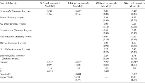
[image:10.612.59.554.412.698.2]Second, we drop the most likely candidate for a scale effect-driven response. Since 23% of the sample switches at the $10 row, we repeated the OLS and Tobit regressions of cost of delay on cross-modality and demographics but remove from the sample partici-pants that switch in this row. Table4reports the results of these regressions, showing that despite the smaller sample size, the cross-modal effect persists. The effect
Table 4. Influence of Cross-Modality on Cost of Delay, Excluding Those Who Switched for $10
Cost of delay ($) OLS excl. no-switch Tobit incl. no-switch OLS excl. no-switch Tobit incl. no-switch
Model (1) Model (2) Model (3) Model (4)
Cross-modal(dummy, 1yes) −3.90∗ −5.69∗∗∗ −3.89∗ −5.42∗∗
(1.86) (2.14) (2.03) (2.27)
Female(dummy, 1yes) 2.33 1.02
(1.91) (2.26)
Age at last birthday(years) −0.03 −0.15
(0.14) (0.16)
Low education(dummy, 1yes) −0.46 0.02
(3.33) (3.32)
High education(dummy, 1yes) −3.07 −0.09
(2.25) (2.62)
Married(dummy, 1yes) −0.28 −1.19
(2.94) (3.08)
Has children(dummy, 1yes) 0.27 3.43
(3.22) (3.50)
Employed full or part time −0.29 −1.78
(dummy, 1yes) (2.28) (2.74)
Constant 3.94∗∗∗ 6.24∗∗∗ 7.78∗∗ 10.74∗∗∗
(0.89) (1.50) (3.89) (4.10)
n 223 229 223 229
R2 0.019 0.037
Pseudo-R2 0.004 0.005
Sigma (Tobit) 16.18 — 16.08
(0.77) (1.17)
Notes. The terms “incl. no-switch” and “excl. no-switch” denote regressions including and excluding data from respondents who never switched, respectively. Where these data are included, Tobit regression allows for the truncation of the data. Robust standard errors are reported in parentheses.
∗p<0.10;∗∗p<0.05;∗∗∗p<0.01.
size is similar to that in Table 2, and the effect is sig-nificant at the 90% confidence level (at least) in all cases.
Discussion
So far we have made three contributions: we pre-sented a new preference measurement instrument, crystallised the implications of standard (value-based) theories for the relationship between unimodal and cross-modal intertemporal comparisons, and provided empirical findings at odds with the predictions of those theories. We now discuss how the DCM relates to stan-dard methods, explain how our baseline model is char-acteristic of value-based modelling approaches, and then take the first steps toward a view of preference that can explain our empirical finding.
Measurement Instrument. We have already stated the
main distinctive advantages of the DCM. But although the DCM departs from more traditional methods, such as eliciting an indifference point between smaller sooner and larger later sums of money, both the DCM and the traditional methods share the same core idea, which is that agents require compensation to accept the delay of an outcome, and this compensation provides a measure of time preference.
It is evident the DCM works on this principle, but it might be less clear how the more traditional methods do. Here, we demonstrate the commonality by show-ing how each task of the DCM can be reduced to the canonical task in two steps. In the first step, abolish the distinction betweent3 andt2, so that
compensa-tion is received at the same time as the later good. In the second step, make both the earlier and later good be the same fixed amount of money rather than dis-crete consumer goods. The good and the compensation are then in the same divisible units; the task elicits the adjustment to an initial sum of money that the partic-ipant requires to delay its receipt fromt1 to t2.
For example, a participant who is indifferent between $100 today and $120 in six months is revealing she will demand $20 compensation in six months to accept $100 in six months instead of $100 today.
The DCM is more general than the canonical task in that it achieves divisibility of compensation without requiring divisibility of goods. This permits the goods to be discrete and different from one another, so allow-ing for cross-modal comparisons and many other pos-sibilities, while leaving unaffected the core underlying idea about compensation as a measure of preference.
The Value-Based Modelling Approach. Earlier we used a baseline model to derive the hypothesis that the sum of cross-modal costs of delay equals the sum of unimodal costs of delay in the setup summarized by the Fisher diagram (see Figure1). A key assumption for this hypothesis was linearity of utility for the relevant money amounts. Linear utility is a standard assump-tion for small money amounts, but concavity is an obvi-ous alternative and has been proposed even for small amounts (e.g., Andersen et al. 2008, Andreoni and Sprenger2012, Galanter1962, Kahneman and Tversky
1979). In AppendixA, we show that assuming concav-ity does change the prediction of the baseline model. But this does not redeem the baseline model, because the change is in the opposite direction of what we observe.
As argued above, the baseline model is quite gen-eral when considered within the class of value-based accounts of intertemporal comparison. Nevertheless, it relies on the fundamental principle of the value-based approach, that the utility of a given dated good isindependent of its comparators. To see this, recall the argument that follows Equation (3) showing why, for an agent who prefers B1 to A2 and has v( · ) linear, [xAB −xAA] equals [xBB −xBA]. The argument is that each square-bracketed term is given by the difference in utility between the delayed goodsB2andA2. It rests on an implicit assumption that it does not matter to that difference whether these delayed goods are received instead ofA1(as they are for xAB and xAA)or instead ofB1(as they are forxBB andxBA). As this assumption is just an application of the fundamental principle, it
will typically carry over into other value-based mod-els. In view of this, we now explore explanations of our findings that depart from the value-based approach.
Explaining the Cross-Modal Effect. We provide two potential explanations for the discrepancy between cross-modal and unimodal choice that assume, respec-tively, that the weights put on option features and the interpretation of those options vary with what they are compared with. In the first explanation, which draws on insights from multiattribute choice (Houston and Sherman1995), the weight put on each attribute of an option is inversely related to how many attributes differ between those options. The second explanation draws on construal-level theory (Trope and Liberman 2003) and proposes that the mental representation of options depends on what they are compared to.
The first explanation treats the delay in intertempo-ral choices as only one attribute among many.14 All attributes, including delay, receive a decision weight that is directly related to their general importance and inversely related to the number of attributes that differ between options.15To illustrate the idea in an atempo-ral context, consider the value a consumer might place on the “color” attribute when valuing two used cars. Suppose this consumer will pay $100 more for a blue car than a red one when the cars differ only in color. Now suppose the cars differ in multiple attributes, such as model, engine size, mileage, age, and the upholstery on the seats. As these differences proliferate, the impact of color will likely decline until it plays little if any role in that consumer’s valuation of the cars. In general, as options become less similar in other respects, the weight on any differentiating attribute will decrease.16
We now briefly outline a model based on this intu-ition, which is elaborated and generalised in Ap-pendix B. Consider a stylised attribute specification of our four experimental options. Because the goods are either identical (in the unimodal comparisons) or very different (in the cross-modal), we capture the nature of the options as two elements in a vector, correspond-ing to the presence or absence of a particular good. The vector has an additional element for the timing of the good. If chocolates are the preferred good, a box of chocolates available now can be denoted as A1
(α,0, π), where the first element is nonzero because the
box of chocolates is present, and αdenotes the
atem-poral value of the chocolates. The second element is zero because the pen is absent (if present, we denote it as β), and the third isπ because the good is
avail-able now. Options are compared by first taking the difference between two option vectors and then the (possibly weighted) sum of the elements of the result-ing difference vector. This corresponds to the cogni-tive process of comparing options and computing their differences on each attribute. As an illustration, take two options—the chocolates now, A1(α,0, π), and
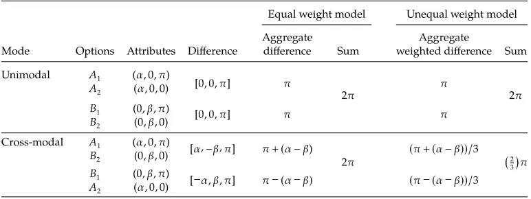
Table 5. Multiattribute Accounts of Cross-Modal and Unimodal Choices
Equal weight model Unequal weight model
Aggregate Aggregate
Mode Options Attributes Difference difference Sum weighted difference Sum Unimodal A1 (α,0, π) [0
,0, π] π π
A2 (α,0,0)
B1 (0, β, π) [0,0, π] π π
B2 (0, β,0)
2π 2π
Cross-modal A1 (α,0, π) [α,−β, π] π+(α−β) (π+(α−β))/3
B2 (0, β,0)
B1 (0, β, π) [−α, β, π] π− (α−β) (π− (α−β))/3
A2 (α,0,0)
2π 23π
the pen later,B2(0, β,0)—and compute the difference between them on each attribute,A1−B2[α,−β, π]. Provided each attribute is weighted equally, and using an additive specification, the strength of preference will follow the sum of these differences: the unweighted sum of the three elements is α−β+π. The relative
sizes ofα, β, andπare then enough to determine both
the choice betweenA1 and B2 and the compensation required to take the less preferred of the two. (AsA denotes the preferred good, α > β, and preference is
for A1, given any π >0. The compensation depends on all three terms.) This specification has an affinity with the baseline model in that combined strength of preference for both unimodal and cross-modal choices are the same as shown by the “Equal weight model” columns of Table5.
Suppose, however, our decision maker has limited attention and, as attribute differences proliferate, finds she has to spread that attention more thinly. The model detailed in Appendix B is based on the idea that a fixed quantity of attention is allocated over attributes that differ. Although the model is more general, a sim-ple instance is shown in the “Unequal weight model” column of Table5. In this instance, for the unimodal case, delay is the only attribute that differs, and so it receives a weight of one; in the cross-modal case, all three attributes vary, not only delay, and so each receives a weight of one-third. This leads the combined strength of preference (the final column of Table5) to be lower for cross-modal choices.
An additional and related explanation is that whether a choice is cross-modal or unimodal influ-ences the mental representation orconstrual of choice options. This extends the idea that the objects of choice are not defined by their physical properties but in their interpretation by the agent (e.g., Nisbett and Ross
1991), a notion that has received a substantial boost in the form of construal-level theory (Liberman and Trope
1998). To illustrate the idea, again imagine choosing between two cars, where car A is available now and car B later. When comparing the cars, we are likely to
define them in terms of features such as “color” and “leather seats.” Now imagine choosing between car A now and a vacation next year. We will certainly think of the two options differently—perhaps defining them in terms of their different purposes such as “transporta-tion” and “relaxation.” It would not be surprising if these different construals led to differences in the value placed on car A. Likewise, when choosing between chocolates now and later, our construal may be based on considerations such as the tastiness of the chocolates or how they melt in the mouth. This concrete represen-tation can promote a preference for earlier receipt of the good (Chen and He2011). By contrast, when making cross-modal choices we may care less about when the good is received, because we construe the options in terms of their more abstract and functional character-istics (perhaps improving a relationship, or writing a novel); see, e.g., Kim et al. (2013), Liberman and Trope (1998), and Liberman et al. (2002).
A study by Malkoc et al. (2010, Experiments 1A and 1B) also suggests that similarity between options, which is central to our distinction between cross-modal and unimodal choices, can influence patience, and does so by changing the way options are construed. Malkoc et al. did not elicit cross-modal and unimodal intertemporal choices, but rather elicited intertempo-ral choices after first having their participants make what we would call a “relatively unimodal” compari-son (a feature-by-feature comparicompari-son of two very sim-ilar digital cameras) and a “relatively cross-modal” comparison (between one of the digital cameras and a film camera with which it shared none of the specified features). After making the comparison, participants indicated how eager they were to receive a digital cam-era by indicating their WTA to agree to a 3- and 10-day delay in the delivery of that camera. Malkoc et al. found that participants were more sensitive to the delay when the initial comparison was (in our terminology) uni-modal rather than cross-uni-modal and also that that par-ticipants were generally more patient (although not significantly so) when a cross-modal evaluation had
preceded their choice. Malkoc et al. also observed that their participants construed the choice options more abstractly in their cross-modal-like comparison case, and that this difference in construal mediated the dif-ferences in patience in the two conditions.
The notion of “relative” cross-modality, hinted at in the above paragraph, brings in a broader issue. In our design the unimodal choices were between identi-cal objects and the cross-modal choices between radi-cally different objects. But there are many intermediate possibilities, such as choosing between a rescued cat from the animal shelter today or a pedigree cat from a litter yet to be born. Our experiment tested extreme cases, with delay the only attribute that varied between options in unimodal comparisons. As we have shown, such comparisons are likely to accentuate the impor-tance of time. A similar mechanism could be at work in canonical measures of time preference used in the previous literature. These measures vary two attributes (quantity and timing), which is fewer than the num-ber that would vary in many cross-modal decisions of everyday life. While there is much to learn about the role of time in complex decisions, our findings sug-gest that time does not have an absolute or predefined importance in decision making.
Acknowledgments
The authors thank the participants at the various conferences and workshops where this work was presented, and all the members of the Leverhulme Group at Warwick and the ESRC Network for Integrated Behavioural Science. Special thanks are due to Sudeep Bhatia, Andrea Isoni, George Loewenstein, and Robert Sugden, who all significantly influenced the authors’ thinking.
Appendix A. Further Analysis of the Baseline Model
In this appendix, we flesh out some details of the baseline model and extend it to cover the case where utility of money is nonlinear. We assume the agent’s decisions, taken at or before the start of t1, maximise the following objective
function, each component of which is a subutility function that is finitely valued and strictly increasing in all arguments:
Uu(A1,A2,B1,B2)+v( · ). (A.1)
This functional form imposes additive separability between dated goods and money, with utility from the former denoted by u( · ) and from the latter by v( · ). We impose that each dated good takes either the value 1 (indicating the agent receives it) or the value 0. Without further loss of generality, define the notation used in the main text as follows: u(1,0,0,0) ≡ a1; u(0,1,0,0) ≡a2; u(0,0,1,0) ≡b1; u(0,0,0,1) ≡b2. We normaliseu(0,0,0,0)to zero.
Following the default assumptions of the main text, we ignore indifference between dated goods and impose that
A1B1, A2B2, A1 A2, and B1 B2, with denoting
strict preference. This leaves open the preference overB1and
A2where considerations of preference over timing and
pref-erence over types of good can conflict. For brevity, in this appendix, we use the term “order TP” (for timing-based pref-erence) for the case whereB1A2and “order GP” (for
good-based preference) for the case whereA2B1.
The termsxAA,xBB, andxABare given by Equations (1.i)–
(1.iii) in the main text. For order TP,xBA is given by
Equa-tion (1.iv); for order GP,yBAis given by Equation (1.iv’). The
calculations in the main text demonstrate that, regardless of the functional form ofv( · ), Equation (2) holds under order TP and Equation (2’) under order GP. Whenv( · )is linear, Equations (2) and (2’) imply Equations (3) and (3’), respec-tively, which establish the null hypothesis of the baseline model. However, linearity ofv( · )is crucial for the transition from Equation (2) (respectively, (2’)) to Equation (3) (respec-tively, (3’)). The main task of this appendix is to show how the argument would be affected ifv( · )is strictly concave.
Take order TP first. It follows from its definition and the default assumptions that ∞>a1 >b1 >a2 >b2 >0. These
inequalities along with Equations (1.i)–(1.iv) imply that∞>
v(xAB)a1−b2>a1−a2v(xAA)>0 and∞>v(xBB)b1− b2>b1−a2v(xBA)>0, whereas Equation (2) yieldsv(xAB) − v(xAA)v(xBB)−v(xBA). Sincev( · )is strictly increasing, these
points imply that v(xAB) −v(xAA)and v(xBB) −v(xBA)are
equal increments to v( · ) induced by increases in its argu-ment, in one case from xAA to xAB and in the other case
from xBA toxBB. From Equations (1.iii) and (1.ii),v(xAB) a1−b2>b1−b2v(xBB). Consequently, withv( · )strictly
con-cave,xAB−xAA>xBB−xBA. Rearranging yieldsxAB+xBA> xAA+xBB. This inequality replaces Equation (3) whenv( · )is
concave and preference order TP applies.
Now consider order GP, with which (together with the default assumptions) implies∞>a1>a2>b1>b2>0 (NB: a2 andb1 are flipped relative to order TP). As a first step,
define the sum of moneyzsuch thatv(z)a1−b1and recall
thatv(0)0. From these points and Equations (1.ii)–(1.iii),
v(xAB) −v(z)b1−b2v(xBB) −v(0). Sincev( · )is increasing
andb1−b2>0, each of the termsv(xAB) −v(z)andv(xBB) − v(0) is an increment to v( · ) induced by an increase in its argument, in one case from ztoxAB and in the other case
from 0 to xBB; the two increments are equal since, as just
noted,v(xAB)−v(z)v(xBB)−v(0). Equations (1.ii)–(1.iii) also
imply v(xAB)a1−b2>b1−b2v(xBB). Combining these
conclusions, strict concavity ofv( · )implies
xAB−z>xBB−0. (A.2)
Now, using Equations (1.i) and (1.iv’),v(z) −v(xAA)a2− b1v(yBA)−v(0). Sincev( · )is increasing anda2−b1>0, each
of the termsv(z)−v(xAA)andv(yBA)−v(0)is an increment to v( · )induced by an increase in its argument, in one case from
xAA tozand in the other case from 0 to yBA. Moreover, as
just noted,v(z) −v(xAA)v(yBA) −v(0). Sincev(z)a1−b1> a2−b1v(yBA),v(z)>v(yBA). Combining these conclusions,
strict concavity ofv( · )implies
z−xAA>yBA−0. (A.3)
From (A.2) and (A.3),[xAB−z]+[z−xAA]>xBB+yBA.
Rear-ranging yieldsxAB−yBA>xAA+xBB. This inequality replaces
Equation (3’) whenv( · )is concave and preference order GP applies.
These arguments and those of the main text establish the following summarising result, which encapsulates all fea-tures of the baseline model needed for the paper.
Proposition 1. In the baseline model,
(i) xAB+xBA≥xAA+xBBfor preference order TP;
(ii) xAB−yBA≥xAA+xBBfor preference order GP; and
(iii) in both(i)and(ii), the weak inequality holds as an equality whenv( · )is linear and as a strict inequality whenv( · )is strictly concave.
This result shows that, provided each participant displays either preference order TP or preference order GP, concavity of v( · )cannot rationalise failure of the null hypothesis of the baseline model unless that failure takes the form that the combined cross-modal cost of delayexceedsthe combined
unimodal cost of delay. The opposite could, of course, be explained by convexity of v( · ), but that would be a very unusual assumption since we are only concerned withv( · )
in the domain of monetary gains.17
Appendix B. A Weighted Multiattribute Intertemporal Choice Model
Here, we provide a more general and formal account of the weighted multiattribute intertemporal choice model sketched in the main paper and illustrated in Table5, and we extend the argument to include explicit reference to mone-tary compensation. The model draws on ideas from a range of earlier researchers and has some formal properties in com-mon with the model of Kőszegi and Szeidl (2013). The model is specifically developed in the context of our experimental setup, and we do not claim greater generality for it.
The two goods and the two time periods are as in Figure1, yielding the same four dated goods. But now, as depicted in Table5, let there be three attributes on which a dated good can be evaluated: attribute 1 takes the valueαif the good to
be received is of typeAand 0 otherwise, attribute 2 takes the valueβif the good is of typeBand 0 otherwise, and attribute 3 takes the valueπif the good will be received int1 and 0 if it
will be received int2. We imposeα,β, andπ >0.18
For brevity, we address only the case where, in any com-parison between dated goods, the agent prefers the one with a sooner delivery date, denoted byS, over the one with the later delivery date, denoted byL. As in the main text, we use
xto denote WTA for taking the dispreferred option instead of the preferred one. The WTA is determined by the difference between the sums of weighted attributes for each option:
X r∈<
wr[Sr−Lr]v(x), (B.1)
wherev( · )is an increasing function defined on money;<is the set of attributes, with typical elementr. The termsSrand Lrare, respectively, the values ofSandLfor attributer; and wr is the weight put on attributerwhen comparingSandL.
Note that money is treated separately from other attributes to make its role as a measure of the “cost” of exchanges of dated goods clear. This makes the analysis simpler and comparable in this respect to the baseline model, without altering the key mechanism that we model. It does differ formally, however, from previous attribute-based choice models of time prefer-ence where money is treated similar to other attributes (e.g., Scholten and Read2010).
The weight put on each attribute is a function of the abso-lute difference between the two options on that attribute and the sum of those absolute differences for all attributes where the two options differ. That is, for any attributer∈ <,
wrg(|Sr−Lr|) . X
r0∈<0
g(Dr0), (B.2)
where<0is the subset of<containing those attributes where
SandLtake different values,Dr0is the maximum (in abso-lute value) difference in values possible on attributer0∈ <0, and g( · ) is an increasing function with g(0)0. The
for-mulation (B.2) imposes no restrictions on the relative sizes of g(α), g(β), and g(π), leaving the decision maker free to regard any attribute as “intrinsically” more important than any other. However, an attribute for which S and L take the same value has no bearing on the choice between them. Instead, a total decision weight of unity is spread across those attributes whereSandLdiffer in proportions determined by their intrinsic importance. (This generalises the case consid-ered in Table5.)
In the value-vector form,A1(α,0, π),A2(α,0,0),B1 (0, β, π), andB2(0, β,0). As in the main text, we let good Abe the preferred good. To ensure this and that, in every intertemporal comparison, the earlier option is preferred to the later one, it suffices to imposeπg(π)> αg(α) −βg(β)>0.
Then,xAAandxBBare defined implicitly by
[πg(π)/g(π)]v(xAA), (B.3)
[πg(π)/g(π)]v(xBB), (B.4)
i.e., by πv(xAA)v(xBB). It is an immediate implication
thatxAAxBB. Note, however, that this implication would be
relaxed had we allowed different delay attributes for different goods.
For brevity, we denote the sum g(α)+g(β)+g(π)asΩ.
ThenxABsatisfies
[πg(π)+(αg(α) −βg(β))]/Ωv(xAB). (B.5)
Similarly,xBAsatisfies
[πg(π) − (αg(α) −βg(β))]/Ωv(xBA). (B.6)
We now work out the implications of these implicit defini-tions for the reladefini-tionship between cross-modal and unimodal WTAs. First, supposev(x)x. Then,
xAA+xBB2π (B.7)
and
xAB+xBA[2πg(π)/Ω]. (B.8)
Thus,xAA+xBB>xAB+xBA, because the ratiog(π)/Ω, which
we will call thecross-modal deflator, is less than unity. By a
trivial extension of the argument, xAA+xBB>xAB+xBA is
guaranteed for any linearv( · ).
Now, supposev( · )is concave. From Equations (B.3) and (B.4),v(xAA)andv(xBB)each takes the valueπ. Relative to this,
the value ofv(xBA)in (B.6) is deflated in two ways. First,πis
deflated by the cross-modal deflatorg(π)/Ω; then the result is
further reduced by subtracting(αg(α) −βg(β))/Ω(>0)from it. Sincev( · )is increasing, it follows that each ofxAAandxBB
exceedsxBA. By contrast, relative to v(xAA)and v(xBB), the