Sparse Modeling Using Orthogonal Forward
Regression With PRESS Statistic and Regularization
Sheng Chen
, Senior Member, IEEE
, Xia Hong
, Senior Member, IEEE
, Chris J. Harris, and Paul M. Sharkey
Abstract—The paper introduces an efficient construction algo-rithm for obtaining sparse linear-in-the-weights regression models based on an approach of directly optimizing model generalization capability. This is achieved by utilizing the delete-1 cross validation concept and the associated leave-one-out test error also known as the predicted residual sums of squares (PRESS) statistic, without resorting to any other validation data set for model evaluation in the model construction process. Computational efficiency is en-sured using an orthogonal forward regression, but the algorithm incrementally minimizes the PRESS statistic instead of the usual sum of the squared training errors. A local regularization method can naturally be incorporated into the model selection procedure to further enforce model sparsity. The proposed algorithm is fully automatic, and the user is not required to specify any criterion to terminate the model construction procedure. Comparisons with some of the existing state-of-art modeling methods are given, and several examples are included to demonstrate the ability of the pro-posed algorithm to effectively construct sparse models that gener-alize well.
Index Terms—Bayesian learning, cross validation, orthogonal forward regression, predicted residual sums of squares (PRESS) statistic, regularization, sparse data modeling.
I. INTRODUCTION
T
HE objective of modeling from data is not that the model simply fits the training data well. Rather, the goodness of a model is characterized by its generalization capability, inter-pretability and ease for knowledge extraction. Note that all these properties depend crucially on the ability to construct appro-priate sparse models by the modeling process, and a basic prin-ciple in practical nonlinear data modeling is the parsimonious principle that ensures the smallest possible model that explains the training data. There exists a vast amount of works in the area of sparse modeling (e.g., [1]–[9]). Recently, a well-known sparse kernel modeling algorithm has perhaps been the support vector machine (SVM) method [8], which is widely regarded as the state-of-art technique for regression and classification ap-plications. The formulation of SVM embodies the structural risk minimization principle, thus combining excellent generalization properties with a sparse model representation. Despite these at-tractive features and many good empirical results obtained using the SVM method, data modeling practicians have realized that the ability for the SVM method to produce sparse models hasManuscript received December 5, 2002; revised March 20, 2003. This paper was recommended by Associate Editor M. Berthold
S. Chen and C. J. Harris are with Department of Electronics and Computer Science, University of Southampton, Southampton SO17 1BJ, U.K.
X. Hong and P. M. Sharkey are with Department of Cybernetics, University of Reading, Reading RG6 6AY, U.K.
Digital Object Identifier 10.1109/TSMCB.2003.817107
perhaps been overstated. This has motivated Tipping [9] to in-troduce the relevance vector machine (RVM) method.
The RVM method adopts a Bayesian learning framework [4]. The introduction of individual hyperparameters for every weights of the regression model is the key feature of the RVM method and is ultimately responsible for the sparsity properties of the RVM method [9]. An evidence procedure [4] is used to iteratively optimize kernel weights and the associated hyperparameters. During the optimization process, many of these hyperparameters are driven to large values so that the corresponding model weights are effectively forced to be zero and their associated model terms can then be removed from the trained model. The results given in [9] have demonstrated that the RVM has a comparable generalization performance to the SVM but requires dramatically fewer kernel functions or model terms than the SVM. A drawback of the RVM method is a significant increase in computational complexity, compared with the SVM method. A more serious limitation is however inherent in the evidence framework. The compu-tation of the associated Hessian matrix required for updating hyperparameters is expensive, and this Hessian matrix may be near singular or singular and thus noninvertible. At a local minimum, some eigenvalues of this Hessian matrix may even be negative [10] and thus cause numerical instability for the iterative optimization procedure.
The orthogonal least squares (OLS) algorithm [1], which was developed in the late 1980s for nonlinear system modeling, remains popular for nonlinear data modeling practicians because the algorithm is simple and efficient and is capable of producing parsimonious linear-in-the-weights nonlinear models with good generalization performance. Over time, many “improved” variants of the OLS algorithm have been proposed [11]–[16]. In particular, the locally regularized OLS (LROLS) algorithm [13], [15] has been shown to be capable of producing very sparse regression models that generalize well. The key idea of the LROLS algorithm is in fact adopted from the RVM method, namely using the multiple regularizers to enforce sparsity. The LROLS algorithm is, however, based on the forward selection principle, has the ability to reveal the significance of individual model regressor, and only selects those significant terms, whereas the RVM method starts with the full model set and is effectively based on the backward elimination principle. It is well known that forward selection is computationally more attractive compared with backward elimination. More importantly, in the LROLS algorithm, only a subset matrix of the full Hessian matrix is used. This subset matrix is diagonal and well-conditioned with small eigenvalue spread. Therefore, the inverse of the Hessian is trivial, the
regularization parameter updating is exact and simple, and the iterative procedure converges fast.
As in most model construction algorithms, the criterion used by the OLS algorithm in the model construction process is the training mean square error (MSE). Since the training MSE typically decreases as the model size increases, a separate stopping criterion is needed to stop the selection procedure in order to avoid an over-fitted model. For example, infor-mation-based criteria, such as the AIC and the minimum description length [17]–[19], can be adopted to terminate the model selection process. An information based criterion can be viewed as a model structure regularization by using a penalty term to penalize large-sized models. However, the penalty term in an information based criterion does not determine which model term should be selected. Multiple regularizers, i.e., local regularization [9], [13], [15], and optimal experimental design criteria [14] offer better solutions as model structure regularization as they are directly linked to model efficiency and parameter robustness. The underlying “problem,” however, remains that the basic criterion for most model construction procedures is the training MSE. Arguably, a better and more natural approach is using a criterion of model generalization capability directly in the model selection procedure rather than only using it as a measure of model complexity.
The evaluation of model generalization capability is directly based on the concept of cross validation [20]. This paper inves-tigates a model construction algorithm using a model selection criterion that is based explicitly on cross validation. This is achieved with a training data set only by utilizing the concept of delete-1 cross validation and the associated leave-one-out test error also known as the predicted residual sums of squares (PRESS) statistic [21]–[23]. The use of the leave-one-out estimate for general nonlinear-in-the-weights models has been studied in [24]–[26]. Even for the class of linear-in-the-weights models, computation of the mean square PRESS error is normally expensive and the use of the PRESS statistic in model selection is generally prohibitive. However, a recent study [27] has shown that, using the OLS algorithm, the calculation of the PRESS statistic becomes efficient and model selection based on the PRESS statistic is computationally affordable. It is well known that local regularization is effective in enforcing model sparsity as well as ensuring excellent generalization performance [9], [13], [15]. We combine the PRESS statistic with local regularization in the orthogonal forward regression procedure. The resulting algorithm selects a sparse model by incrementally minimizing a regularized mean square PRESS error.
Our motivation is twofold. First, we aim to derive a construc-tion algorithm based directly on optimizing model generaliza-tion capability, without resorting to use a separate validageneraliza-tion data set. We also want the model construction process to be au-tomatic without the need for the user to specify some additional terminating criterion. The usual training MSE cannot achieve these objectives, but the PRESS statistic provides the capability to do so. Second, the level of sparsity and computational effi-ciency are also critical to the model construction process, and the LROLS algorithm (based on the training MSE) is known
to offer considerable advantages in these two aspects. By com-bining the PRESS statistic with the LROLS algorithm, we ob-tain a truly automatic and computationally efficient construc-tion algorithm capable of producing very sparse models with excellent generalization performance, using a training data set only. Several illustrative examples are included to illustrate the effectiveness of this approach. Comparisons with some of the existing state-of-art modeling methods are given, and the re-sults demonstrate that our LROLS algorithm based on PRESS statistic compares favorably in terms of achieving the above-stated objectives.
II. LINEAR-IN-THE-WEIGHTSREGRESSIONMODEL
Consider the general discrete-time nonlinear system repre-sented by the nonlinear model [28]
(1)
where and are the system input and output variables with integers and representing the lags in and , respectively, is a white noise,
denotes the system “input” vector, and is the unknown system mapping. The system (1) is to be identified from an -sample observation data set
using some suitable functional that can ap-proximate with arbitrary accuracy. One class of such func-tionals is the regression model of the form
(2)
where denotes the model output, are the model weights, are the regressors and
with , and is the
total number of candidate regressors. The model (2) is very general and includes all the kernel-based models, the polyno-mial-expansion model [1], and the general linear-in-the-weights nonlinear model [29]. In particular, for kernel-based models, the regressor takes the form
(3)
where is the kernel center, and is a given kernel function.
By letting , for ,
and defining and
, the regression model (2) can be written as
(4)
Let an orthogonal decomposition of the matrix be
where
. .. ... ..
. . .. ...
(6)
and
(7)
with columns satisfying , if . The regression model (4) can alternatively be expressed as
(8)
where the orthogonal weight vector sat-isfies the triangular system . The space spanned by the original model bases ,] is identical to the space spanned by the orthogonal model bases
, and the model is equivalently expressed by
(9)
where .
III. OLS ALGORITHMBASED ONPRESS STATISTIC AND
LOCALREGULARIZATION
A. Model Selection Using Cross Validation With PRESS Statistic
Consider the model selection problem where a set of models or predictors have been identified using the training data set . Denote these predictors, identified using all the
data points of , as with index .
Cross validation using the stacked regression combines these models to achieve better generalization performance [22], [23]. Our aim here is to select a single parsimonious model with good generalization capability. To optimize generalization capability, cross validation is often used for model selection [20]. A commonly used cross validation is the delete-1 cross validation. The idea is as follows. For every predictor, each data point in the training set is sequentially set aside in turn, a model is estimated using the remaining data points, and the prediction error is derived using only the data point that was removed from training. Specifically, let be the resulting data set by removing the th data point from , and denote the th model estimated using as and the related predicted model residual at as
(10)
The leave-one-out test error or the mean square PRESS error [21], [24] for the th model is obtained by averaging all these prediction errors:
(11)
To select the best predictor from the candidate predictors , the same modeling procedure is applied to each of the predictors, and the predictor with the minimum PRESS statistic is selected.
For linear-in-the-weights models, the PRESS statistic can be generated, without actually sequentially splitting the training data set and repeatedly estimating the associated models, by using the Sherman–Morrison–Woodbury theorem [21]. Consider that an -term model is identified using based on the model form of (2). The PRESS errors are calculated using [21], [24]
(12)
where . The computation of the
PRESS error in (12) relies on the assumption that the regression matrix has full rank. Obviously, choosing the best subset model that minimizes the PRESS statistic quickly becomes computationally prohibitive even for a modest -term model set. Moreover, the PRESS error (12) itself is computational expensive because the matrix inversion involved. However, if we choose only to incrementally minimize the PRESS statistic in an orthogonal forward regression manner, as presented in [27], the model selection procedure based on the PRESS statistic becomes computationally affordable. Furthermore, due to orthogonalization, the calculation of the PRESS errors becomes very efficient [27]. Note that the orthogonal forward selection procedure will always select a subset model such that the associated Hessian matrix is not only diagonal but well conditioned as well.
B. LROLS Algorithm Based on PRESS Statistic
The LROLS algorithm [13], [15] is based on the following regularized training error criterion
(13)
where is the regularization parameter
vector, and diag . The algorithm selects a subset model by incrementally minimizing the regularized training MSE. As is defined in [13] and [15], the regularized error reduction ratio due to the regressor is given by
rerr (14)
At the th stage of selection procedure, a model term is selected if it produces the largest regularized error reduction ratio among the remaining to candidates. The selection process is ter-minated at the th stage if
rerr (15)
The regularization parameters can be optimized iteratively using an evidence procedure [4], [9]. The following error cri-terion is obviously equivalent to the cricri-terion (13):
(16)
where is the noise parameter (inverse of noise variance), is the hyperparameter vector, and diag . The relationship between a regu-larization parameter and its corresponding hyperparameter is given by
(17)
It can be shown that the log evidence for and is [4]
evidence
constant (18)
Because of the orthogonalization, the Hessian matrix is diag-onal and is given by
diag
(19)
Setting the derivatives of evidence with respect to and to zeros yields the updating formulas for and , respectively. Substituting these updating formulas into (17) results in the up-dating formulas for the regularization parameters:
(20)
where
and (21)
Usually a few iterations (typically less than 10) are sufficient to find a (near) optimal .
In the orthogonal forward selection procedure, if is too small (near zero), this term will not be selected. This build-in mechanism automatically avoids any ill-conditioning situations. For the original OLS algorithm [1], the value of the user spec-ified terminating scalar is critical for avoiding an overfitted model. For the above LROLS algorithm based on training MSE, the choice of is less critical, as is shown in [13] and [15]. Nev-ertheless, the user is still required to specify an appropriate value for . The main component in the model selection criterion for the above algorithm is the training MSE. We can modify the model selection procedure so that the subset model selection is based entirely on the model generalization capability. Specif-ically, we use the PRESS statistic as the subset model selec-tion criterion, whereas the model parameter estimate and the
up-date of regularization parameters remain the same as the above LROLS algorithm.
Using the equivalent orthogonal model (9) and incorporating parameter regularization, the PRESS error is given by
(22)
where the PRESS error weighting is given by
(23)
The derivation of (22) is similar to the case without regulariza-tion given in [27]. The mean square PRESS error for the model with a size is then given by
(24)
Note that the model residual for the -term model can be computed recursively as
(25)
and similarly, the PRESS error weighting can be written in a recursive formula by
(26)
The recursive formulas (25) and (26) enable an efficient com-putation of the PRESS statistic (24).
The subset model selection procedure can be modified as fol-lows. At the th stage of the selection procedure, a model term is selected among the remaining to candidates if the re-sulting -term model produces the smallest mean square PRESS error. It has been shown in [27] that the PRESS statistic is concave with respect to the model size . That is, there exists an “optimal” model size such that for , decreases as increases, whereas for , increases as increases. Thus, the selection procedure is automatically terminated with an -term model when , without the need for the user to specify a separate termination criterion. The iterative model selection procedure based on the LROLS algorithm with PRESS statistic can now be summarized.
1) Initialization: Set , to the same small positive value (e.g., 0.000 01). Set iteration .
Step 1) Given the current and with the following initial conditions:
and
use the procedure described in the Appendix to se-lect a subset model with terms.
Step 2) Update using (20) and (21) with . If remains sufficiently unchanged in two successive iterations or a preset maximum iteration number is reached, stop; otherwise, set , and go to Step 1.
The requirements of computing the PRESS statistic in the selection process represent a considerable complexity increase, compared with the LROLS algorithm using the regularized training MSE. However, the computational complexity of the proposed algorithm is clearly affordable, due to the orthogonal forward regression and, in particular, the efficient recursive calculation of the PRESS errors. The main advantage of the proposed algorithm is that the model selection is directly based on the model generalization capability. Therefore, even without regularization, the algorithm, which is first derived in [27], is capable of producing sparse models with excellent generalization performance. The local regularization can often further enforce sparsity to derive much sparser models in many practical modeling situations. These observations will be illustrated later on by some modeling examples.
IV. COMPARISON WITHSOMEEXISTINGMODEL
CONSTRUCTIONALGORITHMS
Several model construction algorithms are used for a compar-ison with the proposed LROLS algorithm with PRESS statistic, and they are the OLS algorithm with PRESS statistic [27], the LROLS algorithm with regularized training MSE [13], [15], the RVM algorithm [9], and the enhanced -means clustering and least squares (CLS) algorithm [30], [31]. The OLS with PRESS statistic and the LROLS with PRESS statistic are both automatic construction algorithms using only a training data set. It should be pointed out that the computational complexity of the LROLS algorithm is not necessarily significantly more than that of the OLS algorithm, even though the former involves an iterative loop. This is because typically after the first iteration, which has a complexity of the OLS algorithm, the model set contains only terms, and the complexity of the subsequent itera-tion decreases dramatically. The LROLS algorithm with training MSE has a complexity less than that of the LROLS algorithm with PRESS statistic, and it is also an automatic construction algorithm using only a training data set, provided that an ap-propriate value for can be specified. When an appropriate cannot be found, it may then be necessary to use other termi-nating criteria, such as employing an additional validation data set.
The RVM algorithm [9] shares certain common features with the LROLS algorithm, as they both use an approach of mul-tiple regularizers to enforce sparsity and adopt a similar evi-dence procedure for updating hyperparameters or regularization parameters. It is therefore not surprising that the generalization capabilities and the levels of sparsity provided by the two algo-rithms are similar. The LROLS algorithm, however, has consid-erable computational advantages in that it can operate robustly in difficult modeling conditions, and its iterative loop generally converges faster compared with the RVM (see the discussion in
[15]). Using the equivalent regularization formula, the RVM for regression [9] can be reformulated to involve an iterative loop of the model weight estimation and regularization parameter up-dating. With given , the model weight estimate is the regular-ized least squares (LS) solution:
(28)
where the Hessian matrix is given by
(29)
The regularization parameters are updated using
(30)
where
with (31)
and denotes the th diagonal element of . The RVM starts with the full model set and removes those regressors that have large values in their associated regularization param-eters. Clearly, the inverse of is expensive and this matrix may be ill-conditioned or even singular. Compared with the LROLS algorithm, the regularization parameter updating is much more expensive, and the iterative procedure generally converges with slower rate and may suffer from numerical instability. Model pruning in the RVM method is done by specifying a large threshold . If a model term with its associated regularization parameter satisfying , it is removed. During the iterative procedure, may need to be reduced gradually in order to derive an appropriate final sparse model. Provided that can be set appropriately and numerical instability does not occur, the RVM algorithm can provide a very sparse model with excellent generalization performance using only a training data set.
process to seek the kernel centers . The enhanced -means clustering algorithm [35] is summarized as follows:
(32)
where is a learning rate, the membership function is defined as
if for all
otherwise
(33)
and is the variation or “variance” of the th cluster. To estimate variation , the following updating rule is used:
(34)
where is a constant slightly less than 1.0. The initial varia-tions are set to the same small number. Note that the learning rate can be self-adjusting based on an “entropy” formula [35]
(35)
where
with
(36)
Given the set of kernel centers , the kernel model in the form (2) can be formed, and the model weight vector is readily given by the LS solution . The enhanced CLS algorithm has a very low complexity. However, the algorithm itself does not provide the required number of cluster prototypes or model terms for adequately modeling the data, i.e., it cannot determine the model structure. We will adopt a practical strategy of having a separate validation data set at a cost of increasing complexity. A range of models with different model sizes are fitted to the training data set, and the MSE values of the fitted models are computed over the validation set. The model with a size , which has the smallest test MSE, is selected.
V. MODELLINGEXAMPLES
Example 1: This example used a radial basis function (RBF) network to model the scalar function
(37)
Four hundred training data were generated from , where the input was uniformly distributed in , and the noise was Gaussian with zero mean and standard deviation 0.2. The first 200 data points were used for training and the other 200 samples for model validation. The RBF model employed the Gaussian kernel function of the form
[image:6.612.321.532.63.207.2](38)
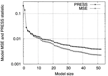
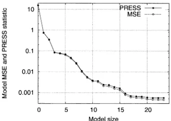
[image:6.612.335.519.255.363.2]Fig. 1. Evolution of training MSE and PRESS statistic versus model size for simple scalar function modeling problem using the OLS algorithm based on PRESS statistic without the help of a validation set.
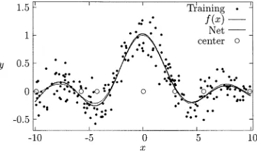
Fig. 2. Simple scalar function modeling problem. (Dots) Noisy training data
y. (Thin curve) Underlying functionf(x). (Thick curve) Model mapping. (Circles) Selected RBF centers. The seven-term model was identified by the OLS algorithm based on PRESS statistic without the help of a validation set.
where was the th RBF center vector and the kernel vari-ance. For this example, was found to be optimal empirically and was used for all the models. As each training data was considered as a candidate RBF center, there were regressors in the regression model (2). The training data were very noisy. Two hundred noise-free data with equally spaced in were also generated as an addi-tional testing data set for evaluating model performance.
We first applied the OLS algorithm based on PRESS statistic. Fig. 1 depicts the evolution of the training MSE and PRESS statistic in scale during the forward regression procedure with a typical set of noisy training data set. It can be seen that the PRESS statistic continuously decreased until
, and the algorithm terminated with a seven-term model. The training MSE, the mean square PRESS error, and the MSEs over the noisy and noise-free testing sets, respectively, for the constructed seven-term model are summarized in Table I. Fig. 2 shows the noisy training points and the underlying func-tion together with the mapping generated using the model identified by the OLS algorithm based on PRESS statistic. It can be seen from the results shown in Table I and Fig. 2 that the OLS algorithm based on PRESS statistic automatically identi-fied a very sparse model from the noisy training data set with excellent generalization capability.
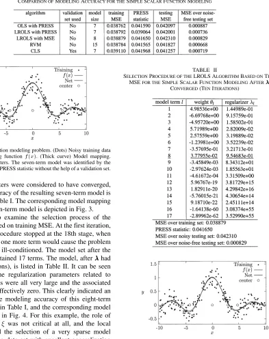
TABLE I
[image:7.612.129.522.76.572.2]COMPARISON OFMODELINGACCURACY FOR THESIMPLESCALARFUNCTIONMODELING
Fig. 3. Simple scalar function modeling problem. (Dots) Noisy training data
y. (Thin curve) Underlying function f(x). (Thick curve) Model mapping. (Circles) Selected RBF centers. The seven-term model was identified by the LROLS algorithm based on PRESS statistic without the help of a validation set.
regularization parameters were considered to have converged, and the modeling accuracy of the resulting seven-term model is also summarized in Table I. The corresponding model mapping generated by this seven-term model is depicted in Fig. 3.
It is informative to examine the selection process of the LROLS algorithm based on training MSE. At the first iteration, the model selection procedure stopped at the 18th stage, when it detected that adding one more term would cause the problem to be singular or very ill-conditioned. The model set after the first iteration thus contained 17 terms. The model, after had converged (ten iterations), is listed in Table II. It can be seen from Table II that the regularization parameters related to the ninth to 17th terms were all very large and the associated model weights were effectively zero. This clearly indicated an eight-term model. The modeling accuracy of this eight-term model is summarized in Table I, and the corresponding model mapping is illustrated in Fig. 4. For this example, the role of terminating threshold was not critical at all, and the local regularization enabled the selection of a very sparse model from the noisy training data set with excellent generalization capability.
For the RVM algorithm, the iterative process was observed to converge slower, and 50 iterations were required. The pruning threshold was initially set to , which was sub-sequently reduced to 500.0 at the tenth iteration, to 4.5 at the 30th iteration, and to 0.05 at the 40th iteration. The construction process produced a 15-term model as listed in Table III, and the modeling accuracy of this model can be seen in Table I. Fig. 5 depicts the model mapping generated by this 15-term model, where it can be observed that some of the selected centers were very close to each other and a seven-term model was in fact possible, but there existed no mechanism within the RVM algo-rithm to find this very sparse seven-term model that would have the same excellent generalization performance as the 15-term model shown in Table III.
TABLE II
SELECTIONPROCEDURE OF THELROLS ALGORITHMBASED ONTRAINING
MSEFOR THESIMPLESCALARFUNCTIONMODELINGAFTERHAS
CONVERGED(TENITERATIONS)
Fig. 4. Simple scalar function modeling problem. (Dots) Noisy training data
y. (Thin curve) Underlying function f(x). (Thick curve) Model mapping. (Circles) Selected RBF centers. The eight-term model was identified by the LROLS algorithm based on the training MSE without the help of a validation set.
TABLE III
MODELCONSTRUCTED BY THERVM ALGORITHM FOR THESIMPLESCALAR
FUNCTIONMODELINGAFTERHASCONVERGED(50 ITERATIONS)
Fig. 5. Simple scalar function modeling problem. (Dots) Noisy training data
y. (Thin curve) Underlying function f(x). (Thick curve) Model mapping. (Circles) Selected RBF centers. The 15-term model was identified by the RVM algorithm without the help of a validation set.
Fig. 6. Training and testing MSE values over the training and validation sets, respectively, versus model size for simple scalar function modeling problem using the enhanced CLS algorithm with the help of a validation set.
[image:8.612.72.256.97.384.2]Example 2: This was a simulated nonlinear dynamic con-trol system considered in [36]. The underlying dynamic system was governed by (39), shown at the bottom of the next page, where the system input was a random signal uniformly distributed in the interval . The noisy system output was
Fig. 7. Simple scalar function modeling problem. (Dots) Noisy training data
[image:8.612.340.516.227.351.2]y. (Thin curve) Underlying functionf(x). (Thick curve) Model mapping. (Circles) Selected RBF centers. The seven-term model was identified by the enhanced CLS algorithm with the help of a validation set.
Fig. 8. Evolution of training MSE and PRESS statistic versus model size for simulated control system modeling problem using the OLS algorithm based on PRESS statistic without the help of a validation set.
given by , where the noise was Gaussian with zero mean and standard deviation 0.05. Four hundred noisy samples were generated. The first 200 data points were used for training, and the other 200 samples were used for model valida-tion. A RBF network with the thin-plate-spline basis function
(40)
and the input vector
(41)
[image:8.612.74.257.441.568.2]was used to construct a model from the noisy training data set. As each training data point was considered as a candidate RBF center, there were candidate regressors.
Fig. 8 illustrates the evolution of the training MSE and PRESS statistic for the OLS algorithm based on PRESS statistic, where it can be seen that the PRESS statistic
contin-uously decreased until ,
and the algorithm terminated with a 51-term model. For the LROLS algorithm based on PRESS statistic, the model set was reduced to a size of 51 after the first iteration, and a constant size of 31 terms was reached after a few iterations. The final 31-term model was produced after 20 iterations. For the LROLS algorithm based on training MSE, it was found that as
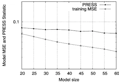
Fig. 9. Training and testing MSE values over the training and validation sets, respectively, versus subset model size for simulated control system modeling problem using the LROLS algorithm based on training MSE with the help of a validation set.
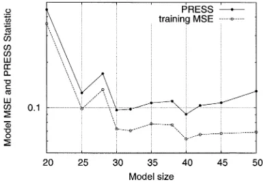
Fig. 10. Training and testing MSE values over the training and validation sets, respectively, versus model size for simulated control system modeling problem using the enhanced CLS algorithm with the help of a validation set.
more terms were added the training MSE kept decreasing and the corresponding regularization parameters all had reasonable small values. Thus, it was difficult to determine an adequate sparse model by specifying an appropriate value for , and it was decided to use the validation data set to help the model construction. Fig. 9 depicts the training and testing MSE values versus the subset model size, and the result appeared to suggest a 42-term subset model. For the RVM algorithm, 60 iterations were used, and the pruning threshold was initially set to which was subsequently reduced to 0.25 at the 50th iteration. With this choice of , the RVM method was able to construct a 42-term model without the need of employing the validation set. For the enhanced CLS algorithm, was used with 60 passes of the training data set for clustering. The model structure determination with the help of the validation set is depicted in Fig. 10, where a decision was made to choose the 49-term model.
The five models produced by the five algorithms are com-pared in Table IV. The constructed RBF model was used to iteratively generate the model output according to
(42)
with the input vector given by
(43)
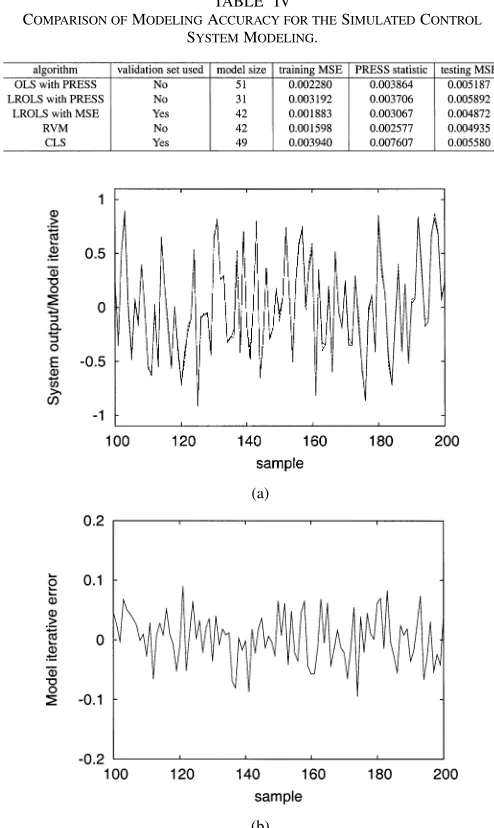
TABLE IV
COMPARISON OFMODELINGACCURACY FOR THESIMULATEDCONTROL
SYSTEMMODELING.
(a)
(b)
Fig. 11. Modeling performance for simulated control system modeling problem. (a) Iterative model output^y (k)(dashed) superimposed on system outputy(k)(solid). (b) Iterative model error (k). The 42-term model was constructed by the RVM algorithm without the help of a validation set.
Fig. 11 plots the iterative model output and error
for the 42-term model constructed by the RVM algorithm. The other four model responses, which are not shown here, were all similar to the results shown in Fig. 11. The results demonstrate that the five constructed models were adequate and had similar generalization capability. For this example, the OLS with PRESS, the LROLS with PRESS, and the RVM were able to automatically construct sparse models without the help of a validation set, and in particular, the LROLS algorithm based on PRESS statistic resulted in a much sparser model, compared with the other four algorithms.
[image:9.612.63.270.259.401.2](a)
[image:10.612.340.514.61.184.2](b)
Fig. 12. Engine data set (a) inputu(k)and (b) outputy(k).
data set, which is depicted in Fig. 12, contained 410 samples. The first 210 data points were used in modeling and the last 200 points in model validation. A RBF model with the input vector
(44)
and the Gaussian basis function of variance 1.69 was used to model the data. As each in the training data set was con-sidered as a candidate RBF center, there were can-didate regressors. From Fig. 12, it is seen that a strong periodic component was presented in the data, and this was believed to have caused numerical problem for the RVM method during the modeling construction.
[image:10.612.79.248.62.317.2]Fig. 13 shows the evolution of the training MSE and PRESS statistic for the OLS algorithm based on PRESS statistic. For this example, the algorithm resulted in a sparse 22-term model. For the LROLS algorithm based on PRESS statistic, the model set contained 22 terms after the first iteration, and the subse-quent iterations did not reduce the model set any further. The final 22-term model was obtained after ten iterations. For the LROLS algorithm based on training MSE, during the first iter-ation, the model selection procedure stopped at the 55th stage to avoid the singular or very ill-conditioning problem. By exam-ining the 54-term model obtained after ten iterations, it was seen that the 35th to 54th terms had large values of associated with them. Thus, the algorithm was able to produce a sparse 34-term model using only the training data set and without the need to specify an appropriate value for . Note that if the validation set was used to help determining the model structure, a sparser model with 23 terms was obtained with the same generalization performance as the 34-term model. For the enhanced CLS algo-rithm, the clustering algorithm passed through the training data set 50 times with . The model structure determination with the aid of the validation set is illustrated in Fig. 14, and the result suggested a 23-term model.
Fig. 13. Evolution of training MSE and PRESS statistic versus model size for engine data set modeling problem using the OLS algorithm based on PRESS statistic without the help of a validation set.
Fig. 14. Training and testing MSE values over the training and validation sets, respectively, versus model size for engine data set modeling problem using the enhanced CLS algorithm with the help of a validation set.
The modeling accuracies of the four resulting models are compared in Table V, where it can be seen that the four models have similarly good generalization performance. The constructed RBF model was used to generate the model prediction according to
(45)
with the input vector given by (44). Fig. 15 depicts the model prediction and the prediction error
for the 22-term model constructed by the LROLS algo-rithm based on PRESS statistic. The other three models have similar prediction performance to the results shown in Fig. 15.
For this example, the RVM algorithm as implemented in the form given in Section IV failed to work due to numerical insta-bility of the iterative loop for updating regularization parame-ters. Various initial values for were tried and a more stable updating formula for
(46)
[image:10.612.324.529.234.379.2]TABLE V
COMPARISON OFMODELINGACCURACY FOR THEENGINEDATASET
(a)
(b)
Fig. 15. Modeling performance for engine data set modeling problem. (a) Model prediction^y(k)(dashed) superimposed on system outputy(k)(solid). (b) Model prediction error(k). The 22-term model was constructed by the LROLS algorithm based on PRESS statistic without the help of a validation set.
which can affect the algorithm’s performance in adverse mod-eling environments.
Example 4: This example constructed a model for the gas furnace data set [38, ser. J]. The data set contained 296 pairs of input–output points, where the input was the coded input gas feed rate and the output represented CO concentra-tion from the gas furnace. All the 296 data points were used in training. A RBF network with the input vector
(47)
and the thin-plate-spline basis function was used to fit the data set. The number of candidate regressors in the regression model
(2) was .
The OLS algorithm based on PRESS statistic terminated the model construction with a sparse 32-term model when the
[image:11.612.330.523.344.478.2]con-dition was reached, and
Fig. 16. Evolution of training MSE and PRESS statistic versus model size for gas furnace data set modeling problem by the OLS algorithm based on PRESS statistic using the training data set.
Fig. 17. Evolution of training MSE and PRESS statistic versus model size for gas furnace data set modeling problem by the LROLS algorithm based on training MSE using the training data set.
Fig. 18. Evolution of training MSE and PRESS statistic versus model size for gas furnace data set modeling problem by the enhanced CLS algorithm using the training data set.
TABLE VI
COMPARISON OFMODELINGACCURACY FOR THEGASFURNACEDATASET
the training set 100 times with . The model struc-ture determination, which is illustrated in Fig. 18, could only be carried out with the help of PRESS statistic since there was no validation data set. The results shown in Fig. 18 suggested a 40-term model.
The five resulting models are compared in Table VI, where it can be seen that the model constructed by the enhanced CLS algorithm is slightly inferior to the other four models. The con-structed RBF model was used to generate the model prediction according to with the input vector given by (47). Fig. 19 shows the model prediction and the prediction error for the 28-term model constructed by the LROLS algorithm based on PRESS statistic.
VI. CONCLUSION
A novel approach has been considered for sparse data modeling using linear-in-the-weights nonlinear models based directly on optimizing the model generalization capability. This has been achieved by adopting a delete-1 cross vali-dation method and utilizing an efficient computation of the associated leave-one-out test error also known as the PRESS statistic based on an orthogonal forward regression procedure. It has been shown that incorporating a local regularization into the model selection procedure can often further enforce sparsity. The model construction process is fully automated, and the user does not need to specify any stopping criterion for terminating the model selection process. Several modeling examples have been included to demonstrate the ability of the proposed approach to construct sparse models that generalize well. A comparison with some of the existing state-of-art linear-in-the-weights modeling methods has been given.
(a)
(b)
Fig. 19. Modeling performance for gas furnace data set modeling problem. (a) Model prediction^y(k)(dashed) superimposed on system outputy(k)(solid). (b) Model prediction error(k). The 28-term model was constructed by the LROLS algorithm based on PRESS statistic using only the training data set.
APPENDIX
The modified Gram–Schmidt orthogonalization procedure [1] calculates the matrix row by row and orthogonal-izes as follows: At the th stage, make the columns
, orthogonal to the th column, and repeat the operation for . Specifically, denoting
, then for
(48)
The last stage of the procedure is simply . The elements of are computed by transforming in a similar way:
(49)
This orthogonalization scheme can be used to derive a simple and efficient algorithm for selecting subset models in a forward-regression manner. First, define
(50)
If some of the columns in have been
[image:12.612.67.260.63.196.2]nota-tional convenience. With the initial conditions as specified in (27), the th stage of the selection procedure is given as follows.
1) For , compute
where and are the th elements of
and , respectively. 2) Find
Then, the th column of is interchanged with the th column of , the th column of is inter-changed with the th column of up to the th row, and the th element of is interchanged with the th el-ement of . This effectively selects the th candidate as the th regressor in the subset model.
3) The selection procedure is terminated with a -term model if . Otherwise, perform the orthogonal-ization as indicated in (48) to derive the th row of and to transform into ; calculate , and up-date into in the way shown in (49); update the PRESS error weightings
and go to Step 1.
REFERENCES
[1] S. Chen, S. A. Billings, and W. Luo, “Orthogonal least squares methods and their application to nonlinear system identification,”Int. J. Contr., vol. 50, no. 5, pp. 1873–1896, 1989.
[2] S. Chen, C. F. N. Cowan, and P. M. Grant, “Orthogonal least squares learning algorithm for radial basis function networks,” IEEE Trans. Neural Networks, vol. 2, pp. 302–309, May 1991.
[3] J. H. Friedman, “Multivariate adaptive regression splines,”Ann. Statist., vol. 19, no. 1, pp. 1–141, 1991.
[4] D. J. C. MacKay, “Bayesian interpolation,”Neural Comput., vol. 4, no. 3, pp. 415–447, 1992.
[5] L. Breiman, J. H. Friedman, R. A. Olshen, and C. J. Stone,Classification and Regression Trees. London, U.K.: Chapman and Hall, 1993. [6] T. Kavli, “ASMOD: An algorithm for adaptive spline modeling of
ob-servation data,”Int. J. Contr., vol. 58, no. 4, pp. 947–968, 1993. [7] M. Brown and C. J. Harris,Neurofuzzy Adaptive Modeling and
Con-trol. Englewood Cliffs, NJ: Prentice-Hall, 1994.
[8] V. Vapnik,The Nature of Statistical Learning Theory. New York: Springer-Verlag, 1995.
[9] M. E. Tipping, “Sparse Bayesian learning and the relevance vector ma-chine,”J. Machine Learning Res., vol. 1, pp. 211–244, 2001. [10] C. M. Bishop,Neural Networks for Pattern Recognition, Oxford, U. K.:
Oxford Univ. Press, 1995.
[11] S. Chen, E. S. Chng, and K. Alkadhimi, “Regularised orthogonal least squares algorithm for constructing radial basis function networks,”Int. J. Contr., vol. 64, pp. 829–837, Sept. 1996.
[12] S. Chen, Y. Wu, and B. L. Luk, “Combined genetic algorithm opti-mization and regularised orthogonal least squares learning for radial basis function networks,”IEEE Trans. Neural Networks, vol. 10, pp. 1239–1243, Sept. 1999.
[13] S. Chen, “Locally regularised orthogonal least squares algorithm for the construction of sparse kernel regression models,” inProc. 6th Int. Conf. Signal Processing, vol. 2, Beijing, China, Aug. 26–30, 2002, pp. 1229–1232.
[14] X. Hong and C. J. Harris, “Nonlinear model structure design and con-struction using orthogonal least squares and D-optimality design,”IEEE Trans. Neural Networks, vol. 13, pp. 1245–1250, Sept. 2002. [15] S. Chen, “Local regularization assisted orthogonal least squares
regres-sion,” , submitted for publication.
[16] X. Hong and C. J. Harris, “A neurofuzzy network knowledge extraction and extended Gram-Schmidt algorithm for model subspace decomposi-tion,” IEEE Trans. Fuzzy Syst., vol. 11, pp. 528–541, Aug. 2003, to be published.
[17] H. Akaike, “A new look at the statistical model identification,”IEEE Trans. Automat. Contr., vol. AC-19, pp. 716–723, 1974.
[18] I. J. Leontaritis and S. A. Billings, “Model selection and validation methods for nonlinear systems,” Int. J. Contr., vol. 45, no. 1, pp. 311–341, 1987.
[19] M. H. Hansen and B. Yu, “Model selection and the principle of min-imum description length,”J. Amer. Statist. Assoc., vol. 96, no. 454, pp. 746–774, 2001.
[20] M. Stone, “Cross validation choice and assessment of statistical predic-tions,”J. R. Stat. Soc. B, vol. 36, pp. 117–147, 1974.
[21] R. H. Myers,Classical and Modern Regression with Applications, 2nd ed. Boston, MA: PWS-KENT, 1990.
[22] D. H. Wolpert, “Stacked generalization,”Neural Networks, vol. 5, no. 2, pp. 241–259, 1992.
[23] L. Breiman, “Stacked regressions,” Machine Learning, vol. 24, pp. 49–64, 1996.
[24] L. K. Hansen and J. Larsen, “Linear unlearning for cross-validation,”
Adv. Comput. Math., vol. 5, pp. 269–280, 1996.
[25] G. Monari and G. Dreyfus, “Withdrawing an example from the training set: An analytic estimation of its effect on a nonlinear parameterised model,”Neurocomput., vol. 35, pp. 195–201, 2000.
[26] , “Local overfitting control via leverages,”Neural Comput., vol. 14, pp. 1481–1506, 2002.
[27] X. Hong, P. M. Sharkey, and K. Warwick, “Automatic nonlinear pre-dictive model construction algorithm using forward regression and the PRESS statistic,”Proc. Inst. Elect. Eng. Contr. Theory Applicat., vol. 150, no. 3, pp. 245–254, 2003.
[28] S. Chen and S. A. Billings, “Representation of nonlinear systems: The NARMAX model,”Int. J. Contr., vol. 49, no. 3, pp. 1013–1032, 1989. [29] S. A. Billings and S. Chen, “Extended model set, global data and
threshold model identification of severely nonlinear systems,”Int. J. Contr., vol. 50, no. 5, pp. 1897–1923, 1989.
[30] S. Chen, “Nonlinear time series modeling and prediction using Gaussian RBF networks with enhanced clustering and RLS learning,”Electron. Lett., vol. 31, no. 2, pp. 117–118, 1995.
[31] S. A. Billings and S. Chen, “The determination of multivariable nonlinear models for dynamic systems,” inControl Dynamic Systems, Neural Network Systems Techniques and Applications, C. T. Leondes, Ed. San Diego, CA: Academic, 1998, vol. 7, pp. 231–278.
[32] J. Moody and C. J. Darken, “Fast learning in networks of locally-tuned processing units,”Neural Comput., vol. 1, pp. 281–294, 1989. [33] S. Chen, S. A. Billings, and P. M. Grant, “Recursive hybrid algorithm
for nonlinear system identification using radial basis function networks,”
Int. J. Contr., vol. 55, pp. 1051–1070, 1992.
[34] R. O. Duda and P. E. Hart, Pattern Classification and Scene Anal-ysis. New York: Wiley, 1973.
[35] C. Chinrungrueng and C. H. Séquin, “Optimal adaptive-means algo-rithm with dynamic adjustment of learning rate,”IEEE Trans. Neural Networks, vol. 6, pp. 157–169, Jan. 1995.
[36] K. S. Narendra and K. Parthasarathy, “Identification and control of dy-namic systems using neural networks,”IEEE Trans. Neural Networks, vol. 1, pp. 4–27, Jan. 1990.
[37] S. A. Billings, S. Chen, and R. J. Backhouse, “The identification of linear and nonlinear models of a turbocharged automotive diesel en-gine,”Mech. Syst. Signal Process., vol. 3, no. 2, pp. 123–142, 1989. [38] G. E. P. Box and G. M. Jenkins,Time Series Analysis, Forecasting and
Sheng Chen(SM’97) received the B.Eng. degree in control engineering from the East China Petroleum Institute, Dongying, China, in 1982 and the Ph.D. degree in control engineering from the City University, London, U.K., in 1986. He joined the Department of Electronics and Computer Science, University of Southampton, Southampton, U.K., in September 1999. He previously held research and academic appointments at the Universities of Sheffield, Sheffield,, U.K., Edinburgh, Edinburgh, U.K., and Portsmouth, Portsmouth, U.K. His re-cent research works include adaptive nonlinear signal processing, modeling and identification of nonlinear systems, neural network research, finite-precision digital controller design, evolutionary computation methods, and optimization. He has published over 200 research papers.
Xia Hong(SM’02) received the B.Sc. and M.Sc. degrees from National Univer-sity of Defense Technology, Changsha, China, in 1984 and 1987, respectively, and the Ph.D. degree from the University of Sheffield, Sheffield, U.K., in 1998, all in automatic control.
She worked as a research assistant at the Beijing Institute of Systems Engineering, Beijing, China, from 1987 to 1993. She worked as a research fellow with the Department of Electronics and Computer Science, University of Southampton, Southampton, U.K., from 1997 to 2001. She is currently a lecturer at the Department of Cybernetics, the University of Reading, Reading, U.K. She is actively engaged in research into neurofuzzy systems, data mod-eling, and learning theory and their applications. Her research interests include system identification, estimation, neural networks, intelligent data modeling, and control. She has published over 30 research papers and co-authored a research book.
Dr. Hong received a Donald Julius Groen Prize from IMechE, U.K., in 1999.
Chris J. Harrisreceiving the B.Sc. degree from the University of Leicester, Leicester, U.K., the M.A. degree from the University of Oxford, Oxford, U.K., and the Ph.D. degree from the University of Southampton, Southampton, U.K. He previously held appointments at the Universities of Hull, Hull, U.K., UMIST, Manchester, U.K., Oxford, and Cranfield, Cranfield, U.K., as well as being employed by the U.K. Ministry of Defense, U.K. He returned to the University of Southampton as the Lucas Professor of Aerospace Systems Engineering in 1987 to establish the Advanced Systems Research Group and, more recently, ISIS. His research interests lie in the general area of intelligent and adaptive systems theory and its application to intelligent autonomous systems such as autonomous vehicles, management infrastructures such as command and control, intelligent control, and estimation of dynamic processes, multi-sensor data fusion, and systems integration. He has authored and co-authored 12 research books and over 300 research papers, and he is the associate editor of numerous international journals.
Dr. Harris was elected to the Royal Academy of Engineering in 1996, was awarded the IEE Senior Achievement model in 1998 for his work in autonomous systems, and the IEE Faraday medal in 2001 (the highest international award in the IEE) for his work in intelligent control and neurofuzzy systems.
Paul M. Sharkeyreceived the Hons. Dip.E.E. and the B.Sc. (Eng.) degree from the University of Dublin, Trinity College, Dublin, Ireland, both in 1985, and the Ph.D. degree from the University of Strathclyde, Glasgow, U.K., in 1988.