An intelligent vision system for wildlife monitoring

(1)

University of Southern Queensland

Faculty of Engineering & Surveying

An Intelligent Vision System For Wildlife Monitoring

A dissertation submitted by

Ashton Fagg

in fulfilment of the requirements of

ENG4112 Research Project

towards the degree of

Bachelor of Engineering (Computer Systems)

(2)

Abstract

The understanding of animal behaviour in response to human development is vital

for sustainable management of ecosystems. Existing methods of monitoring wildlife

activity fall short in facets pertaining to accuracy, accessibility, cost and practicality.

To address this level of crudity, recent technological advances have led to the

devel-opment of electronic, autonomous wildlife monitoring solutions. Whilst these

develop-ments improve the overall experience in some areas, there is still much to be desired.

This dissertation aims to outline the development of an accessible, affordable, intelligent

vision-based technique which addresses limitations of existing monitoring methods.

A signal processing methodology was investigated, developed and implemented. The

development of this methodology included the investigation of two distinct facets of

computer vision - image segmentation and event classification.

The existing literature was explored, and several image segmentation techniques were

explored. Upon further investigation, the Gaussian Mixtures Model was selected in two

forms - per pixel modelling (Zivkovic 2004) and a compressive sensing based method

(Shen, Hu, Yang, Wei & Chou 2012). Each method was evaluated in terms of real time

capabilities and accuracy to provide basis for recommendation of the method presented

in the prototype.

Upon evaluation, it was discovered that the proposed compressive sensing based method

was a suitable prototype and recommendations regarding the implementation and

com-missioning of the system were made. Furthermore, possible avenues for further research

(3)

University of Southern Queensland Faculty of Engineering and Surveying

ENG4111/2 Research Project

Limitations of Use

The Council of the University of Southern Queensland, its Faculty of Engineering and

Surveying, and the staff of the University of Southern Queensland, do not accept any

responsibility for the truth, accuracy or completeness of material contained within or

associated with this dissertation.

Persons using all or any part of this material do so at their own risk, and not at the

risk of the Council of the University of Southern Queensland, its Faculty of Engineering

and Surveying or the staff of the University of Southern Queensland.

This dissertation reports an educational exercise and has no purpose or validity beyond

this exercise. The sole purpose of the course pair entitled “Research Project” is to

contribute to the overall education within the student’s chosen degree program. This

document, the associated hardware, software, drawings, and other material set out in

the associated appendices should not be used for any other purpose: if they are so used,

it is entirely at the risk of the user.

Prof F Bullen

Dean

(4)

Certification of Dissertation

I certify that the ideas, designs and experimental work, results, analyses and conclusions

set out in this dissertation are entirely my own effort, except where otherwise indicated

and acknowledged.

I further certify that the work is original and has not been previously submitted for

assessment in any other course or institution, except where specifically stated.

Ashton Fagg

0050101441

Signature

(5)

Acknowledgments

It is a great pleasure to be given the opportunity to thank the wonderful people with

whom I have been given the honour to work with on this project.

Firstly, I would like to acknowledge the support and advice of my two supervisors, Dr

Navinda Kottege and Dr John Leis. This project and dissertation would not have been

possible without their abundant knowledge, wisdom and support.

I must also acknowledge the invaluable assistance of:

• Dr Wen Hu (CSIRO)

• Mr Junbin Liu (CSIRO)

• Dr Darryl Jones (Griffith University)

• Dr John Griffiths (CSIRO)

On a personal note, I’d like to thank my friends and family for their invaluable support

throughout my studies here at USQ and the process of this project. Last, but certainly

not least, my thanks to Lucy - for her love, support, encouragement and endurance of

my many hours of focus.

Ashton Fagg

University of Southern Queensland

(6)

List of Figures

1.1 Wildlife crossing tunnels developed at Gap Creek Road, Pullenvale.

Source: Ashton Fagg . . . 2

2.1 An example of a segmentation mask calculated using Otsu thresholding 12 3.1 System Block Diagram . . . 27

3.2 The Pandaboard . . . 32

3.3 Test Camera . . . 34

4.1 An example of Gaussian blur . . . 41

4.2 GMM Behaviour - Kinetic Noise . . . 44

4.3 GMM Behaviour - Mixed Event . . . 45

4.4 GMM Behaviour - Eroded Mask . . . 45

4.5 Thread-safe Frame Buffer Class Prototype . . . 49

4.6 Setting frame size . . . 50

4.7 GMM User Parameters Class . . . 51

(14)

LIST OF FIGURES xiii

4.9 GMM Class . . . 53

4.10 CSGMM Model Structure . . . 57

4.11 Optical Flow Trigger Function . . . 60

4.12 System Component Interactions . . . 62

4.13 Frame Process Flow Chart . . . 64

5.1 An example frame from Dataset 1 . . . 73

5.2 Example frames from Dataset 3 showing a significant degree of illumi-nation change . . . 74

5.3 Test Output Example . . . 79

5.4 Optical Flow Render Function . . . 80

5.5 Dataset 1 Results . . . 81

5.6 Dataset 1 ROC . . . 81

5.8 Dataset 2 ROC . . . 83

(15)

List of Tables

5.1 Frame Process Timing: Non-compressive . . . 70

5.2 Frame Process Timing: Compressive . . . 70

5.3 Dataset 1 Event Annotation . . . 74

5.6 Dataset 1 Detection Outcomes . . . 82

B.1 Research timeline . . . 103

B.2 Hazard occurrence likelihood . . . 104

B.3 Hazard consequence levels . . . 104

(16)

Nomenclature

GMM Gaussian Mixture Model

CSGMM Compressive Sensing GMM

FPU Floating Point Unit

ROC Receiver Operating Characteristic

VPN Virtual Private Network

FP False Positive

FN False Negative

TP True Positive

TN True Negative

MDF Morphological Dilation Filter

(17)

Chapter 1

Vision Systems for Wildlife

Monitoring

1.1

Introduction

At it’s essence, computer vision aims to augment the magic of human perception with

the autonomic nature of computation. The development of vision systems for use in

applications which rely upon human cognition and judgement for event classification

can have great advantages in efficiency and cost. Recent advancements in signal

pro-cessing techniques and potential target hardware has further enhanced the attraction

of vision systems as an effective platform for solution development.

For many centuries, scientists have been interested in the activities of wildlife within

their natural environments. With increasing human development, the preservation

of these habitats is an important challenge with respect to sustainable development

practices and for the future of our ecosystem. One of the biggest threats to animal

species is the development of roads which disturbs or segments their natural habitat.

This can lead to an increase in road kill, and has the potential to inflict significant

repercussions on the ecosystem. To allow animals to better cope with changes in their

environment, the development of fixed animal crossing structures, such as specifically

(18)

1.1 Introduction 2

the understanding of the impact of human development upon fauna.

The use of fixed-structure wildlife crossings has been well discussed in previous work.

Such examples have taken the form of wildlife bridges (Bond & Jones 2008) and

tun-nelling systems (Mata, Hervs, Herranz, Surez & Malo 2008) which provide a safe path

to surrounding areas and minimising the impact upon the ecosystem. The use of these

structures has formed a basis for the preservation of wildlife in newly developed areas

where a risk to the wildlife is involved (i.e. risk of injury or death due to contact with

traffic). In order to monitor the effectiveness of the implementations, road kill

survey-ing (Mata et al. 2008) (Bond & Jones 2008) in conjunction with activity monitorsurvey-ing

within the structures is employed to gauge an overview of the approximate usage

statis-tics. The road kill surveys performed provide a method of determining whether the

development of such structures has an effect in reducing the number of animals which

[image:18.595.162.482.373.588.2]

are killed or injured due to contact with traffic.

Figure 1.1: Wildlife crossing tunnels developed at Gap Creek Road, Pullenvale. Source:

Ashton Fagg

The primary objective of wildlife monitoring is the collection of data by means which

minimise disturbances to the surrounding environment. Non-autonomous methods have

been used exclusively for many years. In the context of fixed-structure wildlife crossings,

several methods are preferred. The use of a porous substrate, such as sand (Bond &

(19)

1.1 Introduction 3

as they transition is a typical method. Other methods include the use of scat tracking

(Bond & Jones 2008) and hair sampling (Harris & Nicol 2010).

The methods proposed offers a limited level of accuracy in regards to quantitative

and categorical surveying. Whilst a broad overview of the species utilising the wildlife

crossings is available, it does not guarantee that the evidence of a present species will

be recorded or preserved. Nor does such a method provide a definite quantity of the

number of inhabitants of the area in question.

Perhaps the most obvious method which addresses these shortcomings is a manual

survey, which is high in cost and tedious. However, electronic monitoring methods

(such as small, low power cameras) are beginning to make an entrance into the field

in coexistence with “tried and true” methods such as footprint recording and hair

trapping.

The use of an electronic system aims to improve accuracy and reliability whilst still

alleviating the tediousness of the task by autonomously performing the survey with

little human interaction. Current electronic systems are not capable of distinguishing

between different types of motion, and can often record events which are not of interest

to the survey at hand. In order to keep monetary and power costs low, hardware

components are often not fast enough to adequately record fast-moving objects.

Thus, it is clear that the existing methods of animal monitoring and wildlife detection

may not be ideal or optimised for comparable performance with a manual survey. It

is believed that the development of an electronic, vision-based technique can provide

significant performance increases over existing methods. This project aims to explore

suitable methods and make recommendations for a prototypical vision system concept

for the purposes of autonomous & unsupervised wildlife monitoring. These limitations

(20)

1.2 Project Aim 4

1.2

Project Aim

The primary aim of this project is design, develop and implement of an unsupervised,

intelligent, prototypical software-based vision system which addresses the limitations

of existing wildlife monitoring systems. The project will involve the creation of image

processing software. The software system must also provide means for recording the

captured frames in a way which is easily accessible to the user. In the interests of

user accessibility, the system must be fully autonomous in operation once it has been

configured. The system must be capable of being deployed to relevant locations and be

able to work at a rate which is equal to or faster than real time.

This project aims to investigate, compare and recommend existing image processing

techniques and algorithms for use in this application. These techniques will involve the

development of test software and the evaluation and validation of algorithms by way of

existing ground truths, and the performance evaluated in terms of speed and accuracy.

Upon completion of the project, it is intended that the recommendations and

pro-totypical software can be further developed into a production system for installation

upon fixed wildlife crossing structures for the generation of knowledge and research in

ecological and biological fields.

1.3

Project Objectives

The project aim was assessed and broken into a number of deliverables for completion.

• Identification of limitations with existing monitoring methods.

• Investigation of image processing methods which address these shortcomings.

• Development of software prototypes which allow the performance of methods to

be compared and recommendations made for the prototype.

• Recommendations for supporting hardware & software systems.

(21)

1.4 Overview of the Dissertation 5

1.4

Overview of the Dissertation

This dissertation is organized as follows:

Chapter 2 discusses the target application and existing solutions to the target prob-lem. Furthermore, shortcomings with existing systems are identified and defined

as a basis for development of the new system. Image and signal processing

tech-niques are discussed and evaluated in terms of suitability for the application.

Chapter 3 defines suitable methodologies for research and software development. This chapter also includes a risk and hazard identification and classification and

ap-propriate mitigation strategies. Resources which are required for this project are

also identified and their attainability assessed.

Chapter 4 details the design, development and implementation of the software sys-tem. This includes details of processing algorithms and the details of each system

component.

Chapter 5 identifies performance metrics, test and validation strategies used to qual-ify the system. The outcomes of these tests were used to recommend the

proto-typical design for submission.

(22)

Chapter 2

Literature Review

2.1

Chapter Overview

It is only in more recent times that electronic means have been used with this type

of application in mind. With technological advances made over the last couple of

decades, the implementation of a computer-based system to replace existing methods

has developed into a feasible, affordable and sensible option.

This chapters examines existing methods of wildlife monitoring, and their underlying

aims. The feasibility of an electronic system to perform this task is examined, and

existing literature which targets specific implementation challenges put forth by this

domain was analysed. This includes the exploration of image processing techniques

which aid in the extraction of meaningful data.

2.2

Wildlife Monitoring

As evidenced in previous work (Bond & Jones 2008), temporal trends in animal activity

can be significant to the research at hand. The use of methods outlined in Section 1.1

cannot provide adequate temporal data of sufficient granularity. Thus, it was necessary

(23)

2.2 Wildlife Monitoring 7

2.2.1 Existing Autonomous Methods

The use of a small, low power wireless sensor network to monitor animal activity has

been proposed in a number of scenarios. Solutions used in previous studies have relied

upon the use of Passive Infra-red Detectors (PID). Such a system consists of small,

low power micro-controller boards equipped with a low power radio transceiver. The

individual sensor nodes communicate with a base node, which is typically acting as

a static data logger (Langbein, Scheibe, Eichhorn, Lindner & Streich 1996) or as a

gateway to an external storage medium (Mainwaring, Culler, Polastre, Szewczyk &

Anderson 2002). Additionally, environmental sensors may be included on the nodes to

provide a broader level of environmental awareness (Mainwaring et al. 2002).

The use of a sensor network, and the ideals behind remote monitoring via single point

data aggregation (Mainwaring et al. 2002) was considered to be a basis of design for

the vision system. However, the use of a PID for motion detection and data collection

does not offer the ability to detect the species, merely providing a quantitative count.

Some systems address this issue with the inclusion of a camera. The PID is used as a

trigger to signal the camera to record a still image (Brown & Gehrt 2009). The cameras

included in such systems are low power and infra-red sensitive to enable the use of the

equipment for monitoring of nocturnal species. The use of a trigger method allows

for temporally dynamic events to be captured in entirety. However such systems are

considered passive in that the camera is placed in a low power state, essentially limiting

the response time of the system and potentially allowing for missed events. The rate at

which the PID is polled can also have an effect on accuracy. The poll rate provides a

delicate balance between power saving and accuracy and incorrect sample rate decisions

can result in missed events or inefficient use of observation time (Langbein et al. 1996).

The reliance upon a PID presents a number of issues of reliability. Sources of infrared

radiation can pose interference risks, and subsequently can cause large numbers of

spurious triggers. For example, dense vegetation is able to trap heat, and subsequently

can present as a stimulus of the PID. Thus, a method which is able to minimise these

spurious events was considered highly advantageous, as less data is generated requiring

(24)

2.2 Wildlife Monitoring 8

was discounted for the vision system. (Mainwaring et al. 2002)

Alternatively, camera based system have been used to take a still image at a given

interval (Ganick & Little 2009) and are therefore unaware of sources of motion. Such

systems are capable of generating large amounts of data, and require human

interven-tion to classify data as relevant. The system devised in (Ganick & Little 2009) presents

an almost real-time data retrieval and remote monitoring method which utilises an

Internet connection to deposit the retrieved data to a remote server, which is

subse-quently viewable by the user in a Web Browser. This is similar to the method discussed

in (Mainwaring et al. 2002) as it provides an accessible means of data retrieval and

mon-itoring for use in remote deployment locations. However, assuming that wildlife events

are temporally sparse, the generation of large amounts of data is undesirable due to

factors of bandwidth, storage and the labor requirements to review the collected data.

2.2.2 Vision System Requirements

With these findings in mind, it was defined that a suitable vision system was to be

able to cope with sparse animal activity across a wide range of environmental and

application conditions. The vision system was to be autonomous, unsupervised and

require minimal human intervention. Thus, a vision system which encompasses a static

camera and the hardware and software support to process the incoming frames was

required. The system was to only return data which is relevant and meaningful, and

subsequently required the ability to make an “intelligent” decision with respect to

the validity of the event. Thus, the requirement for an intelligent, autonomous and

unsupervised vision system was defined.

The advantage of an unsupervised, autonomous vision system is the facility to return

data in near real-time and the remote monitoring and configuration abilities. This was

(25)

2.3 Signal Processing for Wildlife Monitoring 9

2.3

Signal Processing for Wildlife Monitoring

With the need for a vision system identified, it was necessary to examine the existing

literature pertaining to suitable signal processing techniques.

To operate within a natural environment, the system was to be tolerant of a wide

variety of operational circumstances. The nature of this operation can be difficult to

define, as it is imperative that the method of operation makes as few assumptions

about the surrounding environment as possible. The lack of assumptions which can be

made allows for a more tolerant system, as the signal processing techniques must be

independent of any external stimuli. Thus, the system was to be designed in such a

way which made little assumption about the operational conditions it would face.

The natural environment presents several distinct challenges for many vision-based

systems. Perhaps the most important is the variability of illumination. Not only

must the system be able to operate successfully, independent of a guaranteed degree

of illumination, the system must also cope with the natural progression of lighting

throughout the day. Additionally, the natural environment offers a degree of image

noise which can corrupt incoming samples and create difficulty for processing methods.

The most detrimental noise to the purposes of this application, presents as spurious

motion caused by environmental factors (kinetic noise). A simple and relevant example

of kinetic noise is vegetation in motion due to wind. Whilst this is motion within

the frame, it is not a valid event. A vision system for wildlife monitoring relies upon

the introduction of new entities to the frame. With these considerations in mind, the

following aspects were identified for investigation:

1. Techniques which allowed the vision system to classify segments of the image in

terms of their degree of observational note.

2. Detection of motion and classification as relevant or irrelevant.

(26)

2.3.1 Image Segmentation

Image segmentation is the process of classifying parts of a digital image into segments

which represent significant components of an image. This may take the form of a

foreground-background segmentation or the identification of continuous regions which

have a common similarity. In essence, this process assigns each pixel component to a

set which share certain visual characteristics in order to create a representation of an

image which separates different classes of pixels.

Perhaps the most obvious method of subtraction is the use of a simple frame differencing

method. By taking a static image of the surroundings as a frame of reference and

cal-culating the pixel-wise difference between incoming frames, a crude form of background

subtraction is established. (Cheung & Kamath 2004) Frame differencing assumes that

the background of the frame remains constant over time. Obviously, frame differencing

is not a robust method of background subtraction for an application in an environment

with a dynamic background, and it was subsequently discounted as a suitable method.

(Cheung & Kamath 2004)

Frame differencing does not take into account factors posed by natural environments

-for example, the gradual changes in natural lighting which occur throughout the

pro-gression of the day. (Cheung & Kamath 2004) Additionally, frame differencing assumes

that all changes within the frame are of interest. Whilst this may be appropriate for

some applications, kinetic noise is not significant in the context of wildlife monitoring.

This also applies to noise generated by the camera sensors, which in some circumstances

which can be quite significant. Even if the static reference is updated for every new

session, there is significant potential for incorrect assumptions about the segmentation

of the image to be made. Thus, a more sophisticated method was required to cope with

varying lighting conditions and kinetic noise. (Cheung & Kamath 2004)

Many background subtraction methods rely upon the use of a histogram shaping

mech-anism to perform the pixel classification. One such method is the method proposed by

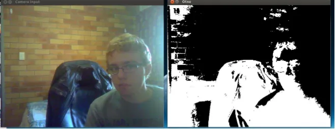
Otsu (Otsu 1979), which suggests that a planar grayscale image can be reduced to a

binary image given a threshold of intensity to classify each pixel. The Otsu

(27)

variance is minimised. (Otsu 1979) These parameters can be calculated iteratively and

a minimisation expectation applied. (Otsu 1979)

To exhaustively minimise the intraclass variance, the weighted sum of variances of the

two classes can be represented according to:

σ2_w(t) =ω1(t)σ21(t) +ω2(t)σ22(t) (2.1)

ωi represents the weight of each mode, separated according to the thresholdt and the

mode variances represented byσ2_i. (Otsu 1979)

As such, the minimisation of the intraclass variance is the equivalent of maximising the

interclass variance:

σ_b2(t) =σ2+σ2_w)(t) =ω1(t)ω2(t)[µ1(t)−µ2(t)]2 (2.2)

The mean of each class is notated asµi. The class probability can be calculated from

examining the histogram according to:

ω1 = Σt₀p(i) (2.3)

The class mean is derived from:

µ1(t) = Σt₀p(i)x(i) (2.4)

Wherex(i) is the center of theithhistogram bin. The other class probability and mean

can be calculated in converse, by utilising the right side of the histogram starting with

bins which are greater thant.

The threshold is determined by way of an exhaustive search minimisation. (Otsu 1979)

(28)

image to be used as a binary mask. Most commonly, the mask is represented by a

[image:28.595.156.486.138.266.2]

binary image - foreground as white, background as black.

Figure 2.1: An example of a segmentation mask calculated using Otsu thresholding

Whilst the Otsu method yields reasonable results, the classification accuracy is not

robust for applications which stipulate that the previous inputs to the system form

the basis of ground truths for following frames. The use of a single frame of reference

is a naive approach to image segmentation as the changes in the scene do not form

a historical basis for segmentation of future frames. This creates difficulty in setting

boundary conditions and thresholds in order to define rules which govern the detection

of events. Additionally, regions of noise are not effectively eliminated as the use of

only a small number of distributions for the entire image does not facilitate adequate

segmentation depth. The utilisation of an iterative model, which places lifetime

con-straints of the input, allows previous inputs be used in determining the classification of

the pixel components. Additionally, by segmenting the image according to the entire

frame, localised image features are able to affect the segmentation as a whole. This was

not considered to be desirable, as anomalies are required to be localised. In order to

localise anomalies, the segmentation model must encompass many sub-models which

segments the image according to local features, not the features of the neighbouring

regions.

The Effect of Locality

With these limitations in mind, it was noted that methods which rely solely upon

the current image did not present a suitable method of segmentation for use with this

(29)

not rely upon absolute or “forced” segmentation was investigated. Clustering-based

methods assign pixel components to distinct clusters for which the distribution can be

modelled through the formulation of fitted distribution. Typical methods involving the

clustering do not assume that the image will always contain foreground. Models which

are mature and correctly configured will allow for greater accuracy.

The use of a mixtures model allows that the distribution of these clusters be modelled

according to a weighted mixture of components which are updated upon each new

sample to form an adaptive threshold for image segmentation. However, in the case

where events are considered local,, the use of a mixture of only a few components for the

entire image yields many of the same issues as the histogram based methods discussed

previously.

A localised method of mixture modelling calls for the image to be divided into a number

of regions. These regions can be as a small as a single pixel, or many encompass many

pixels. Modelling each of the regions as a separate mixture of Gaussian components

allows for local history to be preserved resulting in more accurate and robust

segmen-tation. By defining the local segmentation in terms of the history of local features,

this enables each part of the image to be considered independent from all others. This

enables the model to cope with gradual changes, and changes will not have bearing

upon any other locale.

The Gaussian Mixture Model

The Gaussian Mixture Model (GMM) provides a clustering means of estimating the

background and foreground distributions through a sum of weighted Gaussian

distri-butions. In essence, it provides a parametric probability density function describing

the distribution of pixel values against background and foreground. (Reynolds 2008)

The GMM can be described by the equation:

p(x|λ) =

M

X

i=1

(30)

Where,

• xis a D-dimensional data vector (in this case, an image)

• The mixture weights are represented bywi, wherei= 1, . . . , M

• g(x|µi,Σi) represent the Gaussian component densities. Again, i= 1, . . . , M.

(Reynolds 2008)

The Gaussian component densities are represented by a D-variate Gaussian function.

This function takes the form of:

g(x|µi,Σi) =

exp{−1

2(x−µi) 0_Σ−1

i (x−µi)}

(2π)D/2p

(|Σi|)

(2.6)

Hence,

• µi is the mean vector, representing the mean for each component.

• Σi is the covariance vector

The mixture weights must satisfy the condition that their sum must add to one (i.e.

PM

i=1wi = 1). (Reynolds 2008)

The use of a GMM for background subtraction has been widely discussed. An

imple-mentation of a GMM with fixed parameters only has a limited scope of application

(Stauffer & Grimson 1999). A common application of the GMM, is to model the base

image (the background) and compare the error of incoming images with the established

model according to a fixed threshold across a fixed number of components. (Stauffer

& Grimson 1999). As changes in the background occur (such as a change in the

in-tensity or direction of shadows), a fixed parameter model will accumulate an error and

potentially allow for spurious event indicators (Stauffer & Grimson 1999).

In order for a system to be robust and not rely upon the user to follow a set of

(31)

environment, the system should be able to adapt to it’s surroundings. (Stauffer &

Grimson 1999). Variations of the GMM make use of adaptive parameter settings

(Stauffer & Grimson 1999) (Zivkovic 2004) (Dar-Shyang 2005) to adjust to gradual

scene changes in order to successfully model the background under varying lighting

conditions. Zivkovic (Zivkovic 2004) suggests a recursive method to adaptively select

the appropriate number of Gaussian components for each pixel. This method differs

from more common methods (Stauffer & Grimson 1999) as there is no fixed number

of Gaussian components. This employs the locality principle discussed in the previous

section, as all parts of the image are considered to be independent and uncorrelated.

To explain the implementation of the adaptive GMM in the algorithmic structure

pro-posed by Zivkovic, we assume that the value of a pixel at time t is denoted by x~(t)_,

the pixel classification as foreground or background can be described as (Zivkovic &

van der Heijden 2006):

p(BG|x~(t)₎ p(F G|x~(t)₎ =

p(BG)p(BG|x~(t)₎

p(F G)p(F G|x~(t)₎ (2.7)

Assumptions surrounding the presentation of foreground objects cannot be made as

there is no information regarding how they are be presented, or when they will appear.

This concept is especially important in cases where relevant motion does not occur on

a spatially or temporally consistent basis. As such, a uniform distribution is applied to

the appearance of foreground objects. Thus, the classification decision can be described

as (Zivkovic & van der Heijden 2006):

p(x~(t)_|_BG₎_{> c}

thr (2.8)

cthr is the component threshold value and is described by:

cthr =

p(F G)p(F G|x~(t)₎

p(BG) (2.9)

(32)

The background model,p(BG|x~(t)_{), is estimated according to a training set,}_χ_(Zivkovic

& van der Heijden 2006). In the context of a system which processes data in or near

real-time, the training set refers to a stream of incoming frames (such as from a camera

or pre-recorded sequence). The training set is used to update the estimated model

and in turn to classify pixels as foreground or background. In practice, assumptions

cannot be made about the stability of the captured scene. It is assumed that the

sample inputs are independent, and that adjacent pixels are uncorrelated. (Zivkovic &

van der Heijden 2006). Realistically, consideration must given to the fact that objects

could be removed from the background or placed in the scene to become part of the

background. Thus, to ensure that the model eventually adapts to these changes, the

training set samples must have a limited lifespan. This is performed by discarding

samples which are older than a given interval (Zivkovic & van der Heijden 2006). This

time interval is determined by the adaptation period,T. The learning rate is therefore,

α= 1/T. (Zivkovic & van der Heijden 2006)

If we denote the overall model estimation as, ˆp(~x|χτ, BG+F G), where at time t,χτ =

{x(t), . . . , x(t−T)}, referring to equation 1, anM component GMM can be represented by:

ˆ

p(~x|χτ, BG+F G) = M

X

m=1

wig(~x, ~µm, ~σm2I) (2.10)

Where,

• µ~1, . . . , ~µm are the estimated pixel means

• σ~1, . . . , ~σm are the estimated variances of the Gaussian components

• I is the identity matrix

According to Titterington (Titterington 1984), the model can be updated recursively.

Given a new set of sample data,~x(t), the components weights, pixel means and variances

(33)

wm =wm+α(om(t)−wm) (2.11)

ˆ

µm = ˆµm+om(t)(α/wm)δ~m (2.12)

~

σm2 =σ~m2+om(t)(α/wm)(δ~m τ _~

δm−σ~m2) (2.13)

Where,

~

δm=~x(t)−µ~m (2.14)

In the context of Titterington’s equations,αdenotes an exponentially decaying window

used as a weighting for the data samples. (Titterington 1984) As discussed previously,

the learning rate is defined according to the adaptation period, and thus α in this

context can be assumed to have the same effect.

Theo~mterms represent the ownership of a sample by an existing Gaussian component.

For new samples, this is initialised to 1 for the closest component with the most weight

(i.e largest value of wm). All other components are set to 0. (Zivkovic & van der

Heijden 2006).

To determine the ownership, the squared distance is calculated in terms of the mth

component by (Zivkovic & van der Heijden 2006):

D_m2(~x(t)) = δ~m

τ _~

δm

~ σm2

(2.15)

The definition of close is determined by comparison against an arbitrary threshold.

(Zivkovic & van der Heijden 2006) If a component is not found within the bounds of

such a threshold, it is not considered close. In such cases a new component must be

initialised. The parameters of such a component are initialised according to the model

(34)

2.3 Signal Processing for Wildlife Monitoring 18 • wM+1=α

• µM~+1 =~x(t)

• σM~+1=σ0, whereσ0 is an appropriate value for initial variance.

(Zivkovic & van der Heijden 2006)

If the maximum number of components has been reached, the component with the least

weight (the smallest value ofwm) is discarded.

The number of components can be determined according to the adjusted update

equa-tion (Zivkovic & van der Heijden 2006)

wm =wm+α(om(t)−wm)−αcτ (2.16)

If the GMM is initialised with a single component centred on the first sample, and

new components are added in accordance with the criterion defined by equation 2.11,

the component m is discarded when the weight, wm becomes negative. In essence,

components which are not supported by the incoming data are removed, and

compo-nents which are supported are added. (Zivkovic & van der Heijden 2006). The value

ofcτ is used to discriminate against components which are not supported. For a given

adaptation period, a suitable interval to determine support levels is required.

Assum-ing an adaptation period of T, the level of support required for a component will be

determined against a given value of cτ. This will be an arbitrarily defined threshold

depending upon the level of sensitivity which is required. A smaller value ofcτ dictates

that an entity must be consistently present for a longer interval in order to register as

a valid component. Likewise, larger values of cτ will depreciate the weighting of the

component and cause it to be discarded faster. (Zivkovic & van der Heijden 2006).

The use of the method proposed by (Zivkovic & van der Heijden 2006) ensures that

motion which adheres to some level of periodicity (i.e. breeze causing leaves to move)

or motion which is not deemed to be in the foreground of the image is eliminated

(35)

elements which were previously registered as foreground will eventually be transformed

to a background component as observation time increases. This supports the need for

a locality aware segmentation method.

In much the same manner as the Otsu method, the output matrix can be used to

eliminate pixels which are not of observational interest.

Computational Performance Considerations

The method proposed in (Zivkovic 2004) offers the potential for a high level of

ac-curacy at the cost of a comparatively high computational complexity. On embedded

devices with low computational power, the use of this method could pose a significant

performance threat.

The reliance upon floating point arithmetic must also be taken into consideration. A

hardware floating point unit (FPU) would need to be present on the system, as emulated

floating point calculations will further degrade performance.

Compressive Sensing for Gaussian Mixture Models

The application of compressive sensing to background subtraction (Shen et al. 2012)

offers the potential for a significant performance increase whilst not limiting the

ac-curacy of the model output. The method proposed by (Shen et al. 2012) draws upon

similar concepts to that proposed in (Zivkovic 2004), again by modelling locales as

in-dividual mixtures model. The compressive sensing is applied by modelling each pixel in

terms of compressible vectors. These compressible vectors allow the reconstruction of

a dense vector from the sparse projection vector. By modelling the projection vectors,

the number of Gaussian components is reduced significantly. (Shen et al. 2012)

For compression purposes, let φ equal a ±1 Bernoulli matrix. (Shen et al. 2012) The

probability of the values of the matrix is computed using a symmetric Bernoulli

distri-bution, bounded between ±1. For optimal performance, the matrix must be balanced

(36)

dimensions ofφ will be dependant upon the size of the compressible vectors, and the

number of projections which are to be modelled.

The image need then be divided into N ×N blocks. In order to model each of the

components asM projections, φneeds to be sized accordingly. The recommendations

put forward in (Shen et al. 2012) suggest a suitable value of M and N to be 8, as using

a block size of 64 pixels and modelling to 8 projections allows for an even balance

between performance and accuracy. To form compressible vectors, each of the blocks

is subsequently vectorised to form aN2×1 matrix.

The compression step involves a reduction in the number of components contained

within the modelled block. This is achieved by way of a simple matrix multiplication

between the compressible vector and φ. Note that the same φ is used for all blocks in

the image. Thus, if y is a projection vector, andx is a compressible vector:

y=φ×x (2.17)

y will be an M ×1 projection vector. The projections are then modelled using a

mixture of Gaussian distributions which greatly mimics the way in which it was applied

in (Zivkovic 2004). Given that x is compressible, given a constant value of φ and an

appropriate value of M, it is apparent that the value in y contains almost all of the

same information inx. (Shen et al. 2012) Thus, the projection vectors can be used to

determine which parts of the image are foreground.

The speed increase is achieved by the fact that number of components which are

rep-resented by the mixture of Gaussians is much less. Considering a traditional model,

consisting of three Gaussian components per pixel for a block of 64 pixels. This equates

to 192 Gaussian components. Using compressive sensing, the 64 pixel block is

com-pressed to a 8 projections. At 3 Gaussian components per projection, this equates to a

mere 24 total Gaussian components. The factor of eight reduction offers a great speed

advantage over traditional models. (Shen et al. 2012) The use of synthetic test sets

sug-gests that the addition of the compressive sensing offers a speed increase of 5 - 7 times.

(37)

model to the compressive sensing method, an image of 320×240 passes through the

compressive sensing method in 56.6 ms, as opposed to the previous method in 280.88

ms. (Shen et al. 2012)

GMM Suitability

The Gaussian Mixtures Model presents a potentially suitable method of classifying

locales within the image. Hence, the Gaussian Mixtures Model was recommended as

the image segmentation method for incorporation into the design of the vision system.

The non-compressive and compressive sensing GMM were considered for suitability. It

was necessary to evaluate and compare the performance both techniques. The

method-ology and outcomes surrounding these tests will be discussed in a later section.

2.3.2 Motion Detection Using Optical Flow

The use of a background subtraction technique allows the system to be ignorant of any

parts of the image which are not deemed of observational importance. However those

parts which are deemed to be important must be observed for changes which indicate

an event has occurred.

Optical flow mathematically models the apparent motion of elements within an image,

in terms of relative motion between frames in a sequence of images. In essence, it is a

form of motion detection which aims to model the movements of an image in terms of

motion and velocity vectors. In some cases, this can be used to model and track the

motion of objects within the frame. For the purposes of this system, optical flow will

only be used to detect the presence of objects which are moving, and any information

collected regarding their trajectories will be disregarded. Thus, a method of optical flow

which localises motion to defined features in not suitable. Hence, a method assumes

that the features to be tracked are present in the frame a priori (sparse optical flow) is

not suitable for this application. Dense optical flow estimates the motion of the entire

(38)

The Farneback Method of Optical Flow

The Farneback Method of Optical Flow provides an estimation of dense optical flow

based on polynomial expansion. (Farneback 2003) For the purposes of explanation,

the polynomial which models the pixel neighbourhoods are assumed to be a simple

quadratic. (Farneback 2003) IfAis a symmetric matrix,b is a vector andcis a scalar,

the local signal model can be expressed as:

f(x) =xTAx+bTx+c (2.18)

(Farneback 2003)

By defining two frames, f1(x) and f2(x), f2(x) is able to be represented as a global

displacement doff1(x). (Farneback 2003)

As such:

f2(x) =f1(x+d) (2.19)

Thus,

f2(x) =xTA1x+ (b1+ 2A1d)Tx+dTA1d+bT1 +c1 (2.20)

This can be simplified by equating the polynomial coefficients to incorporate the

pre-vious frame’s coefficients:

A2 =A1 (2.21)

b2 =b1+ 2A1d (2.22)

c2 =dTA1d+bT₁ +c1 (2.23)

(39)

2.4 Chapter Summary 23

The global displacement,dis able to be calculated provided that at least the matrixA1

is non-singular. This observation will hold true for any level of signal dimensionality.

(Farneback 2003) As such:

2A1d= (b1+b2) (2.24)

d= 1

2 ×A

−1

1 (b1+b2) (2.25)

Each of the pixel neighbourhoods is thus tied to a motion constraint between the two

frames. (Farneback 2003) This would be especially useful should motion need to be

predicted, however for this project the use of an optical flow method was investigated

for the purposes of motion detection in relevant parts of the frame. Hence, motion is

present within the frame if motion vector components with a magnitude other than

zero is detected.

In terms of the vision system, the details of the optical flow method itself were not

considered to be important, as there is no need for a high level of accuracy. The

Farneback optical flow method was considered to be adequate and was recommended

for use in the prototype.

2.4

Chapter Summary

In this section, the literature surrounding current wildlife monitoring methods has been

identified. The shortcomings identified in current methods are a prime candidate for

improvement by the development of a suitable vision system. The need for an accurate

and reliable means of data collection can be greatly supplemented by the use of an

embedded system. Such a system must provide a higher level of accuracy in species

counting and tracking, and provide near-real time data return whilst still remaining

cost effective and minimising the impact on habitat and the environment.

The proposed camera system will include the use of a background subtraction method.

The Gaussian Mixtures Model provides an effective means of localised segmentation

(40)

2.4 Chapter Summary 24

(Zivkovic 2004) and (Shen et al. 2012) are to be compared for suitability in terms of

performance and accuracy when utilising an embedded system.

When combined with an optical flow method, motion in the relevant sections of the

image can be detected. This project will investigate the method proposed in (Farneback

(41)

Chapter 3

Methodology

3.1

Chapter Overview

This chapter covers the research and development methodology utilised for the

devel-opment of the vision system and the evaluation of it’s performance. This chapter also

details risks and hazards and suggests suitable mitigation strategies for their

minimi-sation. Any resources which are required for the completion of each of the stages of

development are outlined in this chapter.

3.2

Research and Development Methodology

The research and development methodology contained herein was developed with an

understanding of how the deliverables would be achieved. This led to a logical

break-down of major tasks.

The development of the vision system called for the design and production of an

unsu-pervised and autonomous system which was able to process frames in real time. The

frame process was to be able to distinguish relevant motion from sample frames in

or-der to minimise spurious captures. The recording state was to be determined on a per

(42)

3.2 Research and Development Methodology 26

on an embedded device.

The images recorded by the system were to be stored in static storage and be accessible

remotely. Thus, the project called for the development and implementation of a number

of distinctlayers. These layers formed the basis of the system and encompassed both

hardware and software components.

At the hardware level, the system required a camera to capture the images and a

suitable interface to retrieve the images for processing. The camera was to be connected

to a suitable computer device with suitable support software for resource management,

networking and device control.

The hardware layer was to be supplemented by a software platform which implemented

a retrieval and buffering method. This layer was designed to feed frames from the

camera to the processing software. Finally, the software system was be able to be

“triggered” and store the recorded images in static storage. As such, several distinct

layers were identified:

• Camera control and buffering layer.

• Frame processing and triggering layer.

• Recording and storage layer.

The interactions between the software and the hardware layers can be illustrated by

the block diagram shown in Figure 3.1.

The evaluation of performance and validation of requirements required the definition

of performance metrics and the design of suitable testing methodologies and analysis

strategies. The outcomes of this step formed the recommendations for further

enhance-ments and suggestions of future research.

Due to the modularity of the project, an incremental development methodology was

adopted. This placed an emphasis on “test first” ideals, and encourages a more

mod-ular design with decreased dependencies. The modmod-ularity of the data structures and

(43)

[image:43.595.160.532.77.434.2]

3.3 Task Analysis 27

Figure 3.1: System Block Diagram

3.3

Task Analysis

The project methodology was refined to the following major steps:

• Investigation of suitable target devices (embedded computer) and support

soft-ware and hardsoft-ware.

• Investigation and implementation of possible suitable image processing techniques

and algorithms.

• Design and implementation of a suitable camera control and frame buffering layer.

• Design and implementation of a suitable recording and storage layer.

(44)

• Performance evaluation and recommendations of suitability, improvements and

recommendations of parameters.

• Delivery of a suitable software prototype.

These tasks were identified as milestones for system development and as indicators of

project progress. The following is an analysis of the details of each of the tasks and

identifies any resources which are required for their completion.

3.3.1 Camera Control and Buffering

The vision system required a software layer to control the camera and buffer frames.

The camera control layer must be able to interface with the camera and retrieve

in-coming frames from the internal buffers provided by Video4Linux. The camera control

mechanism was to include a method to set the frame size and desired frame (sample)

rate.

The buffering mechanism involved the development of a thread-safe (producer-consumer)

frame buffer which is self contained and provides suitable methods for adding and

re-trieving frames.

The resources required for this task were:

• Suitable camera

• Working driver and API to control camera and retrieve incoming frames

• An API which provides suitable thread safety mechanisms (condition variables,

mutexes)

3.3.2 Image Processing

The vision system required the implementation and development of suitable image

(45)

the frame buffering mechanism described in the previous section. Incoming frames are

to be processed to determine if relevant motion is occurring. The frame processing

sequence was broken into four steps:

• Frame preprocessing

• Background subtraction

• Postprocessing

• Motion detection

To facilitate event detection, consideration was given to selection of a suitable

sam-pling rate. If the processing sequence is not able to be performed at a suitable speed,

successful segmentation of the background will not occur. An additional concern is the

detection of fast moving objects. A faster sampling rate will increase the chances of

detection of objects moving through the field. As such, the background modelling and

processing stages were to be computed by the Pandaboard at a speed which can be

considered greater than or equal to real time in order to ensure that buffer overflow

does not occur.

This layer was to also provide the means for user configurable parameters which affect

the output of background subtraction and motion detection. This was to be

config-urable by the user and must not require recompilation, as different use scenarios will

require that parameters be set accordingly to ensure optimal segmentation and

detec-tion.

The resources required for this task are:

• A source of input. This could take the form of the camera control and buffering

layer or a synthetic source.

• A library which provides the requisite data types and rudimentary routines for

(46)

3.3.3 Recording and Storage

Upon processing of frames, if an event has been detected the frame sequence is to be

recorded to a file and stored on a static medium for later use. If a suitable Internet

connection is available, these files will be synchronized to a remote server for retrieval.

To avoid large file sizes and facilitate rapid return of data, each file will contain only the

events of a single hour. Thus, this task called for the implementation of suitable output

measures, configuration of storage mediums and the production and modification of

support scripts to facilitate data return.

The resources required for this task include:

• A working buffering mechanism.

• Static storage medium of sufficient size.

• Support scripts to allow synchronisation of recordings to remote machine.

3.3.4 Testing, Evaluation and Benchmarking

To validate the performance of the system it was necessary to define ground truths

which allow a benchmark of performance to be determined. There are several data sets

which are openly available which provide such a benchmark. These test sets will be

used to validate the accuracy of detection and define boundary conditions for detection.

The aim of this task was to validate the algorithm and signal processing techniques.

The software system was also tested to ensure that it is able to operate as a complete,

self supervised system.

The resources required for this task are:

• All working components.

(47)

3.4 Resource Stipulations 31

• Configured test hardware.

The selection of the test sets will be discussed in a later chapter.

3.4

Resource Stipulations

Due to cost factors and limitations of hardware and software availability, the project

requirements stipulated that several key pieces of hardware and software were be used.

3.4.1 Development & Deployment Hardware

A development workstation which is capable of running a similar environment to the

target device is required for ease of development. The GNU/Linux operating system

provides a free (open source) and robust UNIX-like environment whilst targeting many

devices. Such an environment is able to support the necessary tools suitable for use

with this software system.

The Ubuntu Linux distribution (Canonical Ltd. 2012) provides a simple package

man-agement system which allows a wide variety of software packages to be added to the

system easily. Ubuntu also provides precompiled binaries which target a wide variety

of architectures and a large repository of device drivers. The most recent Ubuntu

re-lease (Ubuntu 12.04) is a long-term support rere-lease, meaning that software updates will

be available for five years. Thus, Ubuntu was considered a suitable target operating

system for this project due to the steady development regime and it’s portability.

The use of Ubuntu Linux allowed the selection of standardised hardware for

develop-ment. The development workstation chosen for this project was a Dell Latitude E6410.

For the target device, consideration was given to price, power consumption, size,

soft-ware accessibility and computational performance. As image processing can be a

com-putationally expensive operation, this discounted many embedded devices as they

(48)

target device selected for this project was to also feature an onboard Floating Point

Unit (FPU) in order to ensure sufficient floating point performance capabilities.

Fur-thermore, the target device was to support the standard software environment.

Due to cost limitations, and the availability of hardware, the Pandaboard (Pandaboard

2012) was selected as target device. The features provided by the Pandaboard include:

• Texas Instruments OMAP4430 system-on-chip. This includes a dual-core ARM

Cortex A9 CPU (with FPU).

• 1 gigabyte of RAM.

• 10/100 Ethernet.

• Bluetooth and WiFi connectivity.

• 2 x USB 2.0 ports.

• SD Card slot for operating system and local storage.

[image:48.595.164.464.467.698.2]

• 5W power consumption.

(49)

(Pandaboard 2012)

The Pandaboard is well supported by the Ubuntu operating system. It is of note

that previous versions of Ubuntu do not support the Pandaboard’s onboard FPU,

merely providing emulated floating point computation. This significantly decreases

the floating point performance of the device and would render the Pandaboard an

unsuitable candidate. However, recent changes in the toolchain has led to the migration

to the “armhf” port of Ubuntu (as opposed to the previous “armel” builds which only

provide emulated floating point computation).

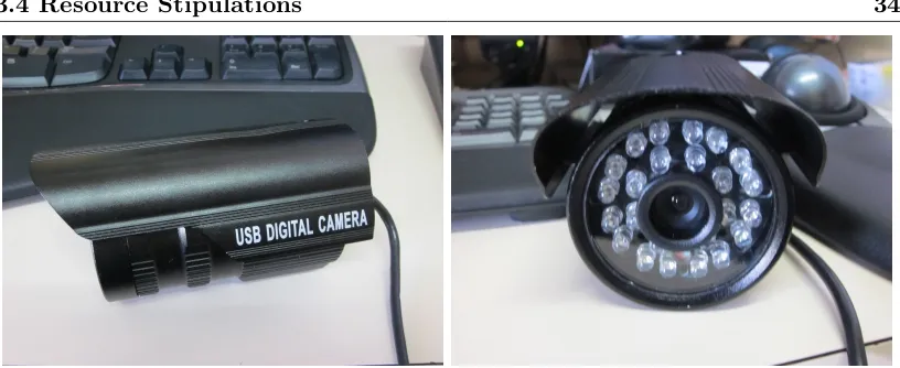
The final hardware component required was a suitable test camera. The camera was

to be weather proof and night vision capable. Due to cost limitations, the camera

selected is generic branded and little information is available. However, the following

specifications are available:

• 640 x 480 maximum resolution.

• 25 frames/sec (maximum).

• Minimum illumination: 0.5 Lux.

• Lens: f = 6mm, F = 2.4 (infrared)

• USB interface providing Y2C video signal.

The Video4Linux API (Linux TV 2011) provides a suitable USB Video Class (UVC)

driver interface to control the camera. This allowed the camera to be compatible with

a wide variety of software packages and libraries.

3.4.2 Software Development Tools

Due to the use of the Linux operating system, an emphasis was placed on the use of

open source software for development. The following software packages were added to

(50)

[image:50.595.117.525.76.243.2]

Figure 3.3: Test Camera

• build-essential- This package provides the GNU Compiler Collection, system

libraries and other development tools such as/usr/bin/make.

• vim- The vim editor (/usr/bin/vim).

• subversion- The Subversion source code management system (specifically,/usr/bin/svn).

The OpenCV Library

The OpenCV (Open Source Computer Vision) library (Bradski 2000) provides data

structures and algorithms for use in real time computer vision applications. Licensed

under the BSD license, the source code is freely available and is able to used as a basis

for building of vision-centred applications.

The OpenCV library provides a number of resources which were applicable to this

application:

• A rich C++ API

• Basic camera control, frame capture and recording classes

• Matrix data types with automatic allocation and deallocation of memory and

type conversion

(51)

• Methods for the creation of rich user interfaces, useful for debugging and data

collection

The OpenCV library is able to be linked to user code at compile time using the GNU

Compiler Collection. The data types and data handling routines provided by OpenCV

will be used as the core vision infrastructure for the system. The addition of specifically

written algorithms and classes will be used to extend the functionality provided by

OpenCV.

The utilisation of the OpenCV C++ API allowed the system to be portable to various

architectures should future requirements change. Many routines provided by OpenCV

include architecture specific performance enhancements, or make use of features

pro-vided by specific system. This was especially important for performance critical work,

whilst retaining portability. The use of a common API allowed the vision system to

be developed and tested on both the development workstation and the Pandaboard

without code changes.

The Boost C++ Libraries

Boost (Boost 2012) provides libraries which are intended to supplement and extend the

capabilities of the C++ programming language, and the standard template library. Of

particular relevance for this project, the Boost libraries provided:

• A runtime arguments parsing and handling library

• A rich threading library, built on POSIX threading paradigms and the provision

of thread synchronization types, such as mutexes and condition variables.

The Ubuntu Linux distribution provides packages which include the relevant

devel-opment files and prebuilt objects for linking with user code. Boost version 1.4.6 was

(52)

GNU Screen

GNU Screen (The GNU Project 2010) is a terminal multiplexer, which allows a console

session to contain many other console sessions. It can also be used to keep sessions

active even if there are no users logged into the system. This was a useful function for

the vision system to ensure that the vision software remains active on the system at all

times, and was selected to be used as part of the self supervision systems.

rsync

rsync (Tridgell, A. and Mackerras, P. 1996) is a network protocol and application

which can be used to synchronise directories and files on multiple machines over a local

network or the Internet whilst minimising the data transferred. Due to bandwidth and

cost considerations, the use of rsync is advantageous to the vision system, as under

deployment conditions the system could be reliant upon Internet connections which

are very costly when transferring large amounts of data.

OpenSSH

The OpenSSH (Secure Shell) protocol (The OpenBSD Project 2012) enables a secure

remote terminal to be opened on the machine via the Internet. This is useful to monitor

and administrate machines which are not local to the user but are able to be accessed

remotely. This was considered to be a useful feature for the vision system, as the

deployment site could be some distance from a convenient place of management.

Python

Python (Python Software Foundation 2012) is a high level, general purpose scripting

language. It supports a wide variety of standard library functions, many of which are

applicable to automation of tasks and machine administration. The Python language

(53)

3.5 Consequential Effects 37

3.4.3 Algorithm Verification Tools

The performance evaluation of the system was designed to demonstrate the suitability

of the signal processing technique

An intelligent vision system for wildlife monitoring

University of Southern Queensland

Certification of Dissertation

Acknowledgments

Contents

List of Figures

List of Tables

Nomenclature

Chapter 1

Project Aim

Project Objectives

Overview of the Dissertation

Chapter 2

Wildlife Monitoring

Signal Processing for Wildlife Monitoring

Chapter Summary

Chapter 3

Research and Development Methodology

Task Analysis

Resource Stipulations