The development of a high precision terrestrial laser scanner calibration range at USQ

(1)

i University of Southern Queensland

Faculty of Engineering and Surveying

The development of a high precision terrestrial laser scanner

calibration range at USQ

A Dissertation Submitted by

Allen Grant Ledger

In fulfilment of the requirements of

Courses ENG4111 and ENG4112 Research Project

Towards the Degree of

Bachelor of Spatial Science (Surveying)

(2)

ii

Abstract

Spatial science firms of today are required to deliver reliable and highly accurate data. Developing technologies have provided spatial science firms with the tools to deliver this data. The latest tool that the spatial scientist can use is the terrestrial laser scanner.

Terrestrial laser scanners are the latest development in the spatial science industry. They are becoming more popular throughout the industry and new applications for their use are constantly being developed. One of the most popular applications is to remotely capture large amounts of data in a short space of time or from locations where it would be dangerous for a human to occupy. For clients to have confidence in the spatial science profession it needs to have a testing procedure that ensures instruments are measuring correctly. It is the purpose of this research project to conduct investigations into developing a calibration range and calibration procedure at the University of Southern Queensland.

There are many design criteria that need to be considered when developing a calibration range. The first major criteria are to have targets located at high and low vertical angles for accurate estimation of the collimation axis error and a vertical angle correction. Having targets in a 360 degree circle around each scanner station is the second design criteria, which is used to calculate a horizontal angle correction. For the calculation of the scale error, multiple distance ranges are required. Finally at least two (2) scanner stations are required to be able to perform the calibration. This project will develop a calibration range at USQ that can be used to estimate corrections to TLS instruments.

(3)

iii

University of Southern Queensland

Faculty of Engineering and Surveying

ENG4111 Research Project Part 1 &

ENG4112 Research Project Part 2

Limitations of Use

The Council of the University of Southern Queensland, its Faculty of Engineering and

Surveying, and the staff of the University of Southern Queensland, do not accept any

responsibility for the truth, accuracy or completeness of material contained within or

associated with this dissertation.

Persons using all or any part of this material do so at their own risk, and not at the risk

of the Council of the University of Southern Queensland, its Faculty of Engineering and

Surveying or the staff of the University of Southern Queensland.

This dissertation reports an educational exercise and has no purpose or validity beyond

this exercise. The sole purpose of the course pair entitled “Research Project” is to

contribute to the overall education within the student's chosen degree program. This

document, the associated hardware, software, drawings, and other material set out in the

associated appendices should not be used for any other purpose: if they are so used, it is

entirely at the risk of the user.

Professor Frank Bullen

Dean

(4)

iv

Certification

I certify that the ideas, designs and experimental work, results, analyses and conclusions set out in this dissertation are entirely my own effort, except where otherwise indicated and

acknowledged.

I further certify that the work is original and has not been previously submitted for assessment in any other course or institution, except where specifically stated.

Student Name: Allen Grant Ledger

Student Number: 0050068403

Signature

(5)

v

Acknowledgements

This research project has been caries out under the principal supervision of Dr. Albert Chong.

I would like to acknowledge and thank all the people who have helped during this research project.

Dr Albert Chong for his guidance and help during the year.

Clinton Caudell for his help and useful advice with the use of the equipment.

Dr Glen Campbell for his help with developing the research question.

Downes Survey Group for the flexible work conditions and their understanding during the year.

(6)

vi

REFERENCES ...58

Appendix A ...60

Project specification ...60

Appendix B ...62

Product specification datasheet ...62

Leica Scan Station 2 ...62

Appendix C ...64

(10)

x

List of Figures

Figure 2.3-1 Principle of time-of-flight

Figure 2.3-2 Calculating phase shift to calculate distance in phased based scanners.

Figure 2.3-3 Leica Scan Station 2

Figure 2.7-1 The HDS target that was scanned and what it looks like in the point cloud

Figure 2.7-2 The Black and White target and what it looks like in the point cloud

Figure 2.7-3 An indoor calibration field

Figure 3.2-1 USQ TLS calibration showing station positions

Figure 3.2-2 USQ TLS calibration showing maximum range

Figure 3.2-3 USQ TLS calibration range showing HDS and BW targets on West wall

Figure 3.2-4 USQ TLS calibration range West wall BW targets only

Figure 3.2-5 USQ TLS calibraation range showing HDS targets only on West wall

Figure 3.2-6 USQ TLS calibration range showing North wall

Figure 3.2-7 USQ TLS calibration range showing South wall

Figure 3.3-1 Screen shot in Cyclone of all the targets in Control space

Figure 3.3-2 Close up screen shot from Cyclone in Control space of the targets

Figure 4.5-1 STN1-STN2 Horizontal residual & CI Limits graph

Figure 4.5-2 STN1-STN2 Vertical residual & CI limits graph

Figure 4.5-3 STN3-STN4 Horizontal residual & CI limits graph

Figure 4.5-4 STN-STN4 Vertical residual & CI limits graph

(11)

xi Figure 4.5-7 STN1-STN4 Horizontal residual & CI limits residual

(12)

xii

List of Tables

Table 2.7-1 Combination of stations

Table 4.3-1 Coordinates from Station 1 and Station 2 of the calibration performed on 26/09/2011

Table 4.3-2 Coordinates from Station 3 and Station 4 of the calibration performed on 26/09/2011

Table 4.4-1 Summary of the results from the calibration performed on the 26/09/2011

(13)

xiii

Glossary

3D: Three dimensional. A description of the spatial environment in reference to its three dimensions.

Co-ordinate system: A set of numerical values that describe the position of a point in three dimensions.

Point Cloud: An array of three dimensional points in space.

Phase Shift: The shift in phase with reference to an electro-magnetic wave.

Total Station: An electronic optical measuring unit used within modern day surveying.

Reflectorless Total Station: A device that measures a distance to an object without the need of

a prism to reflect.

Accuracy: The degree of closeness of a measurement to the true value.

Precision: The degree of repeatability of measurements under unchanged conditions that show

(14)

1

Chapter 1 Introduction

1.1 Outline

This chapter will provide an outline of the project background, research problem, objectives and justification for this project. The dissertation describes the main aspects of Terrestrial Laser Scanner technology and the techniques involved to calibrate terrestrial laser scanner. It covers in detail the mathematical model required to calculate the corrections for the laser scanner. This project seeks to develop a high precision terrestrial laser scanner calibration range at the University of Southern Queensland.

1.2 Introduction

In the spatial science industry of today clients are requiring larger amounts of data faster and more accurately than before. As a response to this spatial science firms are utilising new technology on the market to achieve this.

The latest example of this can be seen with the Global Positioning System (GPS). It was once one of these new technologies that the spatial science industry had to accept and is now commonly used by the spatial science professional in the field. When it was first introduced to spatial science firms many professionals were not aware of it accuracies, errors, what causes those errors and how to manage them. Due to research these questions were answered and confidence was given spatial science firms that use GPS in the field. With this confidence GPS is now a widespread technology and is considered an industry standard in some applications. It would not be widely used if the researchers were not able to identify sources of errors and guarantee the accuracy of its data to clients.

1.3 Project background

Laser scanning is a relatively new technique to the spatial science industry. Spatial science firms are quickly adopting it into their firms. A major reason why these firms are using laser scanners is their ability to capture large amounts of data in a short space of time. This ability allows laser scanners to not only complete conventional tasks but also in ways that were previously thought impossible.

(15)

2 problems could arise if non-professionals are not aware of the measurement errors that could occur. „The increasing application of TLS systems and the ease of data capture they offer have enabled non-specialist operators from outside traditional surveying disciplines to efficiently generate detailed information in evermore challenging and complex environments‟ (Large & Heritage 2009 p.6). This is because they are easy to use and operate and the apparently satisfactorily data outputs.

Calibration of instruments have been used in many different industries not just the spatial science profession. Engineers must have a regular calibration certificate for their measuring instruments. Since the early days of surveying surveyors have had to have a regular calibration policy in their firms. Calibration has been implemented by firms and regulated by the respected spatial science professional bodies of each state. This is because it was required to install confidence in the data given to clients. In Lichti (2009 p.171) „an important aspect of the quality assurance of three dimensional point clouds captured with terrestrial laser scanning (TLS) instruments is geometric calibration. Systematic errors inherent to such instruments can, if not corrected, degrade the accuracy of point clouds captured with a scanner‟.

1.4 The problem

Calibration of measuring instruments has been widely used throughout many industries for many decades. The spatial science profession is no different to any other industry and as such any device that is used should be regularly calibrated. The purpose of calibration is to test the instrument against known values so that corrections can be calculated and then applied to the instrument so that the instrument will measure „true‟. It is difficult to calculate the corrections to TLS because they are built in small series and manufacturers have their own calibration procedure and keep the corrections as a closely guarded secret.

1.5 Project aim

The aim of this project is to develop a terrestrial laser scanner calibration range at the University of Southern Queensland (USQ). That can be used by surveying and engineering firms as a quality control mechanism for their instruments.

1.6 Objectives

(16)

3

 To determine the station geometry for the calibration.

 To determine an optimum target configuration for an outdoor site.

 To determine the capability of the range for TLS calibration.

1.7 Conclusion

(17)

4

Chapter 2 Literature Review

2.1 Introduction

This chapter will outline the relevant literature associated with calibrating terrestrial laser scanners. It will also examine the technology of how terrestrial laser scanners operate. In recent years there has been a sizable amount of research performed on laser scanners. Much of the research has been on the accuracy and precisions of the instruments. There have however been a several researchers who have been successful with the calibration of laser scanners. This review will show and compare the different methods. It will also show the need for calibration of laser scanners

2.2 Need for calibration of Terrestrial Laser Scanners

Terrestrial laser scanning is a relatively new technology in the spatial science profession. It is becoming more popular with firms because new applications for the technology are being thought of. Surveying firms have always had to have a calibration policy for their measuring devices, whether it is an EDM or a steel tape. „The need for calibration is obvious to professionals in those disciplines, it is perhaps more urgent given the significant growth in TLS use, particularly by „non-experts‟ from other fields‟ (Lichti & Jamtsho 2006, p.142).The purpose of calibrating instruments is to define the instrumental errors and provide a correction so that the instrument will measure correctly. Schofield and Breach (2007 p.146) defined calibration as‟ the process of estimating the parameters that need to be applied to correct actual measurements to their true values‟.

(18)

5 Laser scanners are being used where traditional methods would take weeks to gather the minimum amount of data required. In these situations it is not uncommon for the data that is required to be of a very high standard. Laser scanners can achieve these accuracies because of the amount of data that they can gather in a short space of time.

Laser scanners are being used more and more regularly by mining companies to provide the end of month volume calculations. If a spatial science firm does not have a quality assurance (QA) policy for its laser scanners that is similar to EDM calibrations. They could leave themselves open to be challenged by clients. By having QA policy spatial science firms are providing documentation that can be used as evidence to prove that their instrument is measuring correctly. If they do not have a calibrated instrument, clients could argue that the figures that they calculated are in error. For example if the mines earth moving contractor disagreed with the volumes of earth that was moved for that month and believed that they moved more earth than your calculations. You would not be able to argue that your instrument was measuring correctly because you do not having evidence claiming your instrument was correct. This would end up costing the mining company more money because the contractors get paid per cubic meter of earth they move.

Reshetyuk (2009) in his doctoral thesis says that the calibration of terrestrial laser scanners can be performed by one of the following methods.

 Component calibration

The components of the instrument, e.g. laser rangefinder and angle measurement

system, are investigated separately. This type of calibration requires precise knowledge

of the scanner error model. However, this knowledge is often very limited due to

proprietary design of the scanners. In addition, component calibration requires the

access to special facilities, e.g. calibration baselines, which may not be readily

available to the users;  System calibration

System calibration can be performed through what is known in the photogrammetric industry as self-calibration. Self-calibration is the determination of all systematic errors of a terrestrial laser scanner simultaneously with all other system parameters. Unlike in

component calibration, the knowledge of the scanner error model is not very important

in system calibration (or self-calibration). Rather, the error model (or the correction

function) is derived during the calibration, in a least-squares (LS) adjustment (Schulz

2007).

(19)

6

2.3 Terrestrial laser scanner overview

A Terrestrial Laser Scanner (TLS) is essentially a device that measures objects remotely. One of the major advantages of TLS is that you do not need to occupy a space to measure it. This means that delicate or danger areas can be surveyed without putting humans in danger or where they could do damage to a historical site. The basic principle method for this is to calculate a 3D point of the object. TLS do this by measuring a range, horizontal and vertical angle similar to Reflectorless technology in total station instruments. The difference to Reflectorless technology is that a TLS can measure thousands of points per second. Compared to one point for every „shot‟ you take with reflectorless technology. Even though manufacturers are now developing software that can use reflectorless technology in a laser scanner fashion they are still superior for scanning surfaces.

2.3.1 Types of Terrestrial Laser Scanners

(20)

[image:20.595.115.465.56.318.2]

7 Figure 2.3-1: Principle of time-of-flight

„The phase measurement principle compares the difference between the outgoing and the returning signal‟ (Lee & Ehsani, 2008).

Figure 2.3-2: Calculating phase shift to calculate distance in phased based scanners.

[image:20.595.120.406.422.628.2]

(21)

8 Any errors caused by the axes/bearings or angular reading devices will result in errors perpendicular to the propagation path. Since the positions of single points are hard to be verified, few investigations of this problem are known. Errors can be detected by measuring short horizontal and vertical distances between objects (e.g. spheres) which are located at the same distance from the scanner and comparing those to measurements derived from more accurate surveying methods‟ (Boehler & Marbs 2003, p.4).

2.3.2 Accuracy

An investigation into the accuracy of laser scanner has been thoroughly in recent years. Before a calibration can begin an understanding of terrestrial laser scanners is required. This is required so that an appropriate calibration can be designed and procedure developed. Boehler and Marbs (2003) investigating laser scanner accuracy says every point cloud produced by a laser scanner contains a considerable number of points that show gross errors. If the point cloud is delivered

as a result of surveying, a quality guarantee, as possible for other surveying instruments,

methods, and results, cannot be given. If a regular calibration policy is implemented it will help

with assuring clients.

There are many factors that affect accuracy, angular accuracy, range accuracy, influence of surface reflectivity and environmental conditions. Boehler and Marbs (2003) in Investigating

Laser Scanner Accuracy talk about what causes instrumental errors and how to detect these

errors throughout the article.

In Boehler and Marbs (2003) they give a detailed description of how to horizontal and how they occur. . He says that any errors caused by the axes/bearings or angular reading devices will result in errors perpendicular to the propagation path. Since the positions of single points are

hard to be verified, few investigations of this problem are known. Errors can be detected by

measuring short horizontal and vertical distances between objects (e.g. spheres) which are

located at the same distance from the scanner and comparing those to measurements derived

from more accurate surveying methods. This means that the angular accuracy is dependent on

the internal components of the laser scanner.

Ranging errors can be detected when the computed range by the laser scanner is compared to the known distances between two points. If the scanner is not able to be set up over a fixed point then the measured range differences between the targets can be used. Boehler and Marbs (2003) say that „Plane, cylindrical or spherical targets may be used if their precise positions are surveyed with instruments and methods more accurate than the laser scanner‟.

(22)

9 Whereas a systematic scale error will be present in any spatial distance measured, a systematic

constant (zero) error will be eliminated when distance differences in range direction are

determined. The constant error will influence distances between two points which are located

indifferent directions as seen from the scanner, however. If both points are located in the same

distance from the scanner, the deviation of their distance will amount to the zero error when the

direction difference is 60°; it will amount to twice the zero error when the direction difference is

180°.

Boehler and Marbs (2003) believes that this statement is the main reason why a generally acceptable calibration and certification of laser scanners is not possible. Other researchers such as Lichti and Reshetyuk disagree with this statement. They have however in their calibration experiments not rigorously tested for a scale error in the range. This is because in their experiments were conducted in small rooms. Reshetyuk has made an attempt to test for the scale error by using a larger room, but was still not able to test the instrument sufficiently at different ranges.

Laser scanners are an active instrument that is they create a light source that is reflected off an object. „The strength of the returning signals is influenced (among other facts such as distance, atmospheric conditions, incidence angle) by the reflective abilities of the surface‟ (Boehler & Marbs 2003, p.3).

Environmental conditions have been known to affect surveying measuring devices for some time. Therefore they have been studied comprehensively and models to correct for them are being used as a matter of course. Laser scanners operate in a similar fashion to reflectorless technology in total stations, which is why the assumption of using the same corrections for temperature and atmospheric can be used. The temperature correction can only be used if the laser scanner is allowed to warm up internally to a stable temperature. If the laser scanner is not allowed to warm up, then an error called „range drift‟ will occur. Range drift occurs when the temperature changes significantly during the scanning operation. Määttä, Kostamovaara and Myllylä R (1993) say that the temperature of the laser transmitter should be stabilized in order to produce a stable pulse shape. If this is the case, the range drift due to the ambient temperature is linear, and may be compensated for by the software, for example, by reference to frequent temperature measurements‟.

(23)

10 by Lichti (2007) that for planar targets, the signal-to-noise ratio of the measured target centroid drops significantly when the incidence angle is greater than 60 degrees‟. Careful considerations must therefore be given to the location of the laser scanner in relation to the location of the targets.

2.3.3 Applications

The use of terrestrial laser scanners are continuously increasing with spatial science firms realising the possible applications. Some of the areas that are being utilised most are where it requires a person to be put into a dangerous location. Michael Watson from I-SiTE Pty Ltd was‟ commissioned to survey a site a short distance below the Hoover Dam was in the United States of America (USA). To use traditional techniques would have lengthy and hazardous as the banks of the river is cliff like. Aerial surveying was not suitable due to the undercut of the valley faces on either side of the Colorado River. The field work for the whole project took only four days to complete. For the survey the I-SiTE Laser Imaging System was used, which has successfully completed the following applications.

 Excavated areas for volume calculations

 Stockpiles and dumps for volume calculations

 Mining areas for design analysis and geological mapping

 Underground cavities for survey and volume measurement

 Roadways for surface measurement visualisation

 Crime scenes for evidence recording and mapping

 Accident scenes for reconstruction and measurement process

 Industrial plant for measurement, planning and visualisation

 Grain storage facilities for volume calculations

 Disasters areas for scene mapping and recording

 Movie sets and scenery for digital animation and effect creation

 Military and defence applications

 Civil engineering works visual impact evaluation

 Rehabilitation studies in mines

 Vehicle studies for modelling and crash impact evaluation, (photogrammetry and remote sensing 2010, p.278).

(24)

11

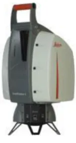
2.3.4 The Leica Scan Station 2

In the last decade terrestrial laser scanning has become more available to spatial science firms. This is because the technology has decreased in price and the benefits are being realised. In the market today there are laser scanners available from many manufacturers. For this research project the Leica Scan Station 2 will be used. It is a pulsed time-of-flight instrument that uses a class 3R green laser. Cyclone software will be used as the operating and processing software.

The manufacture quotes the following accuracies and other important information.

 Modelled surface precision/noise: 2 mm 1 σ

 Scan rate: 50 000 points/second (maximum)

 Maximum sample density: <1 mm

 Field of view: 360˚ horizontal, 270˚ vertical.

 Range300 m @ 90%; 134 m @ 18% albedo

 Dual-axis compensator:Selectable on/off Resolution 1", dynamic range +/- 5'

 Accuracy of single measurement  Position 6mm

 Distance 4mm

 Angle (horizontal/vertical) 60 μrad/60 μrad, one sigma

[image:24.595.290.367.465.609.2]

 Scanning Optics: Single mirror, panoramic, front and upper window design. Environmentally protected by housing and two glass shields

Figure 2.3-3: Leica Scan Station 2

(25)

12

2.4 Other Terrestrial Laser Scanner calibration Research and

Calibration theory

Terrestrial laser scanners have been a recent development in the spatial science industry. As a result the majority of the research has been completed and published since the start of the new century. Investigation into the accuracy of laser scanners has been comprehensively achieved by many researchers. This research has been vital in giving the spatial science industry the confidence in laser scanning technology. Without this confidence the industry would not be able to provide the services to clients.

‘Calibration can be done relatively easily and inexpensively through what is generally called TLS self-calibration‟(Chow et al. 2010). The benefit of this approach is that it can be performed in house and does not need to be sent away to the manufacturer. This is an important advantage because it is very expensive to return equipment to the manufacturer, not to mention the down time of having a very expensive instrument not returning profits.

There have been many researchers that have completed research into the calibration of laser scanners. The most notable amongst these and the most published is Derek D. Lichti from Curtain University of Technology. The paper by Lichti (2007) „Error modelling, calibration and analysis of an AM–CW terrestrial laser scanner system‟ is the most quoted. In this paper he presents a rigorous method for TLS self-calibration using a network of signalised points. The laser scanner that is the focus of the paper is a „phase shift‟ type scanner, the Faro 880. This paper presents a full mathematical model for point based, photogrammetric approach to self-calibration is provided. Lichti (2007) notes that „the focus of this paper is on one particular make and model of amplitude-modulated– continuous-wave (AM–CW) or (phase shift) TLS system, the underlying mathematical models are derived independently of a particular instrument and can therefore be easily modified to suit others‟. Lichti in a number of his publications recognises the similarities between a total station and a TLS and uses these similarities to estimate the corrections that need to be applied to TLS in the calibration.

(26)

13

2.5 Mathematical theory

Terrestrial laser scanners have the same three fundamental axes as total stations, which are the trunnion axis, vertical axis and the collimation axis. It has been found by researchers such as Lichti that physical systematic errors are caused by these three axis‟s not intersecting with each other in a unique point in space. To mathematically describe the systematic errors in TLS systems, the modelling can be performed in a spherical coordinate system. This approach is

adopted here because despite the fact that most TLS systems outputs X, Y, and Z Cartesian

coordinates, the scanner’s raw measurements are horizontal circle readings, vertical circle

readings, and range observations to the object space (Chow et al. 2010).

This approach has been used in photogrammetric calibration for many years and is called the „unified approach to self-calibration‟. In this approach these raw observations are used and compared to each other. For example two targets are scanned from one scanner location. Using laser scanner software the X, Y and Z of the targets are calculated. The horizontal circle readings, vertical circle readings, and range observations can then be calculated between the two targets. A second scan is then performed and the same targets are scanned again. The angles and range are calculated from the second scanner location. The angles and range from each scanner location are compared with each other. The differences between the angles are used to calculate the Additional Parameters (APs) and Exterior Orientation Parameters (EOPs). In a single scan captured by the TLS instrument, every point is uniquely determined. With zero degrees of

freedom, the APs cannot be determined. In order to perform least squares adjustment and solve

for the object space coordinate, exterior orientation parameters (EOPs) of each scan, and APs

simultaneously, multiple scans of the same targets from different positions and orientations

must be captured (Chow et al. 2010).

For the unified approach to self-calibration there must be at least two scanner locations. For the calibration range at USQ we have used three scanner locations. By having three scanner locations there is one degree of freedom and will provide redundancies for the mathematical models.

2.6 Mathematical Models

(27)

14

2.6.1 Simplified procedure

The simplified test procedure was presented at a conference sponsored by Leica and is based on the kick-off document by Hans Heister. The topic was called „ideas for field procedure to test terrestrial laser scanners (TLS)‟. The procedure is valid for all types of scanner, whether they have tilt compensation or not. It does this by appointing common measure of standard uncertainties.

The range error will be calculated as follows (Ideas for field procedure to test Terrestrial Laser

scanners (TLS), 2008).

Therefore

The horizontal error (Hz error) will be calculated as follows (Ideas for field procedure to test

Terrestrial Laser scanners (TLS), 2008).

The vertical error (V error) will be calculated as follows (Ideas for field procedure to test

Terrestrial Laser scanners (TLS), 2008.

These formulas have been used in a Microsoft Excel spreadsheet to estimate corrections.

2.6.2 Point based adjustment

(28)

15

This is a rotational matrix that transforms all of the different scans onto the same datum.

The range, horizontal direction and vertical angle are calculated from the raw uncorrected coordinates of the targets in the scanner (Lichti 2007, p309).

And

The error terms are modelled below (Reshetyuk 2009).

Where is the laser rangefinder zero error (Reshetyuk 2009).

Where and are the collimation and horizontal axis errors, respectively (Reshetyuk 2009).

Where is the vertical circle index error.

(29)

16 instrument. The error model that has been presented are designed for the phase shift TLS that has been used in this project. In Lichti (2007) he has identified 17 error sources for his TLS error models.

The groups of observation equations can be arranged in (linearised) hyper-matrix form as follows (Lichti 2007, p314).

Where represents the Jacobian (design) matrix of partial derivatives of an observation group.

In Lichti (2007) paper inclinometer observations of the targets were made. The two (2) equations for the inclinometer observations have been left out. This is because inclinometer observations would not be made.

The weight matrix P is a block diagonal (Lichti 2007, p314).

(30)

17

Where is the vector of the Lagrange multipliers.

The rigorous mathematical formula requires that targets be coordinated by independent methods. This method will not be used in the reduction process. This is because it was one of the desires of this project that the scanner targets would not have to be coordinated before any scanning was performed.

2.7 Calibration field

(31)

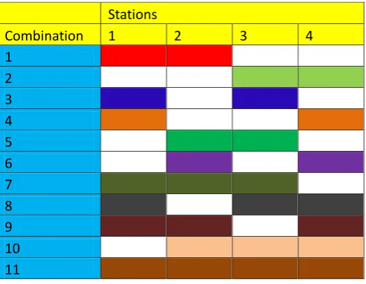
18 The unified approach to self-calibration requires that at least one scan is performed from two locations. Reshetyuk and Lichti both have used four different locations in their calibration fields. They state the reason for this is „a large redundant set of observations needs to be captured with the TLS from multiple positions and different orientations‟ (Chow et al. 2010). By having four scanner stations there is twice the amount of data and are providing the calibration with a complete set of redundant data. It is meant that by a complete set the minimum stations required for a self-calibration is two and by having four you could use to perform many more calibrations with the same data. For example stations 1 and 2 could be used in the calibration but then if you thought that data was corrupted you could use stations 2 and 4. It could be taken further by having stations 1 and 3 in the calibration. A spreadsheet showing all the possible combinations is shown below.

Stations

Combination 1 2 3 4

[image:31.595.110.377.278.485.2]

1 2 3 4 5 6 7 8 9 10 11

Table 2.7-1: Combination of stations

The location of the calibration field that has been chosen for our calibration field is situated on the University of Southern Queensland Toowoomba campus, between the Alison Dickson Centre and the east side of G-Block. An outdoor calibration field has been chosen so that we could simulate a real life scenario, whereas Reshetyuk and Lichti have used indoor calibration fields. They have done this so that all the conditions of the test can be controlled.

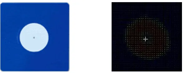
2.7.1 Targets

(32)

[image:32.595.116.416.55.174.2] [image:32.595.124.429.249.419.2]

19

Figure 2.7-1: The HDS target that was scanned and what it looks like in the point cloud

Figure 2.7-1: The Black and White target and what it looks like in the point cloud

2.7.2 Target Configuration

The target configuration design is a very important aspect in the calibration of TLS. The research that has been performed by Lichti and Reshetyuk has based their design on photogrammetric calibration. In Lichti (2007) he notes the following requirements for the design of target configuration.

 A large elevation angle range is needed for estimation of the collimation axis and trunnion axis errors

 At least two locations and a variety of ranges are needed for rangefinder additive constant determination. A large variety of ranges was also needed to estimate cyclic errors.

(33)

[image:33.595.114.491.124.412.2]

20 These points are the same for „First Order Design‟ datum definition in camera self-calibration. Reshetyuk in his doctoral thesis also uses the same principles for his calibration experiments.

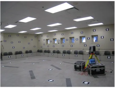
Figure 2.7-1: An indoor calibration field

In the photo above is a calibration field that was used by Lichti (2007) in a series of experiments in 2007. It can be seen that a large number of targets have been used and that they are at high and low vertical angles. Other researchers have used similar sized rooms and placed targets on the ceiling as well.

2.8 Conclusion

(34)

21

Chapter 3 Methodology

3.1 Introduction

The aim of this chapter is to develop and calibration range at the University of Southern Queensland. The desired outcome of the methodology should be the ability to test TLS in a controlled environment where corrections can be calculated and applied with absolute consistency. In order to achieve this, a calibration range and procedure must be developed that compares fixed points with scanned data.

3.2 Calibration design

[image:34.595.116.521.433.721.2]

It was recognised early in the designing of the calibration range that it should be a simple design. It should be as basic as possible while still meeting all the design criteria. For a calibration range to function properly it must also be repeatable. This will allow for the calibration range to be used in the future and ultimately provide a rigorous calibration of the instrument. Finally the test should be able to be used by all the different types of scanners available on the market and any future instruments. In the figures below it can be seen where the target and scanner stations were located.

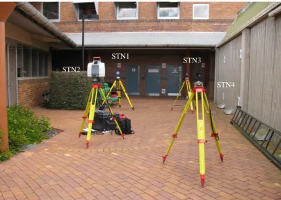
Figure 3.2-1: USQ TLS calibration showing station positions

STN2

STN1

STN3

(35)

[image:35.595.116.524.164.458.2]

22 In figure 3.2-1 shows where the scanner was positioned during the data capture. HDS targets have been placed on these tribrach‟s because they were originally going to be used in the calibration. It was decided not to use these targets because centring errors would be brought into the calibration. Any procedures that could introduce human errors into the calibration should not be used.

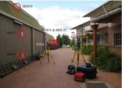
Figure 3.2-2: USQ TLS calibration showing maximum range

In figure 3.2-2 the maximum possible range is shown. It is possible to measure a maximum of 50 meters to the permanent HDS targets located on the far building. The maximum distance could be extended by placing HDS targets on tripods. The tripods would need to be located on the far side of a road and car park that can be seen in the figure.

HDS31 & HDS 32

STN4 STN2

HDS18

BW21

(36)

[image:36.595.114.544.56.621.2]

23

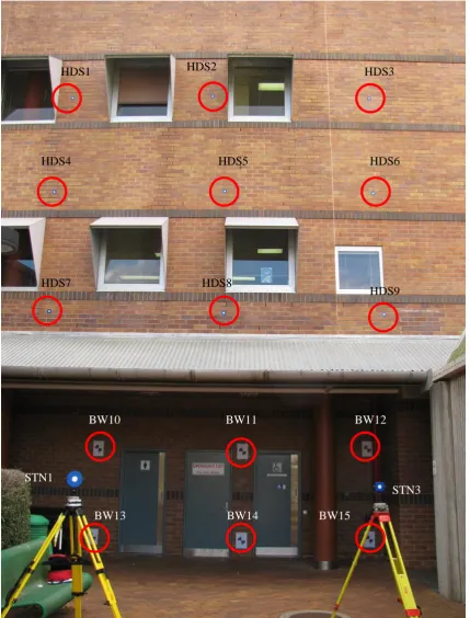
Figure 3.2-3: USQ TLS calibration range showing HDS and BW targets on West wall

In figure 3.2-3 nine (9) HDS and six (6) BW targets have been located on the West wall of the calibration range. The West wall provides for the steepest vertical angle to the targets. All of the scanner stations are located normal to the wall and do not have a large horizontal angle to these targets.

HDS1 HDS2 HDS3

HDS4 HDS5 HDS6

HDS7 HDS8

HDS9

BW10 BW11 BW12

BW13 BW14 BW15

STN1

(37)

[image:37.595.116.498.55.342.2]

24

Figure 3.2-4: USQ TLS calibration range West wall BW targets only

In figure 3.2-4 the BW targets on the West wall can be seen. The targets were fixed to the wall on the day of scanning. They were fixed to the wall using sticky tape.

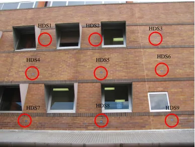
Figure 3.2-5: USQ TLS calibration range showing HDS targets only on West wall

BW10 BW11 BW12

BW13 BW14

BW15

HDS1 HDS2

HDS3

HDS4 HDS5 HDS6

[image:37.595.115.504.438.730.2]

(38)

[image:38.595.113.544.126.448.2]

25 In figure 3.2-5 the HDS targets located on the West wall can be seen. The targets have been located in a grid pattern. The image was taken from between Station 1 and Station 3. These two stations provided for the steepest vertical angles to the targets.

Figure 3.2-6: USQ TLS calibration range showing North wall

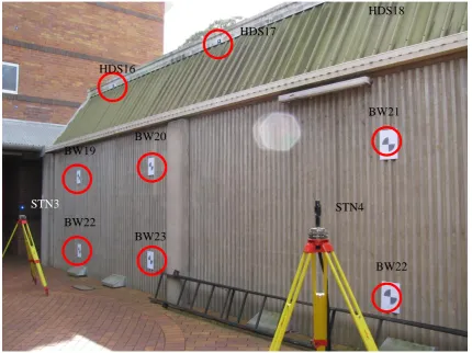
In figure 3.2-6 the location of two (2) HDS target and six (6) BW targets can be seen on the North wall. The temporary BW targets were fixed to the wall on the day of scanning. The wall is concrete with purpose built corrugations in them. Normally a rough surface would not be suitable for the location of a target. To overcome this problem the A4 sheets of paper were glued onto a stiff piece of cardboard and then fastened to the wall using double sided tape. HDS18 cannot be seen in this image as it is out of the shot but is located directly above BW21. The low vertical angle tested because of the closeness of Station 3 and Station 4. These stations also provide a large horizontal angle between the targets because the stations are about one (1) meter from the North wall.

HDS16

HDS17

HDS18

BW19

BW20

BW21

BW22

BW23

BW22

(39)

[image:39.595.114.542.52.377.2]

26

Figure 3.2-7: USQ TLS calibration range showing South wall

In figure 3.2-7 location of the six (6) HDS targets on the South wall can be seen. This wall provides a high vertical angle because of the closeness of Station 1 and Station 2.

3.3 Terrestrial laser scanner

It was mentioned in the literature review that the terrestrial laser scanner that will be used in this project is a Leica Scan Station 2. This instruments operating and functioning software is Cyclone. A Panasonic Tough Book is loaded with Cyclone, which is then used to control the laser scanner in the field.

The Leica Scan Station 2 is terrestrial laser scanner that is capable of filling all the requirements of performing a full calibration. This is because it has a dual axis compensator and has a 360 degree horizontal field of view and more importantly 270 degree vertical field of view. It is important to have a large vertical field of view because it is required to properly estimate the collimation and trunnion axis correction. It was mentioned in the literature review that targets that a larger elevation angle is required for the estimation of the collimation and trunnion axis correction. Some researchers have argued that the compensator should be turned off when scanning the calibration range. They believe that it a better way to estimate the trunnion axis correction. The accuracy of the scanner is not important in the calibration. It will be used

HDS23

HDS24

HDS25

HDS26 HDS27 HDS28

(40)

[image:40.595.116.531.419.579.2]

27 however to determine that the scanner is measuring to the manufacturer‟s specifications. These are quoted for a single measurement of 6mm position and 4mm for distance. For the horizontal and vertical angle is 60 μrad at one sigma.

Figure 3.3-1: Screen shot in Cyclone of all the targets in Control space

In figure 3.3-1 all the targets that were scanned can be seen. This figure is a screenshot of how the targets appeared in Cyclone‟s control space.

Figure 3.3-2: Close up screen shot from Cyclone in Control space of the targets

In figure 3.3-2 a close up screen shot of the targets in Cyclone‟s control space can be seen. The different densities in the scanner can be seen. The fine scans that were used to determine the target centre can be seen in the middle of the course scan data. The course scan data is used to determine the location of the target, where a fine scan can then be used on the target only.

(41)

28 in the field. The scanner and processing equipment was made available by the University of Southern Queensland.

3.4 Calibration

As mentioned in the literature review it was decided to use the unified approach to self-calibration. It was decided that this approach was to be used because it was the simplest method for design and usability. Other methods that require fixed targets to be coordinated by independent methods have problems associated with them. For instance the targets must be „read in‟ with more accurate methods than the laser scanner. As different laser scanners have different accuracies some laser scanners may not be able to be used on the calibration range. Another problem that could arise is if targets are located on buildings or any other structure the coordinated targets could move and would need to be re-observed.

In the unified approach orthogonal scans are performed from different locations. The angles between the targets are calculated from each scanner location. The angles from each scanner location are compared to each other. The angles are compared and adjusted in a rigorous least squares adjustment.

The location of the targets were located that filled the criteria set out in the literature review. They were set up on the outside of different buildings so that they could be seen from different scanner locations.

3.5 Calibration field procedure

The calibration field is located on the outside of Q Blocks east wing at the USQ campus, Toowoomba. This site was chosen because it is not a heavily used area by students. The locations of the scanner station have been located in positions that are not used by students. This location also has the ability of testing the scanner at high vertical angels. This was one of the most important criteria that the range had to pass as it will allow for the trunnion and collimation axis error to be estimated properly. Due to the nature of the location is will allow targets to be placed on both buildings. By doing this it will allow for a wide spread of horizontal angles between the targets. It also allows for varying different ranges for the scanner to be tested at. These ranges vary from about one (1) meter to about 50 meters. It is situated near a road so that it will allow easy transportation of equipment to the site.

(42)

29 calibration. To accommodate this BW targets have been printed out and are temporarily fixed to the walls on the day of scanning. These targets position can be assured for the day of scanning.

Four scanner locations have been chosen to perform that calibration. In the literature review it was shown that at least two scanner locations were needed to perform a calibration. Four have been chosen because it will allow for 2 degrees of freedom on the statistical testing and will therefore provide a better result.

The Leica Scan Station 2 was setup over „station‟ and is levelled and setup properly. As part of the setting up process a „warm-up‟ can must be performed. If this is not the done the range to the targets could be affected by range drift as was seen in the literature review. After the scan is setup, each target can be scanned. For the Leica Scan Station 2 this is done by firstly, the area is imaged using the scanner imagery function. This image is used by the operator to identify the locations of the targets that will need to be scanned with a higher resolution scan. This is a special function of the Leica Scan Station 2 which allows you to select different areas in the scanners field of view that can be scanned at a higher resolution. This speeds up the scanning process because the whole area does not need to be scanned at a high resolution. If a TLS scanner does not have this function then the whole area will need to be scanned at a high resolution. The highest resolution scan should be used in the calibration process. This is because it will allow for the most accurate determination of the targets, which will allow for the best estimation of the corrections that need to be applied to the TLS. This process is repeated for all the scanner locations.

After the field work has been completed the raw data is processed in Cyclone. An arbitrary datum has been used for the coordinates of the scanner stations. An arbitrary datum has been used because we are only comparing the angles between the targets not the actual coordinates of the targets. This raw data is outputted as an X, Y and Z of each target.

3.6 Calibration reduction

The simplified mathematical model that was shown earlier in this literature review was programmed into the Excel spreadsheet. This mathematical model was chosen because it can be easily programmed into the Excel spreadsheet. It is also a self-calibration adjustment whereas the point based mathematical model as the name suggests relies on the targets being coordinated by independent survey methods.

(43)

30 angles and ranges between the targets. The software outputs the corrections that will need to be applied to the TLS, so that it is measuring correctly. The calibration is also an accuracy test this is because that if the correction is less than the manufacturer‟s specifications then the instrument will not need to be adjusted.

3.7-1 Outlier detection and removal

„The observations used in the adjustment can be falsified by gross errors, or outliers, which change the distribution of the observations‟ (Koch 1999. P. 255). It can be very difficult to identify these gross errors but by using statistical analysis on the observations they can be identified. By removing outliers from the adjustment it is ensuring that only data that is a true representation of how the TLS is measuring is used in the adjustment.

It was stated earlier that the simplified mathematical model will be used in the adjustment of the TLS. Another reason that the simplified procedure was chosen for the calibration is that any outliers can easily be identified and removed. This is because a residual is calculated between every target that is used in the adjustment. The main theory behind the simplified procedure is that a distance is calculated between two (2) targets the same distance is calculated between the two (2) targets by using a different formula. It is these distances that are compared against each other and the difference between them is the residual.

To identify the outliers the residuals will be the best indication if any observations are in gross error. For example if the residual was 0.003 or 0.008 and the positional accuracy of the scanner was 0.006 then it could be said that the residual was not in gross error. Whereas if the residual was 1.265 then it could be said that it was in gross error because it is very unrealistic that a TLS would be in such a large error unless the majority of the residuals showed a similar sized error. The best way to see the pattern in the observations is by graphing the residuals for each accuracy test. To show the overall quality of the adjustment the standard deviation of the mean is calculated, which shows how much each observation deviates from the mean. The smaller the standard deviation the more accurate the observations are. The standard deviation is then used to calculate the confidence interval of the observations. It is standard practice in the spatial science industry to use a 95% confidence interval when performing statistical analysis and has been used for this project as well. The upper and lower confidence interval limits have been calculated and also graphed onto the residual graph. This was done to show which of the residuals were outside of the confidence interval limits and to give an indication of the quality of the data.

(44)

31 residuals. The residuals that get removed will be summarised in a table where any possible patterns can be seen.

3.8 Conclusion

(45)

32

Chapter 4 Results

4.1 Introduction

In the methodology chapter, the development of a TLS calibration range and calibration procedure was discussed. A discussion on calibration methods has resulted in a self-calibration approach being adopted, with a further discussion taking place about the design of the target geometry. A calibration range has been designed that will test the accuracy of the laser scanner and be able to estimate corrections that can be applied to the TLS.

The purpose of this chapter is to provide the results of the calibration. Included will be an explanation of what the results show about the instrument. The results presented in this section will show the capability of the calibration range.

4.2 Target location

Before any scanning was completed targets were required to be located in suitable positions. Permanent HDS targets were located at high vertical angles with the use of a cherry picker. On the day of the field work was commenced temporary printable black and white (BW) targets were fixed to the walls at low vertical angles. These targets were printed out on A4 paper and attached to the walls using sticky tape. Six (6) targets were required to be located on an uneven surface where an accurate determination of the targets was impossible. For these targets the A4 sheet of paper was glued to a very stiff piece of cardboard before it was attached to the wall.

4.3 Terrestrial laser scanner

The field procedure was initiated with a course scan. This process involved the scanner being setup at the desired location and selecting the area to be scanned. The result of this scan is a point cloud of the area. This point cloud is used to identify the HDS and BW targets where a fine scan is then completed around only the target area. A fine scan is used to collect high intensity data at the smallest distance between observations. Cyclone, the operating software of the laser scanner uses this high density point cloud to determine the centre of the target.

(46)

33 Coordinates from station 1 Coordinates from station 2

Target X Y Z Target X Y Z

HDS1 -2.9144 4.6639 7.2457 HDS1 2.0337 -11.0496 7.267 HDS2 -0.0776 5.1959 7.2193 HDS2 -0.8489 -10.8111 7.27 HDS3 3.0653 5.7868 7.2523 HDS3 -4.0299 -10.5509 7.2733 HDS4 -3.0736 4.6346 5.1208 HDS4 2.1959 -11.0642 5.1411 HDS5 0.2113 5.2509 5.1213 HDS5 -1.1358 -10.789 5.1422 HDS6 3.0215 5.7809 5.1196 HDS6 -3.987 -10.5571 5.1407 HDS7 -2.9506 4.6651 2.7157 HDS7 2.0677 -11.0597 2.7356

HDS8 0.2322 5.2648 2.7165 HDS8 -1.16 -10.7968 2.7369

HDS9 3.1112 5.8077 2.7183 HDS9 -4.0796 -10.5582 2.7389

BW10 -2.5016 6.2868 0.3008 BW10 1.207 -12.5058 0.321

BW11 0.3142 6.8127 0.3047 BW11 -1.6481 -12.2677 0.325 BW12 2.7382 7.2661 0.3626 BW12 -4.1064 -12.064 0.3833 BW13 -2.5354 6.2798 -1.4125 BW13 1.2413 -12.5068 -1.3922 BW14 0.3129 6.8123 -1.4102 BW14 -1.6467 -12.2679 -1.39 BW15 2.7438 7.2683 -1.3778 BW15 -4.1118 -12.0636 -1.357 HDS16 4.9327 1.6907 2.6232 HDS16 -4.7482 -6.1072 2.6449 HDS17 5.6689 -2.2593 2.6016 HDS17 -4.4132 -2.1024 2.6232 HDS18 6.4854 -6.6168 2.6018 HDS18 -4.0478 2.3159 2.6239

BW19 4.1772 1.6958 0.432 BW19 -4.021 -6.312 0.4535

BW20 4.771 -1.4638 0.4591 BW20 -3.757 -3.1059 0.4807

BW21 5.6058 -5.9981 0.3814 BW21 -3.3624 1.4868 0.4038 BW22 4.1907 1.6071 -1.2214 BW22 -4.0102 -6.2223 -1.2004 BW23 4.7671 -1.4621 -1.1481 BW23 -3.7538 -3.1096 -1.1266 BW24 5.6026 -6.0015 -1.1412 BW24 -3.3584 1.4884 -1.1186 HDS25 -3.4242 -5.4683 4.7848 HDS25 5.2061 -1.4133 4.8055 HDS26 -4.7514 -2.4938 4.7895 HDS26 5.6983 -4.6325 4.8099 HDS27 -7.0261 2.619 4.7923 HDS27 6.5434 -10.1766 4.8269 HDS28 -0.2479 -14.2209 1.0898 HDS28 2.8647 1.9906 0.5217 HDS29 -1.8261 -4.6076 0.492 HDS29 3.4363 -1.8193 0.5136 HDS30 -4.9001 2.3628 0.4931 HDS30 4.5529 -9.3064 0.5107 HDS31 13.139 -37.5764 -0.0467 HDS31 -2.2734 33.9318 -0.0182 HDS32 14.3125 -43.9948 0.1373 HDS32 -1.7071 40.432 0.1657

[image:46.595.112.548.637.780.2]

STN1 0 1 0 STN2 0 1 0

Table 4.3-1: Coordinates from Station 1 and Station 2 of the calibration performed on 26/09/2011

Coordinates from station 3 Coordinates from station 4

Target X Y Z Target X Y Z

HDS1 -2.8524 6.7247 7.2676 HDS1 -1.7949 13.2908 7.2402

HDS2 -0.1009 5.8332 7.2704 HDS2 1.0217 12.6318 7.2433

HDS3 2.9358 4.8511 7.2739 HDS3 4.1297 11.9068 7.2463

HDS4 -3.0067 6.7751 5.1421 HDS4 -1.9523 13.3281 5.1147

HDS5 0.1729 5.7456 5.1429 HDS5 1.302 12.5675 5.1157

HDS6 2.8946 4.8664 5.1406 HDS6 4.0886 11.9191 5.1143

(47)

34

HDS8 0.1966 5.7475 2.737 HDS8 1.3269 12.5717 2.7104

HDS9 2.9841 4.8478 2.7388 HDS9 4.1803 11.9073 2.7124

BW10 -1.7154 7.9533 0.3216 BW10 -0.7623 14.61 0.2946

BW11 1.0093 7.0683 0.3254 BW11 2.0271 13.9552 0.2987

BW12 3.3548 6.3069 0.3835 BW12 4.4282 13.3921 0.3568

BW13 -1.7485 7.9633 -1.3918 BW13 -0.7956 14.6167 -1.4188 BW14 1.0081 7.0692 -1.3895 BW14 2.0261 13.9555 -1.4165

BW15 3.3613 6.3072 -1.357 BW15 4.4343 13.3914 -1.3837

HDS16 2.6167 0.3601 2.6437 HDS16 4.1745 7.3449 2.6165

HDS17 1.3751 -3.4611 2.6227 HDS17 3.269 3.4928 2.5959

HDS18 0.0091 -7.6806 2.6232 HDS18 2.2573 -0.8243 2.5953

BW19 1.9563 0.727 0.4527 BW19 3.4998 7.7193 0.4263

BW20 0.9664 -2.3323 0.4798 BW20 2.7668 4.5821 0.4535

BW21 -0.4688 -6.716 0.4026 BW21 1.7018 0.0969 0.3761

BW22 1.9249 0.6422 -1.2009 BW22 2.7644 4.5879 -1.1542

BW23 0.9634 -2.3299 -1.1278 BW23 1.6968 0.0962 -1.1464 BW24 -0.4742 -6.7168 -1.1203 BW24 3.4751 7.6271 -1.2279 HDS25 -8.1471 -1.9311 4.8052 HDS25 -6.3496 4.2251 4.7784 HDS26 -7.8902 1.3164 4.8094 HDS26 -6.3634 7.4823 4.7831 HDS27 -7.4436 6.8947 4.8125 HDS27 -6.3827 13.0914 4.7976 HDS28 -6.6468 -5.7799 0.5208 HDS28 -4.5326 0.5131 0.4941 HDS29 -6.3308 -1.9392 0.5123 HDS29 -4.5387 4.3678 0.4856 HDS30 -5.6987 5.652 0.5135 HDS30 -4.5398 11.9861 0.4867 HDS31 -8.9512 -38.0495 -0.0213 HDS31 -4.1431 -31.8358 -0.0484 HDS32 -10.9889 -44.2483 0.1618 HDS32 -5.6575 -38.1818 0.1349

[image:47.595.114.545.52.466.2]

STN3 0 1 0 STN4 0 1 0

Table 4.3-2: Coordinates from Station 3 and Station 4 of the calibration performed on 26/09/2011

4.4 Reduction

(48)

[image:48.842.44.818.77.481.2]

35

(49)

36

4.5 Outlier removal

[image:49.595.114.540.233.497.2]

As can be seen in table 4.4-1, the corrections are quite large and are several times larger than the manufacturer‟s specifications of 4mm for range and 6mm for positional accuracy. It is obvious by looking at the residuals that there are several outliers. To remove the outlier‟s horizontal residual, vertical residual and confidence interval graphs were used to identify any erroneous measurements.

Figure 4.5-1: STN1-STN2 Horizontal residual & CI Limits graph

Figure 4.5-1 shows that there are two outliers that will need to be removed, HDS28-HDS29 and HDS28-HDS30 -6 -5.5 -5 -4.5 -4 -3.5 -3 -2.5 -2 -1.5 -1 -0.5 0 0.5 H D S1 -H D S2 H D S2 -H D S3 H D S1 -H D S3 H D S4 -H D S5 H D S5 -H D S6 H D S4 -H D S6 H D S7 -H D S8 H D S8 -H D S9 H D S7 -H D S9 B W 1 0-B W 1 1 B W 1 1 -B W 1 2 B W 1 0 -B W 1 2 B W 1 3 -B W 1 4 B W 14 -B W 15 B W 1 3 -B W 1 5 H D S1 6 -H D S1 7 H D S1 7 -H D S1 8 H D S1 6 -H D S1 8 B W 1 9 -B W 2 0 B W 20 -B W 21 B W 1 9 -B W 2 1 B W 2 2 -B W 2 3 B W 23 -B W 24 B W 2 2 -B W 2 4 H D S2 5 -H D S2 6 H D S2 6 -H D S2 7 H D S2 5 -H D S2 7 H D S2 8 -H D S2 9 H D S2 9 -H D S3 0 H D S2 8 -H D S3 0

STN 1 - STN 2 Horizontal Residual & CI Limits

(50)

[image:50.595.114.541.57.308.2]

37

Figure 4.5-2: STN1-STN2 Vertical residual & CI limits graph

In figure 4.5-2 the outliers that will be removed are HDS7-BW10, HDS9-BW12 and HDS25-HDS28.

Figure 4.5-3: STN3-STN4 Horizontal residual & CI limits graph

In figure 4.5-3 the outliers that will need to be removed are BW22-BW23, BW23-BW24 and BW22-BW24. -4.5 -3.5 -2.5 -1.5 -0.5 0.5 1.5 H D S1 -B W 1 3 H D S1 -H D S4 H D S4 -H D S7 H D S7 -B W 10 BW 1 0-BW 1 3 H D S2 -B W 1 4 H D S2 -H D S5 H D S5 -H D S8 H D S8 -B W 11 BW 1 1-BW 1 4 H D S3 -H D S1 5 H D S3 -H D S6 H D S6 -H D S9 H D S9 -B W 12 BW 1 2-BW 1 5 H D S1 6 -B W 2 3 H D S1 6 -B W 1 9 BW 1 9-BW 2 3 H D S1 7 -B W 2 2 H D S1 7 -B W 2 0 BW 2 0-BW 2 2 H D S1 8 -B W 2 4 H D S1 8 -B W 21 BW 2 1-BW 2 4 H D S2 5 -H D S2 8 H D S2 6 -H D S2 9 H D S2 7 -H D S3 0

STN1 - STN2 Vertical Residual & CI Limits

Residual CI Lower Limit CI Upper Limit

-5 -4 -3 -2 -1 0 1 2 3 H D S1 -H D S2 H D S2 -H D S3 H D S1 -H D S3 H D S4 -H D S5 H D S5 -H D S6 H D S4 -H D S6 H D S7 -H D S8 H D S8 -H D S9 H D S7 -H D S9 B W 1 0 -B W 1 1 B W 1 1 -B W 1 2 B W 1 0 -B W 1 2 B W 1 3 -B W 1 4 B W 1 4 -B W 1 5 B W 1 3 -B W 1 5 H D S1 6 -H D S1 7 H D S1 7-H D S1 8 H D S1 6 -H D S1 8 B W 1 9 -B W 2 0 B W 2 0 -B W 2 1 B W 1 9 -B W 2 1 B W 22 -B W 23 B W 2 3 -B W 2 4 B W 2 2-B W 2 4 H D S2 5 -H D S2 6 H D S2 6 -H D S2 7 H D S2 5 -H D S2 7 H D S2 8 -H D S2 9 H D S2 9 -H D S3 0 H D S2 8 -H D S3 0

STN3 - STN4 Horizontal Residual & CI Limits

[image:50.595.113.542.403.691.2]

(51)

[image:51.595.113.541.58.347.2]

38

Figure 4.5-4: STN-STN4 Vertical residual & CI limits graph

In figure 4.5-4 the outliers that will be removed are HDS7-BW10, HDS9-BW12, HDS25-HDS28, HDS17-BW22, HDS18-BW24 and BW21-BW24.

Figure 4.5-5: STN1-STN3 Horizontal residual & CI limits graph

In figure 4.5-5 the outliers that will need to be removed are HDS29 and HDS28-HDS30. -7 -5 -3 -1 1 3 5 7 H D S1 -B W 1 3 H D S1 -H D S4 H D S4 -H D S7 H D S7 -B W 1 0 B W 1 0 -B W 1 3 H D S2 -B W 1 4 H D S2 -H D S5 H D S5 -H D S8 H D S8 -B W 1 1 B W 1 1 -B W 1 4 H D S3 -H D S1 5 H D S3 -H D S6 H D S6 -H D S9 H D S9 -B W 12 B W 1 2 -B W 1 5 H D S1 6 -B W 2 3 H D S1 6 -B W 1 9 B W 1 9 -B W 2 3 H D S1 7 -B W 2 2 H D S1 7 -B W 2 0 B W 20 -B W 22 H D S1 8 -B W 2 4 H D S1 8 -B W 2 1 B W 2 1 -B W 2 4 H D S2 5 -H D S2 8 H D S2 6 -H D S2 9 H D S2 7 -H D S3 0

STN3 - STN4 Vertical Residual & CI Limits

-6 -5 -4 -3 -2 -1 0 H D S1 -H D S2 H D S2 -H D S3 H D S1 -H D S3 H D S4 -H D S5 H D S5 -H D S6 H D S4 -H D S6 H D S7 -H D S8 H D S8 -H D S9 H D S7 -H D S9 B W 1 0 -B W 1 1 B W 1 1 -B W 1 2 B W 1 0 -B W 1 2 B W 1 3 -B W 1 4 B W 1 4 -B W 1 5 B W 1 3 -B W 1 5 H D S1 6 -H D S1 7 H D S1 7 -H D S1 8 H D S1 6 -H D S1 8 B W 1 9 -B W 2 0 B W 2 0 -B W 2 1 B W 19 -B W 21 B W 2 2 -B W 2 3 B W 2 3 -B W 2 4 B W 2 2 -B W 2 4 H D S2 5 -H D S2 6 H D S2 6 -H D S2 7 H D S2 5 -H D S2 7 H D S2 8 -H D S2 9 H D S2 9 -H D S3 0 H D S2 8 -H D S3 0

STN1 - STN3 Horizontal Residual & CI Limits

[image:51.595.114.540.443.683.2]

(52)

[image:52.595.115.541.53.298.2]

39

Figure 4.5-6: STN1-STN3 Vertical residual & CI limits graph

In figure 4.5-6 the outliers that will be removed are HDS7-BW10, HDS9-BW12 and HDS25-HDS28.

Figure 4.5-7: STN1-STN4 Horizontal residual & CI limits residual

In figure 4.5-7 the outliers that will need to be removed are HDS28-HDS29, HDS28-HDS30, BW22-BW23, BW23-BW24 and BW22-BW24.

-4.5 -3.5 -2.5 -1.5 -0.5 0.5 1.5 H D S1 -B W 13 HD S1 -HD S4 HD S4 -HD S7 H D S7 -B W 1 0 B W 1 0 -B W 1 3 H D S2 -B W 1 4 HD S2 -HD S5 HD S5 -HD S8 H D S8 -B W 11 B W 1 1 -B W 1 4 H D S3 -H D S1 5 HD S3 -HD S6 HD S6 -HD S9 H D S9 -B W 12 B W 1 2 -B W 1 5 HD S1 6-BW 2 3 HD S1 6-BW 1 9 B W 1 9 -B W 2 3 HD S1 7-BW 2 2 HD S1 7-BW 2 0 B W 2 0 -B W 2 2 HD S1 8-BW 2 4 HD S1 8-BW 2 1 B W 2 1 -B W 2 4 H D S2 5 -H D S2 8 H D S2 6 -H D S2 9 H D S2 7 -H D S3 0

STN1 - STN3 Vertical Residual & CI Limits

-6 -5 -4 -3 -2 -1 0 1 2 3 H D S1 -H D S2 H D S2 -H D S3 H D S1 -H D S3 H D S4 -H D S5 H D S5 -H D S6 H D S4 -H D S6 H D S7 -H D S8 H D S8 -H D S9 H D S7 -H D S9 B W 1 0 -B W 1 1 B W 1 1 -B W 1 2 B W 1 0 -B W 1 2 B W 1 3 -B W 1 4 B W 1 4 -B W 1 5 B W 1 3 -B W 1 5 H D S1

The development of a high precision terrestrial laser scanner calibration range at USQ