Adding renewables to the grid: Effects of Storage and Stochastic Forecasting

(1)

Rochester Institute of Technology

RIT Scholar Works

Theses

6-24-2019

Adding renewables to the grid: Effects of Storage

and Stochastic Forecasting

Naga Srujana Goteti

(2)

Adding renewables to the grid: Effects of Storage and

Stochastic Forecasting

by

Naga Srujana Goteti

A DISSERTATION

Submitted in Partial Fulfillment of the Requirements for the Degree of Doctor of Philosophy in

Sustainability

Department of Sustainability

Golisano Institute for Sustainability

Rochester Institute of Technology

June 24, 2019

(3)

Certificate of approval

Golisano Institute for Sustainability Rochester Institute of Technology

Rochester, New York

______________________________________________________________________________

Ph.D. DEGREE DISSERTATION

The Ph.D. Degree Dissertation of Naga Srujana Goteti has been examined and approved by the dissertation committee as satisfactory for the dissertation requirement for the Ph.D. degree in Sustainability.

Dr. Thomas Trabold, Director of Ph.D. program and Department Chair

Dr. Clark Hochgraf, Dissertation External Chairperson

________________________________________________ Dr. Eric Williams, Co-Advisor & Committee Chairperson

________________________________________________ Dr. Eric Hittinger, Co-Advisor, Committee Member

________________________________________________ Dr. Gabrielle Gaustad, Committee Member

(4)

Abstract

The electricity sector contributes to a quarter of global greenhouse emissions, and managing its evolution is a critical sustainability challenge. The context for the development and operation of electricity grids has dramatically changed in recent years. Wind and solar power have become much less expensive. Lower costs combined with increased policy action to address carbon emissions is leading to substantial shares of electricity generated by intermittent renewables. Maintaining a stable electricity supply with intermittency is a critical challenge; storage and natural gas are possible solutions. While policymakers promote storage as green grid technology, low-cost natural gas from hydrofracturing extraction raises the economic hurdle for storage.

Researchers have developed complicated energy system models to help plan grids in the face of the above trends. The research in this dissertation introduces new modeling features that affect the economic and environmental outcomes of the adoption of renewable and storage technologies. First, prior models that explore the future build-out of electricity grids are nearly always deterministic, i.e., they assume that decision-makers have perfect information. Here a stochastic optimization grid expansion model is developed that presumes that expected future fluctuations, e.g. in fuel prices, influence build-out decisions. This stochastic model thus includes uncertainty and risk as core elements: Grid build-out depends on the distribution of system costs. A genetic algorithm with Monte-Carlo simulation is used for co-optimization using two objective functions: “risk-neutral,” which optimizes to minimize average system cost and “risk-averse,” which optimizes to minimize average of the top 5% of costs (also called 95% Conditional Value at Risk (CVaR)). This model is tested for the US Midwest regional grid. The results show that the risk-averse scenario does not increase mean system costs but adds

significantly more wind. These results corroborate prior work showing that electricity system costs can be surprisingly inelastic to renewable adoption and further introduces quantification of how increased renewables lowers cost risk.

(5)

model is developed that accounts for how storage operation would affect prices on the grid and in turn, the operational schedule that yields optimal revenue. Results from modeling the US Midwest region shows that this treatment of storage as a “price maker” affects results. The model indicates that storage increases carbon emissions when it enables a high emissions generator, such as a coal plant, to substitute for a cleaner plant, such as natural gas. In this case, low cost; efficient natural gas generation is relatively better than coal to realize emissions reductions with storage under economic arbitrage until renewables dominate the grid mix.

(6)

Acknowledgements

First and foremost, I am indebted to my Ph.D. advisors Dr. Eric Hittinger and Dr. Eric Williams. Thank you for your continuous support, valuable guidance, and constant encouragement all throughout my Ph.D. journey. On the academic level, you taught me the fundamentals of conducting scientific research and effective communication of the results. Outside the academic world, you helped me with the travel and networking during the conferences, secure fellowship to work at National Renewable Energy Laboratory and participate in other outreach activities. Thanks, Dr. Erics, as I fondly address you both for believing in me and supporting me all throughout my time here. I will look up to you and emulate your research principles as I continue to grow.

My sincere appreciation to Dr. Gabrielle Gaustad for readily agreeing to be part of my committee. Your class on advanced optimization techniques is a backbone to my research work. Thank you for always being there, when I wanted to ask you for career advice, and recommendations. Your valuable insights, constructive feedback, and positivity are treasured.

Thank you to my husband Prathmesh Savargaonkar for pushing me to pursue Ph.D., when I was not sure if this was the path I wanted to take. It has been a roller coaster journey for both of us. I am so proud of your positive attitude towards life, and without you, I wouldn't have reached this point in my life. Thank you for everything and can't wait to start a new journey with you after my Ph.D.

(7)

Dr. Clark Hochgraf, I thank you for readily agreeing to chair my dissertation defense and ensuring that the process is conducted fairly and smoothly.

I acknowledge my funding sources for my research during Ph.D and for my internship at National Renewable Energy Laboratory: The National Science Foundation and the Golisano Institute for Sustainability (GIS). I also would like to express my gratitude to Dr. Thomas Trabold, and Dr. Callie Babbit for their pep talks, career advice, and inspiring me to think as a 'sustainabologist'. A massive shout out to GIS staff- Lisa Dammeyer and Donna Podeszek for all the administrative help and the follow-ups. Lisa Dammeyer, thank you so much for your patience and lending ears to my occasional banters.

Thanks to my internship opportunity at NREL, I acquired immense technical skills much needed in the energy modeling world from my mentor- Dr. Brady Stoll, and manager- Daniel Steinberg.

Finally, all this would not be possible without the support from my friends in GIS and at NREL. A special thanks to Wendy Harmon and Vernon Harmon, William Armington, Ashok Sekar, Sherwyn Millette, Aleena Humayun, Haleh Moghaddasi, Vineet Nair, Neha Chengappa, Matthew Irish, Sarah Awara, Elisabeth Mcclure, Parangat Bhaskar, and many many more.

(8)

Table of Figures

Fig. 1 Framework of methodology for determining the optimized grid build out plan under uncertainty of inputs from 2020-2050 across the Midcontinent Independent System Operation (MISO) region. ... 14

Fig. 2 Fuel prices of coal, natural gas, uranium, and oil considered for the deterministic scenario. ... 17

Fig. 3 Natural gas henry hub spot prices and simulated price scenarios from 2018-2050. ... 20

Fig. 4 Simulated hourly load patterns used for Monte Carlo runs in the model. ... 22

Fig. 5 Distribution of natural gas prices from 2020-2050 used for Monte Carlo runs in the model. ... 23

Fig. 6 Brief illustration of flow of steps in the genetic algorithm. ... 28

Fig. 7 Top-figure represents the Capacity mix from 2020-2050 in a risk-neutral scenario, bottom-figure represents the generation mix from 2020-2050 when mean of the stochastic inputs are considered. ... 32

Fig. 8 Probability distribution of the discounted total cost of electricity service for risk-neutral and deterministic scenarios from 2020-2050. ... 33

(11)

(12)

Fig. 24 Quantity of wind and solar required before storage-induced emissions are negative in MISO in the base-case scenario (at $2.6/MMBtu) and high natural gas price scenario (at

$5/MMBtu). ... 66

Fig. 25 Flowchart of methodology for evaluating percentage change in revenue of the power plants after adding storage. ... 76

Fig. 26 Type of fuels used per MWh of energy delivered from the storage for a sample eGRID region CAMX covering California. ... 79

Fig. 27 Fuel type of net energy used per MWh of energy delivered from the storage. ... 81

Fig. 28 Annual percentage change in profit before and after adding storage as a price-maker in Midcontinent Independent System Operator (MISO) and New York ISO (NYISO) without any retirements. ... 83

Fig. 29 Fuel mix of the retired power plants from adding incremental storage capacities. ... 84

Fig. 30 Annual percentage change in profit before and after adding storage as a price-maker in Midcontinent Independent System Operator (MISO), New York ISO (NYISO), and California ISO (CAISO). ... 86

Fig. 31 Percentage change in profit with and without storage in Midcontinent ISO (MISO) as wind capacity is increased from current 14GW to 70GW. ... 87

Fig. 32 Overview and conclusion of the dissertation. ... 92

Table of Tables

Table 1. Overview of knowledge gaps and the contribution of the dissertation ... 6

Table 2. Summary of the inputs, and data sources used in the stochastic model. ... 15

Table 3. Cost and efficiency characteristics of new generation technologies considered in the study based on EIA’s estimates [13]. ... 16

Table 4. Comparison of all the scenarios and summary of the results. The scenarios include deterministic scenario, risk-neutral scenario, and risk-averse scenario. ... 37

Table 5.Average fuel costs used for electricity production during the years 2015-2016. ... 47

Table 6. Variable O&M costs of technologies considered in this study [72]. ... 47

Table 7. Ramping rates of the electricity generators used in the power plants [39, 76, 77].. ... 49

(13)

Table of Appendix Figures

Fig. S1 Total energy storage capacities of different services offered by storage facilities in the US.. ... 105 Fig. S2 Average Variability of the Wind and Solar Energy across 15 potential sites chosen in the MISO region.. ... 107 Fig. S3 Screenshot of the potential sites of wind energy on the map as seen on the NREL Wind Prospector interface, based on the Eastern Wind Integration Dataset. ... 107 Fig. S4 Change in emissions per delivered electricity from storage with the addition of

wind/solar energy on the grid in the Midcontinent ISO (MISO). ... 108 Fig. S5 Real time coal generation mix taken from CAISO website. ... 110 Fig. S5 Top two figures indicate an annual change in generation before and after adding storage per installed capacity of generation technology, expressed in MWh/MW-year. ... 111 Fig. S6. Difference in dispatch stacks with and without storage, during the hours when storage charges and discharges. ... 112

Table of Appendix Tables

(14)

GLOSSARY OF TERMS

Deregulation Wholesale markets for trading electricity generation. Discharge Releasing energy/electricity into the system from storage.

eGRID The Emissions & Generation Resource Integrated Database by EPA. ISO Independent System Operators, coordinates and monitors the electricity

grid such that supply meets the demand. Marginal generator Plant used to meet the last unit of demand.

MW Unit of power output, e.g. nameplate capacities of the power plants. MWh Unit of energy output.

NGCC Natural Gas Combined Cycle. NGCT Natural Gas Combustion Turbine.

Peaker plant Plants used during the peak demand periods. Plant Retirement Plants not in active operation.

Price Maker System’s operation affects the market prices.

Price Taker System exogenous to the market prices and its operation does not affect the prices.

(15)

Chapter 1: Introduction

1.1 Background

Managing the evolution of the electricity grid is a critical sustainability challenge. As of 2017, electricity contributed to the 28% of total greenhouse gas emissions in the U.S. [1] and to a quarter of global GHG emissions [2]. Electricity production is also economically significant, generating $380 billion in revenue in 2016 in the U.S. [3] and is a backbone of many other industries. Not only is electricity a major carrier of energy, its role in the energy system continues to expand. Electric vehicles (EV) could be on a trajectory to enable electricity to replace much of the demand for liquid fuels, prompting expansion and transformation of the electrical grid.

Like any other infrastructure, the electric grid is long-lived. An average age of the coal power plant, accounting for 30% of annual generation in the U.S. is 40 years [4]. Long life exacerbates lock-in effects: Capital investments, once made, last for decades. Sunk investments crowd out the potential to adopt new technology and indeed, some elements of the grid, such as

photovoltaic panels, batteries and wind energy, are undergoing rapid technological improvement.

Deregulated electricity markets

In addition to the long-life of the electricity infrastructure, the deregulation of the electricity industry has shifted the capital availability and risk preferences of generation companies. As of 2018, eighteen states in the U.S. participate in the deregulated electricity markets [5].

Traditionally, in a vertical integrated structure/regulated markets, utilities controlled the transmission, distribution, and generation of the electricity to the consumers. The utilities

(16)

supply a specific number of megawatt-hours of electricity. Independent System Operators (ISO) like Midcontinent ISO in the Midwest region, or New York ISO in the NYISO, clear the market by selecting the generators with lowest bid till the supply meets the demand. The price of the last resource to offer such that the demand meets the supply decides the wholesale price of the power. In such a market with volatile electricity prices, often coal power plants cannot match with the almost zero marginal prices of the renewables and cannot change output like gas power plants in response to demand.

In recent years, a combination of shale revolution and reduction in the wind/solar costs changed the dynamics of electricity markets, pushing flexible natural gas generation and renewables to the forefront over the usage of coal- with higher emission rates. As of 2015, natural gas generation surpassed coal and contributed to 33% of the total generation, followed by coal at 32%, nuclear at 19%, non-hydro renewables at 8%, and hydro at 6% [7]. Also, realizing the economic and environmental benefits of the renewables, states are revising and introducing Renewable Portfolio Standards (RPS) to achieve a certain percentage of the renewable mix in the overall electricity generation. As of today, twenty-nine states in the U.S. have RPS, and eight states have set some form of renewable energy goals [8].

One of the significant limitations of the wind and solar is that they are variable and do not have a firm (constant) output generation. Natural gas complements the variable generation from the renewables and is easy to turn on and off (ramping), based on the availability of renewable energy. Thus, as the renewables grow in the system, natural gas could become even more reliable as a cheap source of energy during the intermittent hours when the renewable resources are unavailable. Also, the clearing prices set by the gas in the current de-regulated markets drives the revenues of the renewables, further bolstering a stable symbiotic relationship between the gas and the renewables [9].

Energy Information Administration (EIA) projects that the gas will be the leading source of electricity supply and the CO2 emissions will remain unchanged until at least 2050 [10]. The

(17)

Energy storage for renewables

On the other hand, energy storage is gaining traction, too, notably amongst policymakers to support the variable renewable generation. It stores energy when the wind blows and the sun shines and discharges into the grid when there is a demand. Storage can be a chemical battery, flywheel, or pumped hydro systems [11]. While the cost of energy storage, especially Lithium Ion batteries are expensive than a traditional gas plant, there has been a steep drop in the recent years from $800/MWh in 2013 to $200/MWh in 2018 [12]. It is a 75% drop in the costs and can soon compete with the natural gas whose Levelized Cost of Energy (LCoE) is between $30-60/MWh as of 2018 [10]. Since the storage overcomes the limitation of producing and

consuming electricity in the real-time, policymakers are increasingly keen on promoting utility-scale and distributed storage systems enabling the integration of the renewables. As of 2018, some of the major states that passed energy storage target mandates are California [13], Massachusetts [14], Maryland [15], New York [16], and New Jersey [17].

Current challenges

(18)

The challenge with the storage systems is that it is promoted by policy makers to solve the intermittency issues of renewable energy. But, storage in the US is rarely used to prevent curtailment of renewable energy. 88% of the total storage capacity in the US operates for profit maximization in an arbitrage scenario [11]. Deregulated grids feature generators (and

consequently storage) as profit-maximizing agents. A profit-maximizing bulk energy storage system charges during low price/low demand periods and discharges during high price/high demand periods, regardless of the type of generation being used. The effect that this economic dispatch of storage has on grid emissions depends upon generation mix, dispatch order, demand, and storage round-trip efficiency [20]. Thus, the storage may or may not benefit the renewables, depending on the grids it operates, and a comprehensive analysis must be performed for different grid types before incentivizing them.

1.2 Problem Statement, research questions and novel contributions

Current energy models do not consider the future weather and fuel price uncertainties, risk preferences in the deregulated energy markets, and the current economic operation of the storage systems. The results from these models could lead to lock-in investments in natural gas for years to come or significant investments in bulk storage. While both the technologies complement the variable nature of the renewables, does the assumption of promoting storage, or results from deterministic grid expansion models help in the growth of the renewables? The research questions develop to answer these challenges are:

(1) Does stochastic forecasting of the future grid for different risk preferences of the market enable more renewables over cheaper natural gas?

(19)

in the generation mix [4]. Application of the model on a grid heavily dependent on the fossil fuels yields insights into trends towards a more sustainable electrical grid.

(2) Can bulk energy storage compliment renewables and enable environmental benefits to the grid?

In chapter 3, storage model is built to evaluate the carbon implications of storage on the current electric grid and grids, and with expanded wind and solar energy. In the next few years, many states around US are keen to implement policy incentives/mandates for encouraging large storage systems on the electricity grids, hoping that it will support renewable growth and decrease emissions. Thus, chapter 3 explores how does storage affect grid emissions with differing amounts of added renewables, and differing natural gas prices? For this case, the New York ISO (NYISO) and Midcontinent ISO (MISO) regions are modeled. The choice of these two case studies allows us to contrast between grids not dependent and dependent on coal. The two grids studied here are representative of many systems in the US and around the world.

(3) Can bulk energy storage enable profit benefits to the renewables?

In Chapter 4, the model examines if adding storage benefits the profits and generation of the renewable energy power plant operators, especially as compared to cheaper natural gas in the system. This study is conducted in two parts. In the first part, the study

(20)

are modeled. These choices allow us to compare across a spectrum of low, medium, and high renewable energy penetration into the grid.

Table 1. Overview of knowledge gaps and the contribution of the dissertation

Knowledge Gaps Contribution

Impacts of future uncertainty and risk preferences in the deregulated markets on the

integration of renewables,

Effects of adding storage on the integration of renewables

(21)

2 Chapter 2: An alternative structure for integration of uncertainty and risk

aversion into capacity expansion models

Abstract

Current capacity expansion models forecast the grid by deterministic optimization to minimize total system cost. Uncertainty analysis is ex-post, via running scenarios varying input parameters. A capacity expansion model with a built-in uncertainty would enable Monte Carlo analysis and consideration of alternative objective functions, e.g. accounting for cost risk. This paper introduces a proof-of-concept stochastic model that includes uncertainty and risk as core elements. Grid build-out now depends on a distribution of system costs; a genetic algorithm is used for co-optimization. Two objective functions are considered: “risk-neutral”, which optimizes to minimize average system cost and “risk-averse”, which optimizes to minimize average of the top 5% of costs (also called 95% Conditional Value at Risk (CVaR)). This study implements the model for the U.S. Midwest region, accounting for distributions in future electricity demand and fuel prices. Curiously, the risk-averse scenario does not increase mean system cost but adds significantly more wind (~ 20GW) and solar capacity (~15 GW) by 2050 compared to the risk-neutral objective. These results corroborate prior work showing that electricity system costs can be surprisingly inelastic to renewable adoption and adds quantification of how increased renewables lowers cost risk.

2.1 Introduction and Literature Review

(22)

the World Energy Model (WEM) by International Energy Agency [23]. It provides medium-long term energy projections on energy consumption, energy transformation, and energy supply levels across the globe, published annually in the World Energy Outlook. Future uncertainties are treated through three different scenario analyses- new policies scenario, current policies scenario and the sustainable development scenario. Another energy system model at the global scale is the World Energy Projection System (WEPS) Model by Energy Information

Administration (EIA)[24]. Similar to WEM, they also model the demand, transformation, and supply at the region scale across sixteen different regions globally. The future scenarios in this model are developed based on the economic growth trajectories in the different regions. Modeling efforts in the U.S. are mostly centered at government agencies and national

laboratories. The National Energy Modelling System (NEMS), coordinated by EIA, is a complex multi-module model that simulates the entire U.S. energy system, including electricity infrastructure, used as the basis for the Annual Energy Outlook published annually. The NEMS is an economy-wide model that also includes the future supply of natural gas, coal, and oil whose data is used by the other popular models for the future price and load trajectories. Another model is The

Regional Energy Deployment System Model (ReEDS) by National Renewable Energy Laboratory (NREL), which is a capacity expansion model extensively focusing on the future scenarios of the U.S. power system, taking into account the technology innovation impacts, and policy scenarios [25]. The capacity expansion of the power system in the above models is optimized such that the generators and infrastructure are built to minimize the total system cost to meet future demand. The usual capacity expansion model is deterministic: The output is a single set of generators and infrastructure that minimizes discounted system costs when faced with a set of deterministic inputs [23, 24, 26].

What is the purpose of grid capacity expansion models? One might first think these models are intended to give reasonable forecasts of the future grid. A capacity expansion model may turn out to be good forecast, but I argue this is not the main purpose for which they are constructed. If energy system models were intended to good forecasts, this would imply that, as with other forecasts such as weather, model construction would involve retrospective analysis to determine what model and data most accurately “forecast” the past. This is not done in any systematic way in building energy models. There is a small literature that notes dramatic

(23)

is not part of a larger modeling effort to incorporate model structure into retrospective evaluation of forecasting.

The real purpose of a capacity expansion model is to construct a future in which society sensibly builds out the future grid. “Sensibly build” usually is defined as minimal total system cost, though often with constraints built in for other societal objectives such as renewable energy adoption targets or a carbon tax. It may be that the actors involved, and their decision-making processes result in a grid reasonably reflecting minimum total cost to society. In spite of this, energy system modelers can argue that there is value in knowing what choices are good for society aside from issues such as market failures.

Uncertainty, however, significantly complicates what it means for society to sensibly build an electricity grid. The usual deterministic optimization used in capacity expansion assumes

decisions are made assuming perfect information, i.e. parameter values are fixed and there is one grid-build out that minimizes system costs. Many parameters driving electricity system

profitability are, however, highly uncertain, including future fuel prices, technology prices, and policies. A choice that minimizes system costs for baseline values of input parameters may in fact, incur high risk of cost increases. Society knows that drivers of energy systems are uncertain and rightly ought to be concerned about lowering risk. To give an example from the sphere of personal decision making, many consumers prefer new cars over used ones because they are sensibly concerned with the costs if something goes wrong, i.e. the car breaking down.

Decision-making that accounts for uncertainty is mathematically formulated as stochastic optimization. Stochastic optimization treats decision makers as possessing knowledge of

uncertainty. The goal is to find a grid build-out that which optimizes an expected (but not

certain) outcome. Following the idea that sensibly building the energy system should account for risk, capacity expansion models should thus use stochastic optimization.

(24)

problem (a decision as a function of a distribution) as a linear problem by using discrete values for alternative parameter values and creating new optimization variables according to the probabilities of alternate parameter values. Switch takes into account the uncertainty in the renewable power supply and future demand. The model co-optimizes the investment and operational decisions under different scenarios of weather conditions. These weather conditions are generated through sample demand patterns, wind, solar and hydro availability chosen from a sample historical date.

The Tools for Energy Model Optimization and Analysis (TEMOA) model [29] also uses similar stochastic linear programming [30–33] for optimization with uncertainty. In this method, uncertain future outcomes are encoded as possible scenarios in an event tree with an assigned likelihood of occurrence. For example: in the sample region of their study using TEMOA, each combination of high, medium, and low growth rates of coal, oil, and gas were divided into 9 branches in an event tree and were assigned an equal probability of 1/9 to each branch. These branches with their assigned probabilities were solved through linear optimization [29, 32]

Stochastic linear optimization has two major limitations in its application to capacity expansion models. The first is the ‘curse of dimensionality’ [34], i.e. the need to define additional optimization variables for each new uncertain variable leads to an event tree increasing exponentially with the number of uncertain parameters. As a result, the current models limit the number of scenario branches/uncertainties from a tree to eight or have to use high-performance computers [35]. The second limitation is lack of flexibility in exploring different ways society might account for risk. For example, society might choose to aim for minimal mean system cost (from a distribution) or show aversion to high cost scenarios. While these different optimization objectives can in principle be treated with stochastic optimization, it is not a natural framework to do so.

This study develops a stochastic capacity expansion model that does not suffer from the curse of dimensionality (i.e. more uncertain parameters can be treated) and is flexible in allowing

(25)

optimization. Given that there is no general analytic solution to non-linear optimization, its use implies numerical approach as opposed to true optimization. There are many possible numerical techniques for nonlinear optimization, this model uses a genetic algorithm because it is suitable for global optimization problems with complex fitness landscapes [36, 37].To summarize our approach, given an initial test build-out model computes a distribution of system costs based on uncertain input parameters. I select an optimization objective, here the two explored are

distribution mean and Conditional Value at Risk’ (CVaR) 95%, i.e. the average of top 5% of the distribution of system costs. From the initial trial, the genetic algorithm generates a sequence of build-outs designed to converge towards the optimization objective. The final result of a run is the build-out with smallest value of the optimization objective. Given the expected variability in numerical approaches, I follow the common practice of running the algorithm 10 times. The resulting distribution of grid outcomes reflects the uncertainty in numerical optimization.

For this case study, this model covers the Midwest region of the U.S., accounting for distributions in two uncertain variables: electricity demand and natural gas prices. Uncertainty in electricity demand is treated by using historical hourly fluctuations in daily to model future variability. The uncertainty in natural gas prices is treated with a mean reversion model, with historical data informing the mean and fluctuations. Other driving variables such as technology cost are deterministic. Build-out decisions are made by minimizing the total cost of service over a 20-year horizon, constrained by the need to meet current and future load.

While there are uncertain variables other than demand and natural gas prices, I treat only these two with the intent of demonstrating the plausibility of stochastic nonlinear optimization in capacity expansion models. Note that using these two distributions is already beyond the

(26)

emissions requirements, 2) it permits examination of the dynamics of the decision-making process rather than simply choosing an optimal grid mix at a fixed point in the future, and 3) uncertainty is integrated into the core of the model, allowing exploration of issues such as the effect that uncertainty over fuel prices and load has on choice of new generation. These advantages are possible due to the use of a general search algorithm, and a model design that accounts for both uncertainty in many elements and the non-myopic nature of the model enables to see effects of decisions in earlier periods have on decisions in later periods. Also, this

approach does not suffer from the curse of dimensionality for the input distributions, and any number of uncertainties can be considered over the input parameters. In the case study presented in this paper, this study limits the input uncertainties to fuel prices and load, but our model is capable of including other uncertainties such as capital costs, policy constraints, learning rates, emission rates, RPS, etc.

2.2 Method

I use a simplified electricity dispatch model to estimate the total costs of electricity service over a 30-year time horizon (2020-2050), given decisions regarding the construction of new electricity generation in each period. A genetic algorithm optimization is used to search for the generation build-out plans that minimize discounted expected total costs of meeting electricity load [37]. Monte Carlo simulation in the core of the model integrates uncertainty in inputs, such as fuel price, and load.

To further explore the risk aversion as a scenario by itself, the model optimizes for not only minimizing the total cost, but also by minimizing the Conditional Value at Risk (CVaR) in a risk averse scenario. CVAR measures the worst-case costs/tail risk in distribution by taking an average of the extreme tail costs after a chosen cut-off. This technique is commonly used in portfolio optimization of stocks. The cut-off used in this study is 95% which means an average of the worst 5% of the costs gives the CVAR value of the distribution at 95%.

(27)

2.3 Modelling Framework

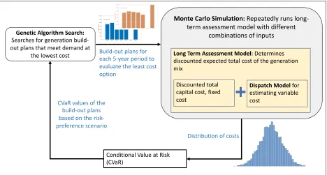
The model has several levels, which interact, as shown in Fig. 1. At the core is a simplified dispatch model that determines whether a set of generation technologies can meet the load and estimates the variable cost of doing so. The long-term assessment model calculates the

discounted expected electricity system costs over a 30-year planning horizon from the fixed costs, capital costs of the new power plants, and the variable costs from the dispatch model. Monte Carlo simulations are performed over the long-term assessment model for a distribution of fuel prices and demand inputs. Given the computational limitations, it is unreasonable to run 30 years of hourly electricity simulation from 2020-2050, considering that the Monte Carlo simulation will perform simulations over the distribution of the inputs. Therefore,

the model operates at 5-year intervals over the 30- year horizon. The output from the Monte-Carlo is a distribution of costs. The distributions are aggregated (like mean) to a single value, based on the risk preference of the markets and given to the decision model. At the highest level, the decision model -genetic algorithm determines the best set of generation technologies to build from 2020-2050. Using this approach allows modification of variables between periods,

(28)

[image:28.612.73.541.71.322.2]

Fig. 1 Framework of methodology for determining the optimized grid build out plan under uncertainty of inputs from 2020-2050 across the Midcontinent Independent System Operation (MISO) region.

The core of the system is the Monte-Carlo simulations of the Long-Term Assessment (LTA) Model, which calculates the distribution of the expected total cost of electricity for different stochastic inputs. Based on a risk preference scenario, Conditional Value at Risk estimates the single point output from the distribution of outputs from the LTA model. Genetic algorithm search is used to identify generation build-out plans that minimize the total

system costs while meeting the future uncertain demand.

2.3.1 Inputs

The inputs to the model can be broadly categorized into stochastic and deterministic inputs. The stochastic inputs to the model are distribution of expected natural gas prices, and distribution of expected electricity demand as a function of season and hour-of-day. The deterministic inputs are expected capital costs, discount rate, technology learning rates, and hourly variations of

wind/solar as summarized in Table 2.

The model is capable of incorporating other uncertainties such as expected future subsidies, distribution of capital costs, RPS constraints, etc. but is not considered in the current study for MISO.

Monte Carlo Simulation: Repeatedly runs long-term assessment model with different

combinations of inputs

Long Term Assessment Model: Determines discounted expected total cost of the generation mix

Discounted total capital cost, fixed cost

Dispatch Model for estimating variable cost

Conditional Value at Risk (CVaR)

Genetic Algorithm Search: Searches for generation build-out plans that meet demand at

the lowest cost Build-out plans for _{each 5-year period to}

evaluate the least cost option

Distribution of costs CVaR values of the

(29)

[image:29.612.72.523.98.384.2]

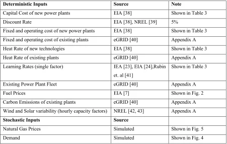
Table 2. Summary of the inputs, and data sources used in the stochastic model.

Deterministic Inputs Source Note

Capital Cost of new power plants EIA [38] Shown in Table 3

Discount Rate EIA [38], NREL [39] 5%

Fixed and operating cost of new power plants EIA [38] Shown in Table 3 Fixed and operating cost of existing plants eGRID [40] Appendix A Heat Rate of new technologies EIA [38] Shown in Table 3

Heat Rate of existing plants eGRID [40] Appendix A

Learning Rates (single factor) IEA [23], EIA [24],Rubin et. al [41]

Shown in Table 3

Existing Power Plant Fleet eGRID [40] Appendix A

Fuel Prices EIA [7] Shown in Fig. 2

Carbon Emissions of existing plants eGRID [40] Appendix A Wind and Solar variability (hourly capacity factors) NREL [42, 43] Appendix A

Stochastic Inputs Source

Natural Gas Prices Simulated Shown in Fig. 5

Demand Simulated Shown in Fig. 4

2.3.1.1 Deterministic Inputs

This section covers about the deterministic inputs used in the model and summarized in Table 2. The model uses the existing portfolio of generation in the studied area, including the age,

efficiencies, emissions, capacities of each plant, to define the starting point for future portfolios from eGRID database [40]. Sample data from the eGRID database is shown in Appendix A.

New Power Plant’s characteristics

New generation technologies and their corresponding capital cost, fixed cost, and efficiencies are considered based on the EIA’s estimates used for modeling the NEMS’ electricity market module [44], shown in Table 3. Overnight capital costs are considered, excluding the

(30)

[image:30.612.63.555.140.353.2]

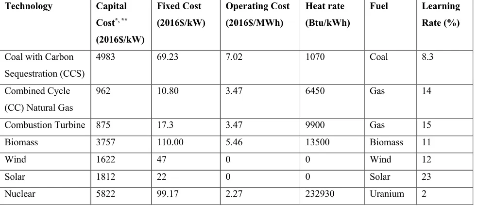
Table 3. Cost and efficiency characteristics of new generation technologies considered in the study based on EIA’s estimates [13].

All the costs are expressed in 2016$. *The capital costs are the overnight costs that exclude interest during the construction and development. ** The capital costs are for the year 2015 and the future capital costs are estimated accounting for the technological progress through learning rates.

Technology Capital

Cost*, ** (2016$/kW)

Fixed Cost (2016$/kW)

Operating Cost (2016$/MWh)

Heat rate (Btu/kWh)

Fuel Learning

Rate (%)

Coal with Carbon Sequestration (CCS)

4983 69.23 7.02 1070 Coal 8.3

Combined Cycle (CC) Natural Gas

962 10.80 3.47 6450 Gas 14

Combustion Turbine 875 17.3 3.47 9900 Gas 15

Biomass 3757 110.00 5.46 13500 Biomass 11

Wind 1622 47 0 0 Wind 12

Solar 1812 22 0 0 Solar 23

Nuclear 5822 99.17 2.27 232930 Uranium 2

Capital costs (accounting for technological progress)

Rapid growth, competition, and technology improvements lead to a significant cost reduction over the time. These cost reductions are generally determined through learning rates. The learning rates (‘LR’) assumed in this study are based on the mean learning rates observed from the literature review by Rubin et.al. in their study [41], given in Table 3.

Learning coefficient a determines the capital cost of the technologies (‘CC’) based on the initial cost (‘CCo’), initial capacity of the technology (‘Po’), and the current cumulative capacity after

the new additions (‘P’) (Eq. 6). Coefficient a is determined from the learning rate of the technologies, which specifies the cost reduction rate, as the technology capacity is doubled

(‘LR’) [45] (Error! Reference source not found.). The total installed capacity of the technology

are determined based on the global level projections from the EIA data [24] and the future capacities in MISO determined by the model.

!" = (1 − 2)) _{Eq. 1}

(31)

--. = --./01

2_. 2_./03

) _{Eq. 3}

Where, Subscript t – given year t LR- Learning Rate

a - Learning Rate coefficient

P – Cumulative capacity (Initial capacity + new capacity additions) P0- Initial Capacity

CC – Capital cost

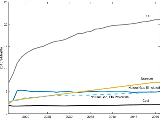
[image:31.612.171.446.321.525.2]

Fuel Prices: Fuel prices of coal, uranium for nuclear power, and oil prices are taken from EIA database [7], shown in Fig. 2, all the units expressed in $/MMBtu for an easy comparison.

Fig. 2 Fuel prices of coal, natural gas, uranium, and oil considered for the deterministic scenario.

The blue dotted line indicates the EIA projection of the natural gas prices. For this study, natural gas prices for the deterministic scenario are estimated from the mean of the stochastic scenario.

Wind/Solar Variability

The hourly generation profiles of solar and wind energy across various locations in MISO are estimated according to the Wind Integration National Database (WIND) toolkit [42] and Eastern Solar Integration Data [43].

2020 2025 2030 2035 2040 2045 2050

Year

0 5 10 15 20 25

2015 $/MmBtu

Coal Oil

Natural Gas Simulated

Natural Gas, EIA Projection

(32)

The WIND Toolkit provides data related to wind energy production for over 126,000 current and potential locations across the United States for 7 years from 2007–2013 [42]. This dataset

consists of meteorological data, 5-min resolution of wind power production, and capacity factors. I consider thirty potential locations in the Midwest region and the corresponding hourly wind output/MW. The average wind energy output (kWh/hour) for a 1kW system across these locations is used to generate the hourly variations of incremental wind capacities considered in the study. Similarly, the Eastern Solar Integration dataset by NREL consist of 5-minute solar power and hourly day-ahead forecasts for approximately 6,000 simulated PV plants. 30 potential sites from 15 states in the Midwest region are considered and a similar procedure to wind energy output is used to generate solar energy output/hour. Annual capacity factors of most of the potential wind power sites in MISO are greater than 40% and most of the solar power sites are greater than 16%. More details on the hourly variation of solar/wind energy output/hour and potential locations considered are provided in the Appendix B section.

2.3.1.2 Stochastic Inputs

In order to model uncertainty, the model will require distributions of possible future values for each input whose uncertainty is considered. In our case, distributions of fuel prices, and load are inputs to the model along with the other deterministic inputs.

Distribution of Natural gas prices:

Volatility in natural gas prices generally exhibit mean reversion and seasonality [46]. Mean reversion is the tendency of natural gas prices to revert to a long-term equilibrium value after fluctuations due to extreme weather, supply, or demand surges. Seasonality is the cyclic

variations over the seasons because of the cyclic changes in demand [46]. In the current model, seasonality of the fuel prices is not considered but only the annual variations using Ornstein-Uhlenbeck (OU) mean-reversion process [47]. Historical variations of the Henry Hub natural gas spot prices since 1986 are used to estimate the future uncertainties.

(33)

Natural logarithm of natural gas prices ptis used in the equation to avoid negative stochastic

prices. Mean reversion rate (a) determines the attraction or repulsive speed from a long-term mean value (µ) of the historical natural gas prices. The volatility (s) is the ‘noise’ in the system based on historical standard deviations of monthly natural gas prices from 1986-2017, obtained from EIA [48]. The annual prices input to the model are an average of monthly prices for a given year. All the historical prices are adjusted to 2016-dollar value.

∆x₆= α(µ − x;<<=<<>₆)∆t

?@AB6

+ σdZG₆

H@IJKALK MI6AIK

, where dZ₆ ~NU0, W∆6X Eq. 4

Where, xt – ln(pt), logarithm of price for a given time t

a - Mean reversion rate

µ- Mean of the log of historical natural gas prices

s- Volatility

N – Random normal distribution

Reversion rate (a), mean (µ) and, volatility (s) are calibrated by dividing the Eq. 5 with Dt and by determining the coefficients of ∆YZ

∆6 based on historical data. Calibration was performed using

‘polyfit’ function in Matlab. The values obtained from the coefficients are a- 0.5022, µ- 1.5030, and s- 0.3963. The solution for the Stochastic Differential Equation in Eq. 4 is as given in the Eq. 5 which is used to generate random time-series of natural gas prices from 2020-2050. A sample of the simulated time series is as shown in Fig. 3.

x6[0 = x6e/∝ + µU1 − e/]^X + σ_0/` ab∝

c] N(0,1)

Eq. 5

(34)

Fig. 3 Natural gas henry hub spot prices and simulated price scenarios from 2018-2050.

Ornstein-Uhlenbeck (OU) mean-reversion process is used to create stochastic natural gas prices as an input to the Long-Term Assessment Model.

Input Demand: Similar to natural gas, demand also exhibits two distinct characteristics –long-term demand growth and the seasonality.

Long term demand growth:

The demand growth is estimated using a simple Brownian motion equation as shown in Eq. 6. The ‘a’ coefficient of the deterministic part in (Eq. 6) is calibrated for a growth rate of 1% every year based on MISO forecast [49]. The σ is the volatility calculated based on the standard deviation of the change in the historical data which is 415.6 MWh from 2007-2017.

L_6[0= L;<₆<=<+ a∆t<>

f`6`@MAKAg6Ah

+ σdZG₆

fABBigAIK

, where dZ₆ ~NU0, W∆6X Eq. 6

Where, Lt- Average load for a given year t

a – Linear coefficient of first order linear equation σ- Volatility

Seasonality and hourly variations:

Seasonality and the hourly variation of the demand are based on the historical load patterns observed in MISO [49]. Percentage change in the load over 8760 hours in a year with respect to

1990 2000 2010 2020 2030 2040 2050

Year 1

2 3 4 5 6 7 8 9 10 11

2015 $/MmBtu

(35)

the mean load for a given historical year is estimated. These percentage changes provide the information on how the hourly load historically varied with respect to the mean demand in a given year. From Eq. 6, a random mean demand value for a year is estimated. Then a historical sample year ‘s’ is chosen with 8760 hourly values of percentage change with respect to the mean demand in that sample year. The new hourly variations are estimated by multiplying the

historical variation (‘V’) with the random mean demand (‘L’) (Eq. 7).

j_k,.,l= !_.∗no,p

0qq Eq. 7

Where, Lt- Average load for a given year t

s- historical sample year h – hour

V- percentage change with respect to mean demand for a sample year s l – hourly load value

Stochastic distributions

(36)

[image:36.612.76.534.81.378.2]

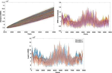
Fig. 4 Simulated hourly load patterns used for Monte Carlo runs in the model.

Top-left figure shows the distribution of average annual load growth from 2015-2050. Each color indicates the stochastic load forecasts from 2020-2050. Top-right figure shows the samples of historical normalized hourly load patterns seen in MISO since 2013. Each color represents the sample of historically observed hourly load patterns in

MISO. The bottom most figure shows two random samples of hourly load patterns in the year 2020. They are created from multiplying a random sample point in the distribution from the year 2020 in the top-left figure with a

random normalized hourly load pattern for an year in the top-right figure. Similar patterns were created at 5-year steps from 2020-2050.

(37)

Fig. 5 Distribution of natural gas prices from 2020-2050 used for Monte Carlo runs in the model. Each color indicates the possible price forecast from 2020-2050.

2.3.2 Dispatch Model for variable costs

The lowest level of the proposed optimization model is a dispatch routine that uses simplified rules to determine the variable cost of electricity generation over a year [25]. Due to the need to run many scenarios, both for the Monte Carlo simulation and the genetic algorithm search, there are limitations on computational time. Therefore, the dispatch model is limited to choosing the generation in each hour based on the marginal cost of operation for 8760 hours in a year.

More sophisticated electricity system elements, such as transmission constraints, ramp limits, startup time and spinning reserves, are not included. However, with a high computational ability, modular nature of the model allows a replacement with sophisticated dispatch models, without major changes to the modeling framework.

The principle of the model is to sequentially add plants to the generation mix in order of the marginal cost (‘MC’) until the demand is met. The output generation (‘e’) of each power plant in a given hour is the capacity of the power plants used to meet the demand. The total variable cost

(‘VC’) of the electricity generation is the marginal cost (‘MC’) incurred by the power plants to

(38)

The current fleet of power plants for electricity generation are taken from EPA's eGRID database [40], and the new generation fleet is added based on the inputs from the decision model and the plant characteristics from EIA data (Table 2) [38]. The marginal cost (assumed as bid price) of operation for each power plant is calculated based on the heat rate [40], and the subsequent fuel costs as given in Eq. 8.

MC_t,.,u v $

MWhy = HR|∗

PriceA,6,B

1000 + O&M|

Eq. 8

VCA,6= É Ñ-t,.,u∗ Öu,.,t,k u,k,.

Eq. 9

Where, Subscript t – hours in a given year Subscript i- ith_{Monte-Carlo run}

Subscript p – Power Plant

e – Energy output in hour t (MWh/h)

MC- marginal cost of operation of a power plant ($/MWh), HR- hear rate (Btu/kWh)

Price- average spot price of fuel ($/MMBtu)

O&M – Operations and maintenance cost of the power plant ($/MWh) VC – Total Variable cost

This study does not model imports of electricity from regions outside of MISO and penalize the model with a high cost of $ 5,000/MWh, when the demand is not met.

2.3.3 Long Term Assessment Model

The long-term assessment model calculates a distribution of discounted expected total system costs (Eq. 10) for meeting load over a 30-year horizon.

Total system cost ($) = Capital cost + Fixed cost + Variable cost TC_A,6= --_.+ é-_.+ è-_t,.

(39)

Where, Subscript t – Given year Subscript i- ith_{Monte-Carlo run}

CC – Capital cost ($) FC – Fixed cost ($)

VC – Total Variable cost ($)

The model operates in 5-year intervals, reducing the model calculations over the 30- year horizon to seven periods. When combined with data on capital and operating costs, the

discounted expected total cost of electricity service over the 30-year horizon is calculated. The start year is 2015 and the costs of other years are extrapolated based on the costs estimated at 5-year intervals.

Cashflow

I assume a discount rate (r) of 5% and calculate costs in the 2016-dollar value as shown in Eq. 11 for a given future value (fv) in the year t.

C_A = ∑ ëíì,Z (0[@)(Zaî) cqïq

6ñcq0ó Eq. 11

Where, Subscript i- ith_{Monte-Carlo run}

C- Discounted present value of the cost TC – Total cost

r-Discount rate, 5% t-for a given year Y- reference year, 2016

2.3.4 Monte Carlo Simulation

To include the effects of uncertainty in the Long-Term Assessment (LTA) Model, I use Monte-Carlo simulations by running the Long-Term Assessment model iteratively for random

(40)

A total of 20 Monte-Carlo runs are performed for each iteration. Because the process is computationally intensive, the LTA model is not subjected to larger number of Monte Carlo runs. However, the genetic algorithm is an iterative process, it identifies an optimized build-out plan, each time subjected to a distribution of the inputs, and identifies a build-out plan that consistently has the lowest discounted cost of the electricity service. The number of iterations of the genetic algorithm are around 800 before the model converges to a solution.

Deterministic scenario is run using the mean natural gas prices and demand growth and the number of Monte Carlo runs is set to 1 in the model.

2.3.5 Conditional Value at Risk (CVaR)

The output from Monte Carlo simulation is a distribution of output costs for various build-out plans. The cost for optimization to the genetic algorithm in the decision model is calculated based on the CVaR scenario. Risk preference of the model is set at this phase. For a risk neutral scenario, CVaR is 0% and thus, mean of the distribution is fed into the decision model, and for a risk-averse scenario, CVaR is 95% and thus, mean of the worst 5% values are fed into the decision model for optimization (Eq. 12).

DC_íôLö ($) =

∑õ_(úùûü†° íì ¢££ ∗õ)

Eq. 12

Where, C- Total discounted present value of the cost Subscript i- ith_{Monte-Carlo run}

Subscript n – total Monte-Carlo runs

2.3.6 Decision Model -Genetic algorithm for optimization

The decision model uses the genetic algorithm optimization to minimize the cost output from the CvaR, based on the risk preference.

Genetic Algorithm Search:Genetic algorithm is good at rapidly identifying a set of reasonably fit solutions using a heuristic optimization algorithm derived from natural selection process. The genetic algorithm iteratively modifies a population of individual solutions, in our case,

(41)

selected from the current population as parents to produce children/new build-out plans for the next step/generation. Fitter individuals/lower cost grid build-out plans have a higher probability of getting chosen as parents. The children are created using different crossover techniques, and over time, the population ‘evolves’ towards an optimal solution [50].

The algorithm broadly works on four essential rules: 1) evaluation, 2) selections rule, 3) crossover rule, and 4) mutation. Evaluation rule applies to calculating the cost of the build-out plans after each iteration in the genetic algorithm. Selection rule applies to assigning

probabilities and choosing individuals/generation build-out plans for creating children/new-grid build-out plans. Probability scores to each individual are assigned based on their fitness/expected total cost. Lower the cost (output from CVaR), higher the probability of becoming a parent for the next generation. Crossover rule applies to the process of creating children/new build-out plans from the chosen parents. These children replace weaker individuals with a high cost. In order to avoid local optimization, mutation rule is applied to create ‘genetic diversity’ in the pool. Based on a user-defined mutation probability, a random bit in the child chromosome/binary form of the new generation build-out is altered before re-converting the children to decimal forms. In our case, the probability of a mutation is set to 3%. The model uses global

(42)

[image:42.612.137.479.72.292.2]

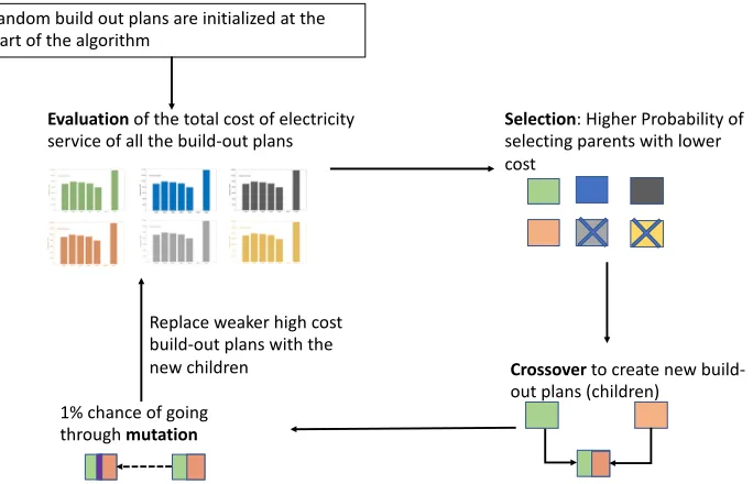
Fig. 6 Brief illustration of flow of steps in the genetic algorithm.

The four principles of genetic algorithm are 1) evaluation of discounted total cost of the build-out plans based on a risk-preference scenario, 2) selection of parents for creating next generation of build-out plans, 3) crossover of parents to create children, and 4) random mutation to avoid local optimization. These steps are repeated till the

change in total cost of electricity service remains constant within the set tolerance levels.

2.3.7 Objective function and summary of equations:

The total cost (‘TC’) for a given year in a given Monte-Carlo run (‘i’) is estimated from the marginal cost of operation from the dispatch model, fixed cost, and capital cost of new power plants (Eq. 15). Maximum electricity generated by a power plant in an hour ‘T’ does not exceed the name plate capacity (‘P’) of the power plant, shown in equation (Eq. 18). Name plate capacity also includes an additional large capacity of 1000 GW at a high penalty cost of $5,000/MWh, in case the new power plants from the genetic algorithm fail to meet the total demand (‘L’). This is to ensure that the total generation always meets the demand which varies for each Monte-Carlo run (Eq. 16). All the total costs (‘TC’) for a given year ‘t’ are adjusted to the reference year 2016 dollar value to evaluate the total net present value of the cost (‘C’) (Eq. 14). In the final step, Eq. 13 shows the objective function of minimizing total discounted electricity service cost (‘DC’) depending on the CVaR scenario.

Objective function, minimize:

DC_íôLö ($) =

∑õ íì

(úùûü†°_{¢££ ∗õ)}

Eq. 13

Selection: Higher Probability of selecting parents with lower cost

Evaluationof the total cost of electricity

service of all the build-out plans

Crossover to create new build-out plans (children)

1% chance of going through mutation

Random build out plans are initialized at the start of the algorithm

(43)

Subject to:

-t = É

TC_A,6 (1 + r)(6/≤) cqïq

6ñcq0ó

Eq. 14

≥-_t,. = ∑¥µ∂q (MC_t,.,k,u∗ e_t,.,k,u )

|,∑ñ0 + ∑ (é-u t,.,u∗ 2u+ --t,.,uõ∏π∗ 2uõ∏π) Eq. 15

É e_A,6,∑,|

ë,|

≥ L_A,6 Eq. 16

e_6,ë,| > 0 Eq. 17

e_6,ë| ≤ 2_. Eq. 18

1 ≤ T ≤ 8760 Eq. 19

Where, C- Discounted present value of the cost,

DC – Discounted cost of electricity service for a given CVaR scenario TC – Total cost of electricity service

i- ith_{Monte-Carlo run}

n – total Monte-Carlo runs r-Discount rate, 5% t-for a given year Y- reference year, 2016 h- hours in a given year Subscript p - Power plant, pnew- new power plants (MW),

MC- marginal cost of operation of power plant ($/MWh) e– electricity generated by power plant in a given hour (MWh) FC- Fixed cost ($/MW)

CC- Capital cost ($/MW)

P – name plate capacity of the power plants (MW) Lt - load (MWh).

Retirement

(44)

regulations [52]. In 2017, most of the retirement decisions in MISO were from uneconomic power plant units [53].

In the current study, economy of the power plants is based on their cost of operation for every 5-year period. The model endogenously retires the power plants by allowing the optimization to randomly choose positive or negative capacity additions. Positive additions denote new generation technologies, and ‘negative’ additions denote retirement of the power plants for a specific fuel type. For the negative capacities, power plants with a high annual cost of operation per unit nameplate capacity for a given fuel type are assumed to be uneconomical to operate and are retired until the retired capacities equal the negative capacities by the genetic algorithm. The total cost of electricity service is then calculated for the resultant build-out.

2.3.8 Reporting output distributions of cost and emissions

The output cost and emissions distributions of the resultant build-outs for different risk

preferences are presented in the section 2.4 below. These distributions are plotted to understand the probability distributions of NPV for deterministic, risk-averse, and risk neutral scenarios.

These distributions are calculated by running the resultant build-outs for different risk

preferences through LTA model and Monte Carlo model. A fixed sample distribution of natural gas prices and demand is assumed for all the build-outs and when run through 1000 Monte Carlo simulations provides a distribution of output costs and emissions. A fixed sample of 1000

different natural gas prices and demand growth patterns is used to ensure a fair comparison between scenarios.

The total annual CO2eq. emissions (in million metric tonnes) for each Monte Carlo run are

calculated based on the hourly dispatch of plants as shown in equations (19-20). The plant-level emission rates are in metric tonnes/MWh, taken from the eGRID database [40] and the emission characteristics of the new power plants are based on the EIA data [38]. Total CO2eq. emissions

(45)

The total CO2eq emissions in a given hour for a given operation schedule of generator plants is

given by Eq. 46:

Subscript i- ith_{Monte-Carlo run}

Subscript p – Power Plant

e – Energy output in hour t (MWh/h)

m – CO2 eq. emissions of plant p per MWh (in metric tonnes/MWh)

em – total emissions (metric tonnes)

2.4 Results

I run an alternative structure for capacity expansion modeling in MISO with uncertainty considered for inputs load and natural gas prices to show comparisons between Deterministic scenario and stochastic scenario; and to compare between risk-neutral and risk-averse scenarios when the inputs are stochastic. The risk-neutral scenario optimizes for the mean of the

distribution, i.e., CVaR at 0, and risk-averse scenario optimizes for CVaR at 95%.

2.4.1 Risk-Neutral Scenario

The base-case scenario is the risk-neutral scenario that optimizes for the mean of the distribution. Output results for MISO show a dominant mix of wind and natural gas in the total capacity by 2050. Though natural gas and coal dominate more than 50% of the total capacity, wind

(46)

41%, followed by wind (34%), natural gas (20%), nuclear (3%), biomass (2%), hydro (2%), solar (<1%), and oil (<1%) (Fig. 7).

Fig. 7 Top-figure represents the Capacity mix from 2020-2050 in a risk-neutral scenario, bottom-figure represents the generation mix from 2020-2050 in a risk-neutral scenario, for mean natural gas prices and demand in the overall

input distribution .

(47)

2.4.2 Risk-Neutral Scenario and Deterministic Scenario Cost Distributions

When a deterministic scenario is run without any uncertainties in the input parameters or Monte-Carlo simulations, results show lower capacity additions as compared to the risk-neutral scenario (Fig. 9). The risk-neutral scenario adds ~5GW additional wind capacity, ~20 GW more Gas CC, but ~8GW lower solar capacity by 2050.

(48)

X-axis represents the total discounted system cost of electricity and the y-axis represents the probability. Colors represent the scenarios. Risk-neutral scenario is optimized for mean of the distribution and deterministic scenario is

optimized without any uncertaintites in the inputs.

2.4.3 Risk-Averse Scenario, Risk-Neutral Scenario and Deterministic Scenario Comparisons

In the previous sections, results so far compare the deterministic and stochastic scenarios. In this section, within the stochastic scenario, results between risk-averse and risk-neutral scenarios are compared for different risk preferences. The risk-averse scenario optimizes for the CVaR at 95% cut-off and risk-neutral scenario optimizes for the CVaR at 0% (which is for the mean of the output distribution).

Resultant build-out plans are plotted using boxplots as the inherent nature of the non-linear optimization does not provide a single unique value. Boxplots of risk-averse scenario indicate higher capacity additions of wind and solar, and lower capacities of natural gas by 2050 as compared to the risk-neutral scenario (Fig. 9). The risk-averse optimizes for the probability of high costs and the lower additions of natural gas capacity reduce the likelihood of high NPV from price uncertainties. The risk-averse scenario adds ~ 20GW of more wind capacity, and ~15 GW of more solar capacity and ~5GW of lower Natural gas combined cycle capacity by 2050 as compared to the risk-neutral scenario (Fig. 9).

(49)

Fig. 9 Boxplot of cumulative additions of different generation technologies by 2050, comparing the deterministic scenario and different risk preferences under the stochastic scenario. The risk preferences considered in the study are

risk-averse scenario and risk-neutral scenario. Risk-averse scenario is optimized for CVaR at 95% and risk-neutral scenario is optimized for the mean of the output NPV distribution.

X-axis represents the generation technologies and y-axis represents the capacity additions in GW. Colors represent different scenarios. The bars represent the variations in build-out plans as a resultant of using genetic algorithm

search.

When we consider the output probability distributions of NPV of resultant build-plans for the different risk preferences in the stochastic scenario, the mean NPV of the risk-averse scenario is slightly higher than the risk neutral scenario by $1 billion. Mean NPV of the risk-neutral scenario is ~$480 billion. T sample test shows that the difference in means of output probability