Rochester Institute of Technology
RIT Scholar Works
Theses
5-15-2019
The Effects of Changing Local Electricity Rate
Structures to Accommodate Residential Battery
Energy Storage, Based on New York's Energy
Storage Roadmap Goals
Robert Gaffney [email protected]
Follow this and additional works at:https://scholarworks.rit.edu/theses
This Thesis is brought to you for free and open access by RIT Scholar Works. It has been accepted for inclusion in Theses by an authorized administrator of RIT Scholar Works. For more information, please [email protected].
Recommended Citation
The Effects of Changing Local Electricity Rate Structures
to Accommodate Residential Battery Energy Storage,
Based on New York's Energy Storage Roadmap Goals
By
Robert Gaffney
A Thesis Submitted in partial fulfillment of the requirements for the degree of
Master of Science in Science, Technology, and Public Policy
Department of Public Policy
College of Liberal Arts
Rochester Institute of Technology
Rochester, NY
2
The Effects of Changing Local Electricity Rate Structures
to Accommodate Residential Battery Energy Storage,
Based on New York's Energy Storage Roadmap Goals
By Robert Gaffney
Masters of Science, Science, Technology and Public Policy
Thesis Submitted in Partial Fulfillment of the Graduation Requirements for the
College of Liberal Arts/Public Policy Program at ROCHESTER INSTITUTE OF TECHNOLOGY
Rochester, New York
May, 2019
Submitted by: Student Name
Signature Date
Accepted by:
Eric Hittinger
Department/Rochester Institute of Technology Signature Date
Eric Williams
Department/Rochester Institute of Technology Signature Date
Qing Miao
Department/Rochester Institute of Technology Signature Date
Dr. Franz Foltz/Graduate Director
3 Abstract
In June 2018, the New York State Energy and Research Development Authority
(NYSERDA) released the Energy Storage Roadmap (ESR). The ESR detailed a plan to increase the capacity of Battery Energy Storage (BES) across the state by 2025 to reach goals for
improving the electric grid. A model was created to find how the operation of a residential solar + storage system could achieve the goals in the ESR. The model used linear optimization to maximize the residential homeowner’s profit under different rate structures. Further analysis of the resulting system operation provided information on metrics directly related to the ESR goals; the cost reductions for the prosumer and utility, the CO2 emission reduction, limiting exported
energy, decreasing energy peaks for the system, and increasing the self-consumption of
renewable solar energy. Final comparisons showed that the rate structures could be grouped into two types based on their resulting battery operation; ‘Energy Arbitrage’ when the battery was used to buy and sell energy to/from the grid, and ‘Self-Consumption’ when the battery was used to store excess solar energy and discharge to meet household demand. Energy Arbitrage rates resulted in greater decreased costs, and better emission reduction is Costs of Carbon were considered. Self-Consumption rates resulted in increased self-consumption of renewable solar energy and decreased exporting of energy. Compared to a home with only solar under Net Energy Metering, neither Energy Arbitrage nor Self-Consumption rates reduced CO2 emissions
4
Table of Contents
Definitions...5
1. Introduction ...7
2. Literature Review...10
2.1 Background ...10
2.2 Research Results ...12
2.3 Model ...14
2.4 Research Question ...19
3. Methods...20
3.1 Actions the Homeowner can Take ...21
3.2 The Model ...21
3.3 The Metrics ...24
3.4 Data Sources ...29
3.5 Rate Structures ...31
4. Results ...36
4.1 Time-Shift & Annual Daily Averages ...36
4.2 Rate Variations...41
4.3 Comparing Different Rate Structures ...51
4.4 Sensitivity, Fixed Costs & Tax Credits...67
5. Discussion ...71
5 Definitions
Battery Energy Storage (BES(S)): Energy Storage that uses a large-scale Battery
Day Ahead Pricing (DAP): An electricity rate based on the forecasted cost of energy
Energy Arbitrage (EA): Buying/Selling power from/to the macrogrid
Energy Storage Roadmap (ESR): A NYS governmental publication advocating the widespread adoption of energy storage
Feed-in-Tariff (FiT): A crediting method for consumers that produced energy, based on a flat rate
Macrogrid: The whole electric grid, including utilities, generators, consumers, etc.
Microgrid: A system that usually operates within the macrogrid, but has the capability to become ‘islanded’, where the system can be fully functional without connection to the macrogrid thanks to energy generation and/or storage
Net Energy Metering (NEM): A volumetric system of crediting the production of energy by Consumers
Net Energy Pricing (NEP): A system of crediting the production of energy at an equal rate to the cost of energy
New York State (NYS): The Government and/or population of the state of New York
New York State Energy Research and Development Authority (NYSERDA): The
governmental body of NYS responsible for researching and developing policies relating to the Energy industry
NY-Sun: The governmental body of NY responsible for solar policy
Prosumer: A consumer of energy that also produces energy
6
Reforming the Energy Vision (REV): A governmental publication advocating the reform of the electricity industry in NY
Self-Consumption (SC): Storing energy produced on site for future consumption
Smart Export (SE): An electricity rate in use by Hawaii, designed for BESS
Stacked: Features or values that can be used or operated concurrently
Time-of-Use (TOU): A electricity rate based on the time-of-day the electricity is used
7
1.
Introduction
In 2018, the New York State Energy Research and Development Authority (NYSERDA), and the New York State Department of Public Service (NYSDPS) released the Energy Storage Roadmap (ESR) (NYSERDA, & NYSDPS, 2018), with the goal of improving the electricity grid by deploying energy storage. However, if residential solar customers were to adopt battery energy storage technology, what effects would changing rate structures for these consumers have on the goals of the Energy Storage Roadmap? Adopting Battery Energy Storage (BES) has been concluded by most research that it is beneficial to the system (Agnew & Dargusch, 2015), but usually for specific criteria. However, the ESR lacks details about the deployment of the battery energy storage, particularly for residential solar prosumers (a consumer of energy that also produces energy). This research seeks a method to compare rate structures that could be used for such residential solar + storage projects to help meet the goals of the ESR.
Overall, the ESR has a variety of goals for the deployment of energy storage. The ESR lists the following as general desired outcomes; reduced peak demand effects, reduced emissions, and reduced costs. The ESR also lists the following as customer-sited storage goals; residential solar + storage management, management of PV system output, providing cost savings via investment tax credits, limiting exported energy, managing an EV charging load, limiting impacts on demand bills, and potentially operating microgrids leading to other varied benefits (NYSERDA, & NYSDPS, 2018). Some of these goals can be ‘stacked’, having concurrent effects or value. For example, managing PV system output could also limit exported energy. Other goals may conflict with each other, such as using energy to manage EV charging as
8
priority goals. The ESR focuses on larger scale BES projects, for bulk systems, distribution systems, and larger customer cited storage such as businesses. However, as battery costs decrease, residential storage projects may also increase, and understanding how residential rate structures affect the homeowner’s interactions with the grid becomes necessary. Especially for policy makers that wish to encourage customers to operate their battery in ways that help meet the ESR goals.
One such method of incentivizing consumers is based on the existing rate structure ‘Capacity Alternative Option 2’ for the Value of Distributed Energy Resources (VDER), listed in the Value Stack Calculator Overview (NY-Sun, 2019). VDER, or Value of Distributed Energy Resources, uses value-stacking, assigns the energy generated different levels of value based on certain criteria. Specifically, the hourly Location Based Marginal Price (LBMP) of electricity, the Installed Capacity (ICAP) credit, the Environmental Benefits (E) or Renewable Energy Credits (REC), the Avoided Demand (D), the Locational System Relief Value (LSRV), and the Market Transition Credit (MTC). The ‘Capacity Alternative Option 2’ gives a higher value to energy later in the day, to encourage storing energy in batteries for later discharge. This alternative rate structure was created to be attractive to customers with storage but may not be the best option for residential customers based on the ESR goals and available technology.
9
system intended for larger-scale solar producers, which was adopted in 2017 (NY-Sun, 2019). While VDER is a good change for Utilities, as it credits the solar production of consumers at a more accurate value (due to the value-stacking), it does not yet consider BES specifically, and is currently optional for residential prosumers who wish to transfer. However, VDER is generally valued at a lower rate than NEM, so few customers would opt in. And until January 2020, residential consumers may apply for NEM under a 20-year contract. Policy makers may want to reconsider this length of contract as the BES market/technology improves. There is not currently rate structure in use in NYS that is designed to encourage residential BES operation that reflects NYS ESR goals for residential prosumers with energy storage. Nor is it likely that residential prosumers will install BES systems under NEM, as the efficiency losses from charging the batteries would lower the energy credited to the prosumer (Fisher & Apt, 2017). One goal of this research to find or create such a rate structures (hourly and/or seasonal) that incentivizes specific battery operation to meet ESR goals.
10
2.
Literature Review
In attempting to find how different rate structures for residential solar prosumers affect their battery energy storage operation, three key themes emerge from the research; the physical Solar + Storage system capabilities and costs, the Rate Structures utilized, and the Effects of both the storage and rate structure, usually economical. Using information found on these topics revealed the needed capabilities of the storage system, the types of rate structures to be analyzed, and common goals desired from battery energy storage. It also informed the development of the model, including the linear optimization function.
2.1 Background
In the initial stages of the search for relevant information, certain criteria needed to be met. The research from the past few years (since 2015) would be the most applicable due to the increases in performance, decreases in cost, and boosts to capacity for large-scale Lithium-Ion Batteries (Ahmadi, Young, Fowler, Fraser, & Achachlouei, 2015). This time period also follows the rise of new solar installations in the US from 2013-2016 (SEIA, 2019), which instilled a growing fear of the ‘Utility Death Spiral’. This would be a situation where solar prosumers would defect from the macrogrid, thus increasing prices on other customers and causing a desire to defect, a loop that would lead to the ‘death’ of conventional electric utilities ( Laws et al., 2017)(Hledik, Zahniser-Word, & Cohen, 2018). While this has not happened, it did lead to increased research into alternative rate structures that would better disseminate the benefits of residential solar (and storage) across the macrogrid (Hledik et al., 2018).
11
rate structures but not used in this model. Demand rates usually charge a certain price based on the highest amount of electricity delivered within a time frame. Due to the non-linear nature of the demand rate, it was unable to be solved with the linear optimization model used for this thesis. Demand rates are also frequently used by electricity consumers with much higher peak demands than the residential consumers studied here. Demand response programs, which are based on feeding energy in as requested by a 3rd party (usually a utility or demand response
[image:12.612.77.535.411.704.2]aggregator), were also not tested. Demand response programs involve larger scaled batteries, with more than one decision maker and/or energy contributor. It was the goal of this research to create a model where the only operator is the residential consumer, who seeks to maximize their own profit. Demand response may be a more feasible option as an increasing number of people adopt storage and the systems for operating smaller and more distributed storage improves.
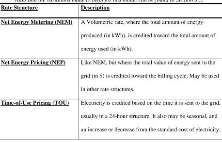
Table 2.1.1: These were the most common rate structures used in the relevant
literature, apart from a demand rate/charge. A more in-depth explanation into the rates and the variations made to them for this model can be found in Section 3.5. Rate Structure Description
Net Energy Metering (NEM) A Volumetric rate, where the total amount of energy produced (in kWh), is credited toward the total amount of energy used (in kWh).
Net Energy Pricing (NEP) Like NEM, but where the total value of energy sent to the grid (in $) is credited toward the billing cycle. May be used in other rate structures.
12
Real-Time Pricing (RTP) Based on the Real-Time Price of electricity, usually hourly rates. Can be affected by real-time events.
Day-Ahead Pricing (DAP) Forecasted electricity costs from utilities, like real-time price. Usually forecast the day before.
Additionally, much research on BES and rate structures focused on countries outside the US, largely seeking relief from higher electricity prices or emissions (Khalilpour, Vassallo, & Chapman, 2017). While providing useful information on the models used or background
information, these countries have different rate structures, electric grid structures, solar capacity, economics, etc.. Therefore, for results applicable to the economic situation, solar generation capabilities, and policy/rate structures, research from the US was prioritized.
2.2 Prior Research Results
The two resulting effects of battery energy storage that are discussed most in the current literature are the electricity cost reductions and emission reductions. Most cost reduction
analyses focus on specific consumers or rates to determine the cost effectiveness of operating or purchasing BES. Generally, the larger consumers that operate under demand rates have the greatest cost savings for BES. For reducing emissions, the consensus among researchers seems to be that unless designed specifically to lower emissions, BES will lead to increases in
13
Fisher & Apt (2017) and Griffiths (2019), modeled commercial and industrial customers that used BES across the country, to find the impacts on costs, emissions, and energy loads. The commercial and industrial customers did not have electricity generation on site for their energy profile, rather the model used for Griffiths (2019) used the battery solely for the building demand, while Fisher & Apt (2017) used energy arbitrage and demand reduction as the battery functions. Both models used a battery scaled to the power needs of the customers, which resulted in a much larger capacity than a residential sized battery. They found that in specific regions BES can mitigate emissions if a well-designed rate structure is implemented. Both recognize the rate structure needed involves a time-component based on the emissions of the region. They also recognize that a rate structure designed to reduce emissions is not necessarily the type of rate structure that provides the most revenue.
Results often indicated that positive effects like emission reduction were likely
14
2.3 Models of Battery Operation
Perhaps the most frequent problem with the research on battery energy storage, and microgrids in general, is that the battery operates in a very specific way for nearly all models. The battery either will not feed energy into the grid and only cover the local demand (such as in Griffith (2019)), or does not charge from local renewable energy, only from the grid (such as in Fisher & Apt (2017)). This poses a problem, as the goals of the Energy Storage Roadmap, time-shifting the residential renewable energy and managing the PV system, may require feeding energy from the residential solar system into the grid at a later time.
15
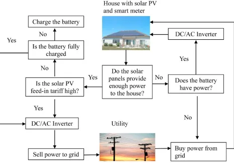
Figure 2.3.1: (Ren, Grozev, & Higgins, 2016). While the flowchart shows the
battery charging from solar (and references charging from the grid in the text), it does not discharge the battery to sell energy to the grid, only discharges to cover household demand.
16
Figure 2.3.2: (Nojavan, Majidi, Najafi-Ghaleloum Ghahramani, & Zare, 2017).
As seen in the grey circle, the battery storage only takes from the grid (or fuel cell/PV), and does not discharge back to the grid, only discharges to cover household demand.
Babacan et al. (2018) has a similar situation in Figure 2.3.3, specifically the scenario b, where the solar PV, Battery Energy Storage, and macrogrid are used to meet the household demand, and the battery is generally used for self-consumption of the generated PV Energy. However, Babacan (2018) also shows that in Figure 2.3.3 scenario c, the battery buying and
17
Fig. 2.3.3: (Babacan et al., 2018). Of the three models discussed in this research,
the only one that uses solar PV (PV Self-Consumption) does not sell energy to the grid, however the model that does sell energy to the grid (Energy Arbitrage) uses standalone storage.
18
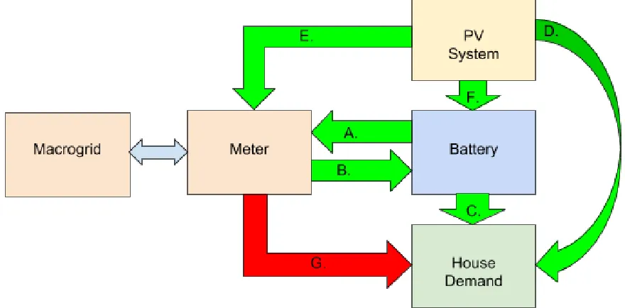
Figure 2.3.4: Model of the System Used. Upon investigation into the models of
the systems used in much of the research, one of two areas were found missing compared to the model used here. For the most part, smaller sized (residential) PV + Storage systems did not allow the battery to feed into the grid, or larger sized (standalone storage, usually for commercial, industrial, or distribution) did not have PV systems, but operated based on their demand charges from the grid and battery.This figure represents the 4 hubs of electricity usage/production within a home, and the 6 actions available to the homeowner, which are further explained in Table 3.2. The key aspect which is better illustrated in this figure is how the flow of energy between certain hubs is limited in one direction,
19
2.4 Research Question
20
3.
Methods
The goal of this system is to provide the most profit to the Solar + Storage prosumer. The subject in this method has a PV Solar Array and a Battery Energy Storage System and wants to operate it in the ways that are most profitable. Trying various rate structures will yield different ways to operate their BES, and the results can be compared with other rate structures. These results include the factors related to the goals laid out in the Energy Storage Roadmap. The model represents a single residential solar system with battery energy storage and runs a linear optimization to determine the battery charge/discharge operation, and energy taken from/sent to the grid. Using a variety of rate structures, it can determine how the residential solar customer would operate a BESS within their home to maximize their own profit with the different rate structures. The output from that optimization was then used to see how well the customer’s behavior matched the goals of the Energy Storage Roadmap based on the metrics mentioned in Table 3.3.1.
The process starts with optimizing for customer profit (Babacan et al., 2018) (Maleki, Rosen, & Pourfayaz, 2017). The monetary value to credit demand and production was based on different rate structures, run for each month, then summed over a year to simulate a customer’s annual electricity bill. Linear optimization was used to determine what actions the prosumer would make in order to maximize their profit with the battery. The outcomes or actions resulting from the optimization were then used to determine how well the new rate structures matched the goals of the Energy Storage Roadmap. This was determined by analyzing the use patterns and metrics based on ESR goals; the difference in CO2 emissions compared to a home with solar,
21
3.1 What actions the homeowner can take
There are essentially four different bodies within the model; the macrogrid/meter, the PV system, the battery, and the household demand. The homeowner has two inflexible conditions, the amount of energy that is produced by their solar array aka the PV System, and the energy needed for their home, aka the Household Demand. For these two bodies however, the energy may be sent/received to/from various places. The PV System may send energy to cover the Household Demand, to charge the battery, or send excess energy to the grid. The Household Demand may be covered by the PV System, the Battery, or from the grid. The homeowner has control over the battery operation, and any demand not covered by the battery or PV system must be taken from the grid.
It is important to note that the grid should not be receiving and delivering energy within the same hour. For example, when the PV system is producing energy the household demand must be met first, as the grid could not send energy and receive it. A single wire cannot allow flow in opposite directions at the same point in time. This is also true for the battery’s
charging/discharging. To use Figure 2.3.4 to explain, arrows A/C cannot be used at the same time as arrows B/F. Nor can arrows A/E be used at the same time as arrows B/G. While performing linear optimization, this type of constraint is difficult to process, as it is seemingly non-linear. To account for this difficulty, the model uses the ‘Big M’ method, explained with equations 5-15.
3.2 The Model
The model created for the battery operation requires well defined variables and
22
macrogrid, a way to balance the energy flowing in/out of the system, and the linear optimization equation to get the prosumer the maximum profit.
Variables
Pv = Solar Energy
Hd = Household Demand
Bc = Battery Charging Energy
Bd = Battery Discharging Energy
Bt = Battery Total Charge
Bcbin= Battery Charging Energy Binary
Constraint
Bdbin= Battery Discharging Energy Binary
Constraint
Fi = Financial Charge for Grid Energy into House (Demand Cost)
Fo = Financial Credit for Energy Sent out to Grid (Injection Credit)
Gi = Grid Energy into House
Go = Energy Sent to Grid
Gibin = Grid Energy into House Binary
Constraint
Gobin = Energy Sent out to Grid Binary
Constraint
M = For Use in the ‘Big M’ method
Me = Marginal Emission Factor
Ei = Efficiency Lost Increase
Ed = Efficiency Lost Decrease
RTP = Real-Time Price of Energy
h=hour
hi=initial hour
hf=final hour
Battery Physical Constraints
The constraints for the battery were taken from the Tesla Powerwall functionality (Tesla, 2019). A Tesla Powerwall was chosen for a variety of reasons; the popularity of Tesla, the comparable cost, and the use of Lithium-Ion rather than Lead-Acid. Batteries of similar capability are also used in much of the current research (Fridgen, Kahlen, Ketter, Rieger, & Thimmel, 2018) (Babacan et al., 2018). The Battery has a maximum charge/discharge (Bc/i) rate of 5 kW (Equations 1-2), and a maximum Capacity of 13.5 kWh (Equation 3).
0 ≤ 𝐵𝑐 ≤ 5 [1]
0 ≤ 𝐵𝑑 ≤ 5 [2]
0 ≤ 𝐵𝑡 ≤ 13.5 [3]
23
𝐵𝑡ℎ = 𝐵𝑡ℎ−1+ 𝐵𝑐ℎ∗ 𝐸𝑑 − 𝐵𝑑ℎ∗ 𝐸𝑖 [4]
Big M Method
The model uses the ‘Big M’ method for constraining the battery charging/discharging and grid energy flowing in/out of the house. The ‘Big M’ method is used in linear programming to create constraints on variables within the optimization that wouldn’t normally be viable for linear programming. Specifically, in this case some variables need to be 0 if a paired variable is greater than 0. To use the ‘Big M’ method, a new set of binary variables are created and paired with the original variables (Equations 6-9). These binary variables are summed, and the sum must be less than or equal to 1 (Equations 10-11). These paired binary variables are then multiplied with a number larger than they could theoretically be (Equation 5), to become the upper limit for the paired non-binary variables (Equations 12-15). This way, whichever variable is required to be 0 cannot exceed the zero value of the binary variable.
For this model, the ‘Big M’ method involves the Battery Charge (Bc)/Battery Discharge (Bd), and the Grid Energy Into House (Gi)/Energy Sent out to Grid (Go) for the two sets of paired binary variables (Xbin). This is to ensure the Battery cannot charge and discharge at the
same time and the Grid cannot both send and receive energy
𝑀 = 100 [5]
𝐵𝑐𝑏𝑖𝑛 = 𝑏𝑖𝑛 [6]
𝐵𝑑𝑏𝑖𝑛= 𝑏𝑖𝑛 [7]
𝐺𝑖𝑏𝑖𝑛 = 𝑏𝑖𝑛 [8]
𝐺𝑜𝑏𝑖𝑛 = 𝑏𝑖𝑛 [9]
0 ≤ 𝐵𝑐𝑏𝑖𝑛 + 𝐵𝑑𝑏𝑖𝑛 ≤ 1 [10]
0 ≤ 𝐺𝑖𝑏𝑖𝑛 + 𝐺𝑜𝑏𝑖𝑛 ≤ 1 [11]
0 ≤ 𝐵𝑐 ≤ 𝐵𝑐𝑏𝑖𝑛∗ 𝑀 [12]
0 ≤ 𝐵𝑑 ≤ 𝐵𝑑𝑏𝑖𝑛∗ 𝑀 [13]
0 ≤ 𝐺𝑖 ≤ 𝐺𝑖𝑏𝑖𝑛∗ 𝑀 [14]
0 ≤ 𝐺𝑜 ≤ 𝐺𝑜𝑏𝑖𝑛∗ 𝑀 [15]
Balanced Energy Equation
24
(Equation 16), where any energy flow needed for the system (Household Demand, Battery Charging, Energy into Grid) is taken from the energy flow into the system (PV solar, Battery Discharge, Grid into House).
(𝑃𝑣 + 𝐵𝑑 ∗ 𝐸𝑑 + 𝐺𝑖) − (𝐻𝑑 + 𝐵𝑐 ∗ 𝐸𝑖 + 𝐺𝑜) = 0 [16]
Unlike the Battery Total (Equation 4), the Battery Discharge (Bd) Efficiency is decreased (Ed), and the Battery Charge (Bc) Efficiency is increased (Ei). This is done to ensure the efficiency losses are correctly compensated for by the grid/solar/demand.
Optimization Equation
After all the constraints, the optimization equation is relatively simple. Maximize the sum of the consumer’s bill from the initial to the final hour (Equation 17). To get the consumer’s bill, multiply the Grid Into House Energy by the demand credit and subtracted from the Energy Sent To Grid multiplied by the injection credit.
max ∑ (𝐹𝑜ℎ𝑓ℎ𝑖 ℎ∗ 𝐺𝑜ℎ− 𝐹𝑖ℎ∗ 𝐺𝑖ℎ) [17]
3.3. Metrics:
After performing the linear optimization with Equation 17, the model now needs to determine the effects of the battery operation. This is done with various metrics, values based on the goals set forth in the Energy Storage Roadmap. These goals, seen in Table 3.3.1 below, are calculated from the data gathered after the optimization.
Table 3.3.1: A basic description of the goals of storage from the Energy Storage
Roadmap. ‘What the battery would do’ is a general description of the way the battery would need to function to match ESR Goals. Energy from discharging the battery could be used to cover the household demand or also to be sent into the grid.
ESR Goals What it means What the Battery would do
Cost Reduction Reduce Electricity delivery costs to the consumer and/or the utility
25 Emission
Reduction
Decrease the net CO2 Emissions
created by energy use from the home/battery
Charge while CO2 emissions are
low, discharge while emissions are high
Operate Microgrids
Increase grid resiliency, operate with little grid energy
Have increased battery Capacity, or decreased grid energy in.
Solar + Storage Management
Use BES to manage PV output Charge from the home solar system Limiting
Exported Energy
Reduce high demand and increase low demand
Charge when demand is low and discharge when demand is high Peak Demand Reduce peak demand from the
grid
Discharge the battery at high peak demands
Time-Shift Renewable Energy
Charge from renewables while they are producing and discharge when they are not
Charge from PV systems or Grid renewables, and discharge when not producing
Cost Reduction
The cost to the prosumer (Equation 18) is important to consider for any rate structure design. The Consumer Cost metric is the cost of buying/selling electricity to the utility and is dependent on each rate structure. The cost is determined by taking the grid energy in/out result of the monthly optimizations for each hour, multiplying each by their respective financial credits, and summing the hourly totals for the year. Thus, the consumer cost is the cost of buying/selling electricity from/to the grid for the year ($/yr.). The battery is used to minimize that cost
(maximize the profit). Thanks to the linear optimization, all that requires is the same
optimization equation, but negative to account for the metric being a cost rather than a bill credit as it was defined as in the model.
-∑ (𝐹𝑜ℎ𝑓ℎ𝑖 ℎ∗ 𝐺𝑜ℎ− 𝐹𝑖ℎ∗ 𝐺𝑖ℎ) [18]
26
difference between the Real-Time Price of energy and the Financial charges the prosumer pays or gets credit for.
∑ {(𝐺𝑖ℎ𝑓ℎ𝑖 ℎ∗ (𝑅𝑇𝑃ℎ− 𝐹𝑖ℎ) + 𝐺𝑜ℎ∗ (𝐹𝑜ℎ− 𝑅𝑇𝑃ℎ)} [19]
As seen in Equation 19, the prosumer pays the utility for Grid Energy into the Home (Gi), so the difference in price between the Real-Time Price (RTP) and the Financial Charge (Fi) is profit, whereas the prosumer gets credit for Energy Sent to the Grid (Go), so the difference between the Financial Credit (Fo) and the Real-Time Price (RTP) costs the utility. This equation provides the cost per hour for providing/buying energy to/from the home, and the metric is summed for the year ($/yr.).
The consumer and utility costs used only considers the cost of buying/selling the energy delivered to/from the home, i.e. the ‘delivery charge’ for electricity. It does not take minimum or fixed costs that would be present on a typical consumer bill into account. One such cost, a demand change, in not used in the model optimization. Demand charges are based on the highest electricity demand for the consumer, and apply a charge based on the amount used for that peak demand. This is a non-linear cost that was not included in the linear optimization model. Other fixed costs, minimum costs, or subsidies/credits would be independent of the optimization and applied to a consumer bill per month. These types of additional costs could be used to equalize differences in costs between rate structures that may otherwise have preferable operation patterns. Such changes in fixed costs should be considered by policy makers that wish to implement rate structures while mitigating costs to different entities.
CO2 Emission Changes
CO2 emissions for the modeled system are based on the Marginal Emission Factors for
27
(November - March), Summer (May - September), and ‘Transient’ (April & October). These hourly emission factors (Me) are multiplied by the hourly difference between Grid Energy into the Home (Gi); which is ‘dirty’ energy taken from the grid, and Energy Sent to Grid (Go); which is ‘clean’ energy from the battery or solar, thus reducing overall emissions. Summing this
annually gives a net value of marginal CO2 emissions (kg/yr.). Subtracting the annual marginal
emissions of a similar home with only a solar system shows the change in CO2 emissions
generated from the battery operation, where a positive value is an increase in emissions over a solar-only home, and a negative value is a decrease in emissions from a solar-only home.
∑ (𝑀𝑒ℎ𝑓ℎ𝑖 ℎ∗ {𝐺𝑖ℎ− 𝐺𝑜ℎ})− 𝑆𝑜𝑙𝑎𝑟𝐶𝑂2 [20]
While the energy sent to the grid from the battery may not have been ‘clean’ originally, if it was charged from the grid, that is compensated by the increase in emissions from when it did charge. Theoretically, the battery could be charged during periods of low emissions and discharged during high emissions in order to reduce overall emissions. This is explored later with the
‘Marginal Emission’ rate structure and the ‘Real-Time Price/Day-Ahead Price + Cost of Carbon’ rate structure.
Operate Microgrids (Increased Resiliency), Manage PV System, Limiting Exported Energy, Time
Shift Renewable Energy (Grid Average Daily Use Patterns)
Operating Microgrids/Increasing Resiliency can be measured by taking the average battery capacity (Equation 21) and the total energy taken from the grid (Equation 22). The average amount of energy stored in the battery is a good indicator of how readily the household can ‘island’ itself from the grid in the event of an outage.
28
However, the battery average capacity is not the only factor when determining microgrid
operation or increases in resiliency. When determining how effective the BES is at managing the PV output and how it limits exported energy, the model compares the amount of energy taken from/ sent into the grid across different rate structures (Equation 22). As the prosumer charges the battery from the solar and discharges to meet the demand, the amount of energy taken
from/sent to the grid decreases (kWh/yr.). However, if the prosumer charges from the grid (when prices are low) or sends the energy to the grid (when prices are high), the Grid In/Out totals will increase.
∑ℎ𝑓ℎ𝑖 𝐺𝑖ℎ, ∑ℎ𝑓ℎ𝑖 𝐺𝑜ℎ [22]
The average daily use patterns for the battery and grid also provide a clearer
understanding of how the battery operates in conjunction with the grid. These patterns are found by taking the average battery use (Equation 23) or grid use (Equation 24) for a 24 hour day.
𝐴𝑣𝑒𝑟𝑎𝑔𝑒𝑖𝑓(ℎ𝑖 − ℎ𝑓, ℎ𝑥, 𝐵𝑐ℎ− 𝐵𝑑ℎ) [23]
𝐴𝑣𝑒𝑟𝑎𝑔𝑒𝑖𝑓(ℎ𝑖 − ℎ𝑓, ℎ𝑥, 𝐺𝑖ℎ− 𝐺𝑜ℎ) [24]
The average daily use patterns are important when considering other metrics. For example, the average battery state of charge may be low for some rate structures because it uses the energy stored to meet the household demand through the day. This could lead to lower average battery state of charge, but still relatively high resiliency since it operates mostly independently of the grid. This would also be reflected in the total Grid In Energy (Equation 22]
Peak Demand/Injection
29
grid (or sent out to the grid if the rate incentivizes discharging during to the grid) at the highest points, provides valuable information on changes to the prosumer’s peak demand/injection. A lower peak demand/injection is more desirable, as it indicates more stable consumption. The time at which the demand/injection peaks is not a metric itself but provides insight to the underlying motivation/optimization that results in such battery behavior. Such information can also be seen by comparing the average daily use patterns. The peak demand/injection was found with Equation 25.
𝑃𝑒𝑎𝑘 𝐷𝑒𝑚𝑎𝑛𝑑 = max(𝐺𝑖), 𝑃𝑒𝑎𝑘 𝐼𝑛𝑗𝑒𝑐𝑡𝑖𝑜𝑛 = max (𝐺𝑜) [25]
3.4 Data Sources
The model created was of a residential prosumer with an average demand profile and average solar production for the region of Rochester, NY. The demand and PV production profiles for the home were needed to create such a model, as well as the relative size for a base case home. In this case, the average residential solar system installation size in NY is about 7.5 kW according to NYERDA NY-Sun Data and Trends residential data (NY-Sun, 2019). Inputting the average size and location (7.5 kW and Rochester, NY) into the PVWatts Calculator from NREL, gets the PV AC System Output (W) data column, as well as the hourly time and date for the year (NREL, 2016). At this point it is best to convert the AC system output to kW, as using kilowatts rather than watts will be beneficial in keeping a standard unit between the production, household demand, battery operation, and cost of electricity.
The next set of data gathered was the household demand data. This was taken from OpenEI’s dataset of the “NREL Commercial and Residential Hourly Load Profiles for all TMY3 Locations in the United States” using a base case load for a home in Rochester, New York
30
[kW](Hourly) is needed. Combining the annual data of the solar PV production and household demand required too much memory for the model and solver used in the analysis (OpenSolver, 2019) so the year was segmented into months. To create the annual rate structure, two columns for pricing were needed, one for the electricity consumed by the household from the grid and one for the electricity produced by the household sent to the grid. These changed with different modeled rate structures.
The Real-Time Price of Electricity is needed to calculate the utility costs, as well as for the Real-Time Price rate structures. This was found with LCG Consulting (2019) and NYISO Industry Data, using the Genese region for 2016 to correspond with our PV production data. The real time price of electricity gives a good indicator of the cost to utilities in providing, selling, and buying the electricity going to and coming from the residence. To calculate the CO2
emission reduction that the battery provides, the Marginal Emission Factors for Upstate NY were used. They have averaged hourly (0-23) CO2 emissions in kg/kW for 3 different seasons, Winter
(November-March), Summer (May-September), and Transition Seasons (April & October). By making any energy the home provides to the grid have negative emission factors (PV &
discharging the battery), and energy taken from the grid have positive emission factors (meeting demand & charging the battery), the model will then sum the annual results and determine the total emissions avoided by the residential system (See Equation 20).
The PV data, Household Demand Data, Real Time Price, and CO2 Emissions give the
31
3.5 Rate Structures
There are a variety of rate structures chosen for use in the model with various purposes. For residential homeowners in NYS, the most common rate structure is Net Energy Metering (NEM). This is a volumetric rate, where the total amount of energy produced (in kWh), is
credited toward the total amount of energy used (in kWh). NEM thus does not encourage the use of a BES, as the total amount of solar injected would be credited, and the efficiency losses of the battery would always result in less energy being credited. NEM is used frequently to encourage residential solar adoption, as an average home may greatly reduce their electricity bills with an average sized solar system. However, NEM may not fully capture the effects that the operation of residential solar has. Residential homes with solar often stop producing energy as demand for their homes and the macrogrid is spiking (later in the evening), leading to a drastic increase in demand from the grid. Despite this increase in overall demand from the macrogrid, there would not be an increase in pricing for NEM rate structures. As more and more homes install solar and are put on NEM rate structures, this may exacerbate the problem.
New York State permits residential homeowners to use NEM for a 20-year period after a solar installation. This provision is in place until 2020, but any change afterwards has not yet been announced. One potential change is to simply reduce the value of NEM by reducing the injection credit. This changes the rate from a volumetric rate to a monetary rate. This was
32
A potential alternative to traditional NEM proposed by NYS is the Value of Distributed Energy Resources (VDER) rate structure. There are many different ‘stacked’ variables that VDER uses to more accurately value the distributed generation of electricity. VDER has a Time-of-Use rate structure mentioned specifically in the Value Stack Calculator (VSC) to be used with BESS called the Capacity Alternative 2. This TOU rate would increase the value of energy between the hours of 2 PM – 7 PM during the months of June, July, and August. For use in the model, this rate was designed based on Net Energy Pricing (NEP), where the injection credit and demand costs are equal at any given point in time. Between the hours of 2 PM – 7 PM, this Capacity Alternative rate structure gave a 25% increase for both the injection credit and demand cost (Equations 26-28). This was done both for the originally defined summer months as well as annually.
VDER Capacity Alternative 2
0 ≤ ℎ𝑥 ≤ 13, 𝐹𝑜 = 𝐹𝑖 = $0.11 [26]
14 ≤ ℎ𝑥 ≤ 19, 𝐹𝑜 = 𝐹𝑖 = $0.13 [27]
19 < ℎ𝑥 ≤ 23, 𝐹𝑜 = 𝐹𝑖 = $0.11 [28]
VDER was originally designed for use during the summer season, but an annual
alternative could be created based on the marginal emission factors for the region, as well as the limits the battery would have. The rate structure created was called Marginal Emissions (ME), and used the 25% increase like VDER, but over different and shorter time periods for each season. These were 10 PM – 2 AM during the winter season (Equations 29-31), 12 PM – 4 PM during the summer season (Equations 32-34), and 11 AM – 3 PM during the transient months (Equations 35-37). These seasonal TOU rates can also be used with NEM during the off months, like the VDER Capacity Alternative operation in the summer.
ME Winter
0 ≤ ℎ𝑥 ≤ 1, 𝐹𝑜 = 𝐹𝑖 = $0.13 [29]
33
22 ≤ ℎ𝑥 ≤ 23, 𝐹𝑜 = 𝐹𝑖 = $0.13 [31] ME Summer
0 ≤ ℎ𝑥 ≤ 11, 𝐹𝑜 = 𝐹𝑖 = $0.11 [32]
12 ≤ ℎ𝑥 ≤ 15, 𝐹𝑜 = 𝐹𝑖 = $0.13 [33]
16 < ℎ𝑥 ≤ 23, 𝐹𝑜 = 𝐹𝑖 = $0.11 [34] ME Transient
0 ≤ ℎ𝑥 ≤ 10, 𝐹𝑜 = 𝐹𝑖 = $0.11 [35]
11 ≤ ℎ𝑥 ≤ 14, 𝐹𝑜 = 𝐹𝑖 = $0.13 [36]
15 < ℎ𝑥 ≤ 23, 𝐹𝑜 = 𝐹𝑖 = $0.11 [37]
Another Time-of-Use rate designed for BESS is the Smart Export rate structure, currently in use in Hawaii. This rate does not credit any injection of energy into the grid between the hours of 9 AM - 3 PM and otherwise uses net pricing at the standard rate (Equations 38-40). This drastically increases consumer costs and reduces utility costs, and the battery chosen does not have the capacity to store all solar electricity produced during this time. However, based on the previous testing with the NEM percentage alternatives, the rate structure would have similar performance if the credit between 9 AM – 3 PM was simply reduced to 81% of the standard rate rather than no credit at all (Equations 41-43). This rate structure could also be changed by altering the hours or seasons that it would be in use, which was done with the Smart Export 81% 11-1, June-August rate structure (Equations 44-46).
Smart Export
0 ≤ ℎ𝑥 ≤ 8, 𝐹𝑜 = 𝐹𝑖 = $0.11 [38]
9 ≤ ℎ𝑥 ≤ 3, 𝐹𝑜 = 0, 𝐹𝑖 = $0.11 [39]
4 ≤ ℎ𝑥 ≤ 23, 𝐹𝑜 = 𝐹𝑖 = $0.11 [40] Smart Export 81%
0 ≤ ℎ𝑥 ≤ 8, 𝐹𝑜 = 𝐹𝑖 = $0.11 [41]
9 ≤ ℎ𝑥 ≤ 3, 𝐹𝑜 = $0.08, 𝐹𝑖 = $0.11 [42]
4 ≤ ℎ𝑥 ≤ 23, 𝐹𝑜 = 𝐹𝑖 = $0.11 [43] SE 81% 11-1 J-A
0 ≤ ℎ𝑥 ≤ 8, 𝐹𝑜 = 𝐹𝑖 = $0.11 [44]
11 ≤ ℎ𝑥 ≤ 1, 𝐹𝑜 = $0.08, 𝐹𝑖 = $0.11 [45]
34
Real-Time Pricing (RTP) is a rate structure created using the actual energy price from the NYISO data, which is the price that the utilities pay for the energy they deliver (Equation 47). Day-Ahead Pricing (DAP) operates in much the same way, but the price is forecasted ahead of time (Equation 48). This leads to real-time pricing having more instability due to events that are not forecasted. The original RTP/DAP rates used net pricing, where the injection credit and demand costs were equal. An alternative was also tested with the model, using RTP/DAP for the injection credit and a standard flat rate for the demand costs (Equations 49-50). RTP/DAP prices are generally lower than the consumer demand cost, and if the prices are higher it is because the grid demand is much higher than normal. The RTP/DAP rates did not reduce emissions well, so another rate structure was created using both the RTP/DAP prices while adding on a cost of carbon. Using the marginal emissions (kg/kW) multiplied by the cost of carbon ($/kg) and added to the RTP/DAP rates created the RTP/DAP + Cost of Carbon rate structures (Equations 51-52).
Real-Time Price
𝐹𝑜 = 𝐹𝑖 = 𝑅𝑇𝑃 [47] Day-Ahead Price
𝐹𝑜 = 𝐹𝑖 = 𝐷𝐴𝑃 [48] RTP Flat Demand
𝐹𝑜 = 𝑅𝑇𝑃, 𝐹𝑖 = $0.11 [49] DAP Flat Demand
𝐹𝑜 = 𝐷𝐴𝑃, 𝐹𝑖 = $0.11 [50] RTP + Cost of Carbon
𝐹𝑜 = 𝐹𝑖 = 𝑅𝑇𝑃 + 𝐶𝑜𝑠𝑡 𝑜𝑓 𝐶𝑎𝑟𝑏𝑜𝑛 ∗ 𝑀𝑎𝑟𝑔𝑖𝑛𝑎𝑙 𝐸𝑚𝑖𝑠𝑠𝑖𝑜𝑛𝑠 [51]
DAP + Cost of Carbon
𝐹𝑜 = 𝐹𝑖 = 𝐷𝐴𝑃 + 𝐶𝑜𝑠𝑡 𝑜𝑓 𝐶𝑎𝑟𝑏𝑜𝑛 ∗ 𝑀𝑎𝑟𝑔𝑖𝑛𝑎𝑙 𝐸𝑚𝑖𝑠𝑠𝑖𝑜𝑛𝑠 [52]
35
36
4.
Results
4.1 Time-Shift & Annual Daily Averages
38
Figure 4.1: Shown here are the annual (except for Marginal Emissions, which
varied by season) Average Daily Use Patterns for the rate structures analyzed, along with some of their adjusted/changed rates that provided interesting/useful results. For each graph, the green solid line represents the battery operation, positive being charged, negative being discharged, and the red dashed line
represents energy from the grid, positive energy fed into the house, negative being sent out to the grid. The x-axis is the time of day (0-23), and the y axis is the kW being used by the battery/grid.
Discussion of Rates based on Average Daily Use (Figure 4.1)
For Net Energy Metering (NEM, Figure 4.1.1), the model found that if NEM credits the production of energy above 81% of what it charged, then the model did not operate the battery. Thus, as energy is produced by the solar it is sent to the grid.However, if the value of the credit for production fell to or below 81%, the desired behavior shifted, as we see in 81% Net Metering (Figure 4.1.2). The same concept was also applied to the VDER rate structure, to find at which point above 100% the changes in behavior take place, and it was found that an increase of 23% or more would change the optimization result. Thus, any rate structure proposed will need to take the efficiency of the battery, given that a 90 % efficiency means rate changes between 82-122% will not change behavior. As battery technology improves, this range should decrease. At the 81% injection credit for NEM, the battery is used to charge during solar production as much as possible, with excess production being sent to the grid. The battery is then discharged later to cover some of the household demand. This is a great example of microgrid operation and managing the PV system output, which can also be seen later in Table 4.2.1.
39
drain and take energy from the grid immediately after 7 PM. These sharp peaks are not desired behavior, as discussed with the peak effects.
The next set of rate structures in Figure 4.1 are the Real-Time Price (RTP) rates, which are more unstable than NEM. The first RTP (Figure 4.1.4) rate used a Net Energy Pricing (NEP) structure, where both the credit for production and cost for energy were the same. This led to a scenario where the battery didn’t charge from the solar as much, but rather from the grid when the energy was less expensive during the morning. The RTP Flat Demand rate changes the rate to only credit injected energy at the Real-Time Price and instead charge the normal price of energy for energy from the grid (Figure 4.1.5). RTP Flat Demand functions almost the same as 81% NEM, charging during solar production then discharging later to cover some of the
household demand, with a small difference around 11 AM. Given the battery charges less at this point on average, it can be assumed that the price of energy at 11 AM may be high enough occasionally to be worth inserting energy into the grid. Finally, the last of the Real-Time Price rates is the RTP + Cost of Carbon (Figure 4.1.6). This rate structure is created by combining the Real-Time Price of Energy with the Cost of Carbon (Zeng et al., 2018). This rate structure seems to follow the same general pattern as the normal RTP but is slightly more unstable. This
increased instability may be due to the seasonal changes in the marginal emission factors
affecting the cost of carbon. Because these are annual averages, the seasonal changes may affect the annual average stability.
40
However, when comparing RTP to DAP, we notice some irregularities. One example is at 8 PM the RTP rate encourages battery discharge, indicating higher prices, while the DAP does not. While this could be chalked up to the instability inherent in RTP, these patterns are averaged over a year, which means it is more likely that the DAP forecast is missing a peak demand at 8 PM, causing spikes in the RTP. A similar trend occurs at 5 AM.Like the normal DAP and RTP, the overall pattern for the flat demand rates (Figure 4.1.8) are similar, but again with slight differences. The slight peak at 11 AM from the RTP still there, but the battery has a smoother transition over that point.The differences between the DAP/RTP + Cost of Carbon (Figure 4.1.9) are hard to discern due to the more chaotic patterns but seem to be comparable to the differences between the regular RTP/DAP, with shifts at 5 AM and 8 PM.
The rate structure is Smart Export (Figure 4.1.10), used in Hawaii and developed for battery energy storage. The structure credits the production of energy at $0 from 9 AM – 4 PM, and equal to the demand between 4 PM – 9 AM, while demand remains consistent through the day. For this rate, the model shows an increase in battery charging from the solar during the day, and overall decreases in energy taken from the grid. Like the NEM analysis (4.1.1), the Smart Export 81% (Figure 4.1.11) shows that changing the production value from 0% of the demand to 81% does not change the pattern of behavior. Changing the time period (Figure 4.1.12) from 9 AM- 4 PM to 11 AM – 2 PM has a very significant effect. While the beginning and end of the day have similar grid use, if slightly increased due to less BES charging, the sharp peaks between sending energy to the grid and charging the battery are very pronounced.
41
the marginal emission factors. In the winter (Figure 4.4.13), this is between 10 PM- 2 AM, the summer (Figure 4.1.14) 12 PM – 4 PM, and the transient season (Figure 4.1.15) 11 AM – 3 PM. With each season there are different battery and grid trends to accommodate this. In the winter, there is increased demand at night, as the battery charges during the day to discharge later. In summer, the battery charges in the morning, and later has very high discharge rates during the afternoon. The transient season is very similar to the summer due to the similar time frames.
4.2 Rate Variations
The six main rate structures, Net Energy Metering (NEM), Value of Distributed Energy Resources (VDER), Marginal Emissions (ME), Smart Export (SE), Real-Time Price (RTP), and Day-Ahead Price (DAP), all had various variations used to either compare to another rate or achieve a better metric of an ESR goal. The tables and charts in this section explain the
reasonings behind the variations to the base rate structures, and how they ended up comparing to the original.
Net Energy Metering
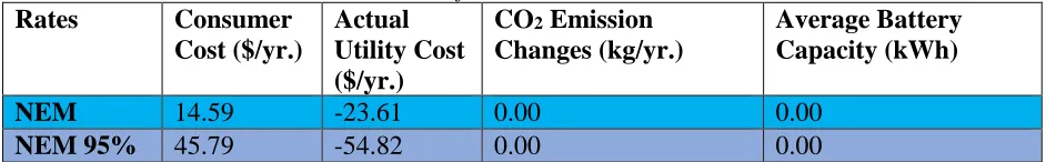
Table 4.2.1: Metrics for Net Energy Metering (NEM) rate structures. Rates
highlighted in blue have injection credit above 81%, rates highlighted in orange have injection credit 81% or below. The blue rates do not operate the BES, while the orange rates all operate in the same manner. The Net Energy Metering rate, due to the battery efficiency losses, would not cause the battery to be used unless injection credit fell below 81% of the demand charge, and the battery starts at 0 kWh for the model. Therefore, NEM rates above 81%, the battery capacity is 0 kWh. Once the price was low enough, the battery operated by charging from the solar and discharging later to cover the household demand (See also: Figure 4.1.2). Once the NEM credit was below 81%, the battery was operating in the most profitable way, as the credit did not change over time, hence the consistent values between rates aside from the Consumer/Utility Cost. This differs from the other rates, which are based on a Time-of-Use rate structure.
Rates Consumer Cost ($/yr.)
Actual Utility Cost ($/yr.)
CO2 Emission
Changes (kg/yr.)
Average Battery Capacity (kWh) NEM 14.59 -23.61 0.00 0.00
[image:42.612.71.542.637.710.2]42
NEM 90% 77.00 -86.02 0.00 0.00
NEM 85% 108.20 -117.23 0.00 0.00
NEM 81% 131.45 -117.22 330.88 5.77
NEM 75% 144.92 -130.68 330.88 5.77
NEM 50% 201.01 -186.77 330.88 5.77
NEM 25% 257.09 -242.86 330.88 5.77
Grid In (kWh/yr.) Grid Out (kWh/yr.) Peak Grid In (kW) Peak Grid In Time Peak Grid Out (kW) Peak Grid Out Time NEM 5969.05 5832.72 2.41 7:00 PM 5.20 12:00 PM
NEM 95% 5969.05 5832.72 2.41 7:00 PM 5.20 12:00 PM
NEM 90% 5969.05 5832.72 2.41 7:00 PM 5.20 12:00 PM
NEM 85% 5969.05 5832.72 2.41 7:00 PM 5.20 12:00 PM
NEM 81% 2926.96 2096.81 2.41 7:00 PM 5.14 12:00 PM
NEM 75% 2926.96 2096.81 2.41 7:00 PM 5.14 12:00 PM
NEM 50% 2926.96 2096.81 2.41 7:00 PM 5.14 12:00 PM
NEM 25% 2926.96 2096.81 2.41 7:00 PM 5.14 12:00 PM
Based on the Consumer and Utility Cost of the NEM rate structures, the battery operation can provide a significant consumer savings if the injection value decreases. Between 82-100%, every 1% decrease in injection value causes about a $6 increase in consumer cost, but when the battery operates below 81% injection credit, each 1% decrease only increases consumer cost by $2. These increases in Consumer Cost are the same decrease in Utility Costs, but once the injection credit is low enough that battery begins to operate, the Utility’s Costs increase slightly. The battery usage does not significantly change within the 81% group, as between 25%-81% the credit is low enough that the battery efficiency losses don’t matter, meaning the battery is already operating at maximum profit by increasing the homeowner’s self-consumption of electricity. Between 81%-100% credit, the battery is not used as the efficiency losses incurred would lower the profit compared to simply feeding in any excess solar.
43
(from the solar) as it requires from the grid, the emissions are very low. This makes sense, as the marginal emission factors can be higher during the day when the solar is producing and lower at night when the house draws energy from the grid, thus reducing the systems net emissions. However, when the battery operates, the Grid In energy is decreased by 3,736 kWh/yr., while the Grid Out energy is decreased by only 3,042 kWh/yr., meaning a difference of 694 kWh/yr. energy is lost due to the battery efficiency. This energy lost leads to an increase in emissions roughly equal to the difference between the CO2 Emissions for the two rates.
[image:44.612.68.545.556.703.2]Despite the increased cost and emissions, the NEM 81% was a great example of the ESR goals of microgrid operation, PV management, and limiting exported energy. The Grid In/Out energy is greatly reduced from standard NEM, from charging the battery from the solar and using that energy to meet the household demand. The Average Battery Capacity is above zero, making it better for microgrid operation. And while the Peak Grid In/Out for the NEM rates do not change significantly, with only a minor reduction in the Peak Grid Out, they do not increase as seen in later rates.
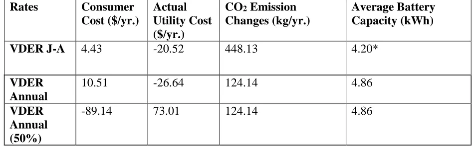
Table 4.2.2: Metrics for the Value of Distributed Energy Resources (VDER) rate
structures. The Value of Distributed Energy Resources rates were based on the VDER Alternate Capacity Option Two, where between 2 PM – 7 PM energy for both injection and demand have increased value, for 25% above the standard rate, and 50% for VDER Annual (50%). This rate was proposed to occur between June-August, using NEM the rest of the year, but was also extended throughout the year for the VDER Annual rate structure.
Rates Consumer Cost ($/yr.)
Actual Utility Cost ($/yr.)
CO2 Emission
Changes (kg/yr.)
Average Battery Capacity (kWh)
VDER J-A 4.43 -20.52 448.13 4.20*
VDER Annual
10.51 -26.64 124.14 4.86
VDER Annual (50%)
44 Grid In (kWh/yr.) Grid Out (kWh/yr.) Peak Grid In (kW) Peak Grid In Time Peak Grid Out (kW) Peak Grid Out Time VDER J-A
6106.25 5714.31 7.18 8:00 PM 8.74 2:00 PM
VDER
Annual 7176.69 6026.24 7.55 8:00 PM 9.08 2:00 PM
*VDER J-A Average Battery Capacity is measured during June-August, the rest of the year it is ‘zero’.
VDER June-August and VDER Annual had comparable Consumer and Utility Costs, where the $6.08 increase in Consumer Cost is the same decrease in Utility Cost. Testing was done on the increases of the percent change for the TOU rate (seen with VDER Annual (50%)), but a greater percentage had higher Utility Costs, making the rates less competitive with the standard NEM rate. The example shown above used a 50% rate instead of the 25%, which gave a $4 cost decrease to consumers and increase to utilities per 1% increase. Also, prices were only effective after a 23% increase due to battery efficiency, like the 81% decrease tested with NEM. The Peak Grid In/Out times shifted from NEM’s due to the time period of the rate structure; at 8 PM when costs went down, the battery charged from the grid, and at 2 PM when injection credit was high, the battery and solar both injected into the grid.
However, beyond the Consumer/Utility Costs and Peak Grid times, the differences for VDER June-August and VDER Annual are very significant. The Grid In/Out energy is increased for the annual rate, as is the Peak Grid In/Out energy. The CO2 emissions are greatly increased
45
Increased charging from the grid as opposed to the solar system means increased emissions, increased peak demand, increased exported energy, poor microgrid operation (requiring energy from the grid), and poor PV management. This can be seen comparing the VDER rate structure effects with the NEM’s. There is an increase in VDER’s grid in/out energy, increases for the Peak Grid In/Out energy, and increases in emissions. In this regard, VDER June-August seems to be the better rate of the two, with better metric results for meeting the goals of the ESR.
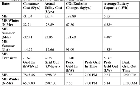
[image:46.612.72.542.399.690.2]Marginal Emissions
Table 4.2.3: Metrics for the Marginal Emissions (ME) rate structures. The
Marginal Emissions rate structures were created for use in the model and based on the VDER rate. As reducing emissions is a key goal of the Energy Storage Roadmap, and the VDER rates used were originally intended to be used only in summer, the annual VDER rate structure did not do a great job reducing
emissions. Therefore, using the same concept, a 25% increase over a set period of hours, a new TOU rate structure was created. This rate structure used the three seasons that were used for the marginal emission factors, Winter, Summer, and Transient. It was also used to create TOU rates for each season individually that used NEM for the rest of the year, again like VDER.
Rates Consumer Cost ($/yr.)
Actual Utility Cost ($/yr.)
CO2 Emission
Changes (kg/yr.)
Average Battery Capacity (kWh) ME -31.04 35.14 199.89 5.55
ME Winter
(N-Mr) 32.21 -28.59 67.80 6.58*
ME Summer
(M-S) -32.41 23.86 121.69 4.48*
ME Summer
(J-A) -14.72 -12.66 91.09 4.32*
ME
Transient -1.67 -7.35 10.40 5.66*
Grid In (kWh/yr.) Grid Out (kWh/yr.) Peak Grid In (kW) Peak Grid In Time Peak Grid Out (kW) Peak Grid Out Time ME 7845.46 6698.08 7.56 7:00 PM 9.63 12:00 PM
ME Winter
46
ME Summer
(M-S) 6732.28 6170.86 7.18 8:00 PM 9.47 12:00 PM
ME Summer
(J-A) 6394.88 6002.85 7.18 9:00 PM 9.44 1:00 PM
ME
Transient 6511.47 6205.66 7.11 8:00 PM 9.63 12:00 PM
*ME Winter, Summer (M-S & J-A), and Transient Average Battery Capacity is measured seasonally, the rest of the year they are ‘zero’.
The Marginal Emissions rate structures are difficult to compare to one another. Unlike NEM or VDER, there does not seem to be one rate structure superior to the others. Like VDER, the ME rates suffer from charging the battery from the grid, with higher Grid In/Out and Peak Grid In/Out energy than NEM, as well as increased CO2 emissions. Looking at Figure 4.2.4
below can help narrow down the better rates. The ME Summer June-August and ME Transient rates seem to be the ‘best’ of the ME rates used, as both have negative Consumer and Utility Costs, as well as lower emissions. However, the much greater emissions of the ME Transient rate structure seem to give it the edge between the two. Going back to table 4.2.3 shows that the Grid In/Out energy is slightly higher for the ME Transient, which may make the ME Summer June-August rate the more desirable. The close comparison between these two rates is a good example of one of the problems with the ESR; it doesn’t specify which goals have priority for residential prosumers with storage. However, for the purposes of future comparison, the ME transient is possibly the best of the Marginal Emissions rate structures, due largely to the lower CO2
47
Figure 4.2.4: Costs and Emissions Metrics for the Marginal Emissions (ME) rate
structures. Negative Costs and Emissions signify a better rate. Consumer/Utility Costs and CO2 Emission Changes are the displayed metrics.
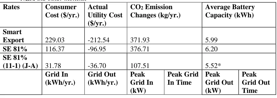
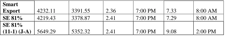
Smart Export
Table 4.2.5: Metrics for the Smart Export (SE) rate structures. The Smart Export
Rate Structure is used in Hawaii for consumers with Energy Storage, and values energy injected between 9 AM – 3 PM at $0. The SE 81% uses the principle from the NEM 81% and increases the injection value to 81% of the demand, which causes very little change to the consumer behavior, but gives a much fairer value to the consumer. The SE 81% (11-1) (J-A) shortens the length of time energy is credited to 11 AM – 1 PM and only applies the rate between June-August, using NEM the other months.
Rates Consumer Cost ($/yr.)
Actual Utility Cost ($/yr.)
CO2 Emission
Changes (kg/yr.)
Average Battery Capacity (kWh) Smart
Export 229.03 -212.54 371.93 5.99
SE 81% 116.37 -96.95 376.71 6.20
SE 81%
(11-1) (J-A) 31.78 -36.70 107.51 5.52*
[image:48.612.73.542.559.725.2]48
Smart
Export 4232.11 3391.55 2.36 7:00 PM 7.33 8:00 AM
SE 81% 4219.43 3378.87 2.41 7:00 PM 7.29 8:00 AM
SE 81%
(11-1) (J-A) 5649.29 5352.32 2.41 7:00 PM 9.08 2:00 PM
*SE 81% (11-1) (J-A) Average Battery Capacity is measured during June-August, the rest of the year it is ‘zero’.
The Smart Export 81% rate is better than the Smart Export rate, but mostly due to the decreased consumer cost. And this benefit is negated if utility costs are of higher priority. This shouldn’t be surprising, as the pattern of behavior for the two is nearly identical, but the Smart Export essentially gives the utility free energy from excess solar produced. Smart Export 11 AM – 1 PM June-August was used to see how shortening the time period and months applied would affect the rate, like the VDER and ME rates. There are a few key differences between the metrics of the Smart Export rates that provide interesting insight into the optimization. For example, the peak grid out time is 8 AM for the Smart Export and SE 81%. This happens because 8 AM is the hour before injection credit is reduced, which means having the battery discharge at this point. The slight difference in Average Battery Capacity occurs because the Smart Export discharges some excess energy during the day, as that energy is valued at zero anyway, making the Average Battery Capacity slightly lower. It is also lower in the SE 81% (11-1) (J-A) because of the shorter period it would charge in.
[image:49.612.72.543.71.147.2]Real-Time Price
Table 4.2.6: Metrics for the Time Price (RTP) rate structures. The
Real-Time Pricing uses the Actual Energy Price for the injection and demand charges, while the RTP flat demand uses the Actual Energy Price for injection credit only. The RTP + Cost of Carbon rate adds a social cost of carbon ($40/kg) using the marginal emission factors to the Actual Energy Price for the injection and demand charges.
Rates Consumer Cost ($/yr.)
Actual Utility Cost ($/yr.)
CO2 Emission
Changes (kg/yr.)
49
Real-Time
Pricing -212.18 0.00 751.39 6.47
RTP Flat
Demand 207.53 -277.31 350.39 5.69
RTP + Cost
of Carbon -197.84 -8.55 363.43 6.47
Grid In (kWh/yr.) Grid Out (kWh/yr.) Peak Grid In (kW) Peak Grid In Time Peak Grid Out (kW) Peak Grid Out Time Real-Time
Pricing 14077.35 11934.20 7.67 7:00 PM 9.83 12:00 PM
RTP Flat
Demand 3178.82 2291.89 2.41 7:00 PM 9.73 12:00 PM
RTP + Cost
of Carbon 12277.03 10614.00 7.00 6:00 PM 9.44 11:00 AM
The Real-Time Pricing rate structure had a huge decrease in the Consumer Cost, due to the many opportunities the battery had to make a profit buying and selling energy solely from the grid. This can be seen not only in Figure 4.1.4, but also the Grid In/Out energy in Table 4.2.5. As with the VDER and Marginal Emissions rates, charging the battery from the grid lead to poor metrics compared to NEM. The significant difference between Real-Time Pricing and NEM led to the rate RTP Flat Demand, which would operate like NEM 81% but discharge the battery into the grid when electricity is valued significantly high enough. However, this did not occur often enough to be profitable for the consumer (although like Smart Export, the consumer’s loss is the utilities gain). While attempting to bring down the huge increase in CO2 emissions from the
Real-Time Pricing rate, the rate was combined with a social cost of carbon based on the marginal emission factors. Interestingly, this drastically reduced CO2 emissions, while affecting the other
metrics only slightly.
[image:50.612.76.545.71.285.2]Day-Ahead Price
Table 4.2.7: Metrics for the Ahead Price (DAP) rate structures. The