Universal design framework for optimal application of chemical monolayer to open water surfaces

(1)

University of Southern Queensland

Faculty of Engineering & Surveying

Universal Design Framework for optimal application of

chemical monolayer to open water surfaces

A thesis submitted by

Gavin Neil Brink

in fulfilment of the requirements of

Doctor of Philosophy

(2)

Abstract

Annual evaporation losses from farm water storages in Australia typically exceed 40% of their storage volume. Potentially chemical films such as monolayers are an

economi-cal low-impact means of reducing evaporative loss, however, their performance has been shown to be highly variable. They are affected by a number of climatic and

environ-mental factors, principally wind-induced drift, deposition on the lee shore, submergence by waves, volatilisation and bio-degradation. Although these limitations must be

ac-commodated for in the management of the applied monolayer by means of appropriate and timely autonomous application, these limitation will vary for every location. Every

given site will have its own unique characteristic climatic and environmental factors. It is this variability that presents major difficulties to the general one-size-fits-all design

approach. Hence, to achieve optimal evaporation mitigation performance the develop-ment of a methodology to inform the design, installation and operation of a tailored

monolayer application system for any given site was seen as essential.

This thesis reports the conception, development and desktop evaluation of a Universal

Design Framework (UDF) to optimise the use of monolayer materials for evaporation mitigation. The UDF is designed to inform: (i) the most appropriate choice of

mono-layer material; (ii) the optimal type of application system and the site-specific config-uration required; (iii) the amount and re-application rate of monolayer to be applied;

and hence (iv) the expected performance of the application system. The UDF incor-porates all the necessary information with respect to water storage geometry, monthly

climate data (in particular, detailed wind statistics), water quality and biological fac-tors plus user performance criteria (the desired extent and duration of coverage). This

(3)

ii

1. Monolayer material is selected via a decision table, which allows the user to make comparisons between three previously benchmarked South East Queensland

(SEQ) reservoirs and their own, to determine a best match monolayer material.

2. Application system design is determined using a simulation platform, which al-lows the user to predict surface coverage and application rate according to wind

conditions via an iterative process in which the number and/or location of appli-cators may be varied until user performance criteria are met.

3. Likewise application strategies, namely which applicators to apply from and their

respective application rate for each wind condition, are also determined with the simulation platform for detailed wind conditions (both strength and direction) to

create a decision table. This table forms the basis for real-time (hour-by-hour) decision and control when the system is installed on-site, and

4. system performance is calculated for monthly site-specific wind statistical data

(using the simulation platform), and compared with user performance criteria to determine which months are suitable for application and monthly monolayer cost.

The simulation platform and the algorithms used to calculate firstly, the spreading rate and spreading pattern of monolayer (without wind stress), and secondly the drift rate,

spreading rate and spreading pattern of monolayer (with wind stress), are described. In order to calibrate the algorithms, and to research the requirements for (both current

and future) monolayer material characterisation, an empirical study for the commonly used evaporation-retarding monolayer stearyl alcohol (‘C18OH’ as a water-emulsion)

was undertaken. This involved the analysis of its observed spreading performance under different application and windspeed conditions on an indoor 6 m diameter tank with

controlled airflow.

Finally the scope of the UDF is discussed with regard to design, planning, installation and also daily, hour-by-hour management of monolayer application. This was informed

(4)

Publications

The following journal and conference papers, patent and research report have been

published or are in preparation for submission about the research contained within this dissertation.

Journal

Brink, G., Symes, T. and Hancock, N. (2011), ‘Development of a ‘smart’ monolayer

application system for reducing evaporation from farm dams introductory paper’, Australian Journal of Multidisciplinary Engineering. [In press]

Brink, G., Wandel, A., Hancock, N., Herzig, M. and Pather, S. (2011), ‘Spreading rate

and dispersion behaviour of evaporation-suppressant monolayer. Part 1 zero wind stress’, Water Resources Research. [Prepared: to be submitted with Part 2 following]

Brink, G., Wandel, A., Hancock, N. and Pather, S. (2011), ‘Spreading rate and dis-persion behaviour of evaporation-suppressant monolayer. Part 2 wind stress’, Water

Resources Research. [In preparation]

Brink, G., Hancock, N. and Pather, S. (2011), ‘Universal Design Framework for op-timal application of chemical monolayer to open water surfaces’, Agricultural Water

(5)

Publications iv

Conference

Brink, G., Wandel, A., Pittaway, P., Hancock, N. and Schmidt, E. (2011), Optimising

the design, installation and operation of a monolayer application system on a farm dam via a ‘Universal Design Framework’. Australian Irrigation Conference and Exhibition

2011, 22-25 August, Launceston, Australia. [Accepted for presentation]

Schmidt, E., Brink, G. and O’Shannassy , G. (2011), Application systems for

opti-mal management of monolayer. Urban Water Security Alliance Science Forum, 14-15 September, Brisbane, Australia. [Accepted for presentation]

Brink, G. (2011), Optimising monolayer application system design, installation and

operation on agricultural reservoirs through the use of a ‘Universal Design Framework’. Water Panel’s Post-Graduate Presentation Evening, 18 May, Brisbane, Australia.

Brink, G., Wandel, A., Pittaway, P., Hancock, N. and Pather, S. (2010), A ‘Uni-versal Design Framework’ for installation planning and operational management of

evaporation-suppressing films on agricultural reservoirs. International Conference on Agricultural Engineering, 6-8 September, Clermont-Ferrand, France.

Brink, G., Wandel, A., Pittaway, P., Hancock, N. and Pather, S. (2010), Determining

operational requirements to optimise monolayer performance on a farm dam via a ‘Universal Design Framework’. Australian Irrigation Conference and Exhibition 2010,

8-10 June, Sydney, Australia.

Symes, T. and Brink, G. (2010), A scalable distribution system for the optimal

appli-cation of evaporation suppressant film to farm dams. Australian Irrigation Conference and Exhibition 2010, 8-10 June, Sydney, Australia.

Brink, G., Wandel, A., Hancock, N. and Pather, S. (2009), Towards adaptive

oper-ational requirements for optimal application of evaporation-supressing monolayer to reservoirs via a ‘Universal Design Framework’. International Workshop on

(6)

Publications v

Brink, G., Symes, T. and Hancock, N. (2009), Development of a ‘smart’ monolayer

application system for reducing evaporation from farm dams introductory paper. CIGR International Symposium of the Australian Society for Engineering in Agriculture,

13-16 September, Brisbane, Australia.

Brink, G., Hancock, N. and Pather, S. (2009), ‘Smart’ monolayer application and management to reduce evaporation on farm dams - formulation of a universal design

framework. WaterTAPs Presentation, 1 June, Toowoomba, Australia.

Brink, G., Symes, T., Pittaway, P., Hancock, N., Pather, S. and Schmidt, E. (2009),

Smart monolayer application and management to reduce evaporation on farm dams - formulation of a universal design framework. Environmental Research Conference,

10-13 May, Noosa, Australia.

Patent

Brink, G. N. and Symes, T. W. (inventors) (2010), Evaporation inhibitor application.

[lodged April 2010]

Research Report

(7)

Certification of Dissertation

I certify that the ideas, designs and experimental work, results, analyses and conclusions

set out in this dissertation are entirely my own effort, except where otherwise indicated and acknowledged. I also certify that the work is original and has not been previously

submitted for assessment in any other course or institution, except where otherwise stated.

Gavin Neil Brink 0050083224

Signature of Candidate Date

ENDORSEMENT

(8)

Acknowledgments

Firstly I want to thank my family. Without their eduction, guidance, sacrifice, love

and support I would not have had the opportunities I have been so lucky to have. I can’t thank them enough. I would also like to thank my beautiful, strong and loving

girlfriend who has stuck with me throughout all of the highs and lows.

A big thank you to Erik Schmidt at the NCEA, who I first spoke with back in 2006

about monolayers, and since then has provided and created for me many opportunities over the years. Thanks you to my supervisors Associate Professor Nigel Hancock and

Dr Selvan Pather for their invaluable guidance, patience, belief and assistance. Also a big thanks to Dr Andrew Wandel from FoES for his help, guidance and assistance with

the development of the simulation and in finalising journal papers.

I appreciate the advice and support from FoES and NCEA staff, particularly Dr Pam Pittaway, my neighbour for a while there, has always helped to put things into

perspec-tive for me. Thank you for convincing me to stick with it. Also, thank you to Geoff O’Shannassay for all of his help with the monolayer work. Unfortunately, I can’t thank

Troy Symes in person today as he passed away last year, but I appreciate all he did for me.

Thank you to Michael Herzig for all of his effort in the development and formulation of a suitable monolayer material for testing and for his invaluable discussions on the finer

points of physical chemistry. On this point, I would also like to thank the ever so wise Emeritus Professor Geoffrey Barnes for his insightful discussions and his unwavering

(9)

ACKNOWLEDGMENTS viii

During my time at USQ I have made many friends both professionally and socially

from all over the world of whom I wish to thank for their support, specifically, Nicholas Stuckey, Dr Xavier Burgos, Dr Belen Gallego, Professor Victoriano Martinez, Nicholas

Roberts, Nishant Pradhan, Adrian Blockland, Mohan Trada and Terry Byrne.

Finally I acknowledge the Australian Postgraduate Award scholarship funding provided to me by the Australian Government. Also the Cooperative Research Centre for

Irri-gation Futures for their invaluable project funding, conference and travel support and post-graduate events.

Gavin Neil Brink

University of Southern Queensland

(10)

List of Figures

1.1 Block diagram of dissertation overview. . . 8

2.1 The relationship between the area occupied (˚A2) per molecule and the surface pressure (π) exerted by the film. (a) refers to the gaseous film

phase, (b) the liquid-expanded phase, and (c) the solid phase. Although the liquid-condensed phase is not shown here, this phase is similar to the

solid, however, the molecules are oriented diagonally instead of vertically. Reproduced from Gladyshev (2002). . . 14

2.2 Diagrammatic illustration of the physics of thermal transport processes:

(a) details the atmospheric and liquid layers; (b) details the gaseous boundary layer and liquid diffusion sublayer near the interface.

Repro-duced from Hancock, Pittaway & Symes (2011). . . 20

2.3 Degradation of three monolayer compounds supplied as the sole carbon

source for the common freshwater bacterium Acinetobacter in a mineral salts medium. The resilience of two fatty alcohols (C16OH, C18OH) and

a ethylene glycol monooctadecyl ether (C18E1) monolayer were com-pared. Chloroform was used to extract the monolayer in the medium

after two, three and four days of incubation prior to analysis using a gas chromatograph. Reproduced from Brink, Wandel, Pittaway, Hancock &

(21)

LIST OF FIGURES xx

2.4 Reiser demonstrating suppression of surface waves with a monolayer film.

(a) Waves in water-wind tunnel with 25 mph wind with no monolayer. (b) Smooth surface at 25 mph after the application of a surface film.

Reproduced from Reiser (1969). . . 28

2.5 Comparison of application rates as a function of wind speed calculated using three different application rate equations. This is the application

rate (grams of monolayer per hour) required to cover a 1 ha surface area with C18OH at various wind speeds ranging from 4-26 km/h. . . 30

3.1 Laboratory (Langmuir trough) measurements of surface pressure and evaporative resistance of the same three monolayer compounds applied

to clean water. Reproduced from Brink et al. (2010). . . 42

3.2 Laboratory (Langmuir trough) measurements of surface pressure and evaporative resistance of the same three monolayer compounds applied

to brown, Narda Lagoon water. Reproduced from Brink et al. (2010). . 42

3.3 Illustration of the necessary water quality and biology information

re-quired for the UDF. . . 47

3.4 Illustration of the necessary topographical information required for the UDF. . . 48

3.5 Illustration of the necessary historical climate information required for the UDF. Sample data is from the BOM weather station located at the

University of Queensland, Gatton Campus, Queensland, Australia. . . . 50

3.6 Illustration of the necessary water value information required for the UDF. Sample data in this illustration is purely illustrative. . . 51

4.1 Spreading of the alcohol emulsions made with Brij78 compared to pow-dered alcohols using a 6x application. Reproduced from Herzig, Barnes

(22)

LIST OF FIGURES xxi

4.2 A comparison of evaporation resistances of monolayers spread from

pow-der and emulsion using a 6x application amount. These emulsions were made with Brij emulsifiers. Reproduced from Herzig et al. (2011). . . . 58

5.1 (a) Polypropylene plastic bin, diameter 0.3 m; and (b) polyethylene

cat-tle trough, used for spreading rate tests. The trough is shown with a measuring tape suspended across the top for calibrating the digital rulers used during video analysis. . . 67

5.2 (a) Talcum powder application (prior to monolayer application) to

visu-alise the spreading characteristics of the monolayer on the water surface; and (b) monolayer spreading in a circular pattern as is identified by the

talcum powder collecting around the edges of the spreading front (both shown here for the 6 m diameter tank). . . 69

5.3 Screen shots of video analysis using Adobe Flash (2 m diameter tank

shown): (a) First point of contact at t = 0 seconds (no monolayer has been applied yet); (b) Radius of the monolayer 5 seconds after applica-tion; (c) Radius of monolayer 10 seconds after applicaapplica-tion; (d) Radius

of monolayer 15 seconds after application. . . 70

5.4 6 m diameter water tank (lined with a black polyethylene liner) used for spreading rate tests. Monolayer is being then applied (by the

au-thor) with a calibrated medical syringe fixed to the end of a 3 m long aluminium tube for reach. Another aluminium tube, inside the larger

diameter aluminium tube, is used to push down on the syringe plunger to apply monolayer. . . 73

5.5 Radius increase versus time for monolayer spreading on the 2 m and 6 m

(23)

LIST OF FIGURES xxii

5.6 The leading edge radius versus time for a 6x application of monolayer

placed at the centre of the 0.3 m diameter tank (at time = 0). At each timestep the error bars represent the mean and standard deviation of

five replicate experiments. The average standard deviation is 0.0045 m. 75

5.7 The leading edge radius versus time for three different application amounts of monolayer (1x, 3x and 6x) placed on the 2 m diameter tank (at time

= 0). At each timestep the mean and standard error resulting from replicate experiments is shown. . . 76

5.8 The leading edge radius versus time for three different application amounts of monolayer (1x, 3x and 6x) spread on the 6 m diameter tank (at time

= 0). At each timestep the mean and standard error resulting from replicate experiments is shown. . . 76

5.9 Comparison of radius increase over the first 10 seconds for 7 mg of

emul-sion spread on the 2 m and 6 m diameter tanks. Each line represents the average of three replicates. The error bars represent the standard

deviation for the three replicates. The standard deviations are 0.024 and 0.027 for the 2 m and 6 m tanks respectively. The influence of surface

area on spreading rate is clearly evident. (The data for the 6m tank at t=3.5 s is anomalous and attributed to an erroneous measurement rather than a physical effect.) . . . 78

5.10 Comparison of measured spreading front radius versus time for the 0.3

m diameter tank, (i) measured data, (ii) equation (5.1) with K = 1.15 and n= 0.75 (Berg and Chebbi values), and (iii) equation (5.1) withK

and nvalues from Table 5.2. . . 79

5.11 Comparison of measured spreading front radius versus time for the 2 m diameter tank at a 6x monolayer application, (i) measured data, (ii)

(24)

LIST OF FIGURES xxiii

5.12 Comparison of measured spreading front radius versus time for the 6

m diameter tank at a 6x monolayer application, (i) measured data, (ii) equation (5.1) with K = 1.15 and n = 0.75 (Berg and Chebbi values),

and (iii) equation (5.1) with K and nvalues from Table 5.2. . . 81

5.13 Comparison of the predicted spreading front radius versus time derived from the three different tanks scales by extrapolation to 100 s duration

via equation (5.1). Each extrapolation used the empirically-derived K and nvalues (Table 5.2) for the 6x application. . . 81

5.14 Comparison of the predicted spreading front radius versus time derived from the three different tanks scales by extrapolation to 100 s duration

via equation (5.1) using scale-dependant K values (Table 5.2) with the global mean empirical scaling exponent n= 0.78. . . 82

6.1 Monolayer coverage maps based on hourly observations made by an

ob-server using a plane table and alidade from a vantage point atop a 27.4 m tower. The above map shows coverage achieved under a 12.4 km/h wind speed and the map below shows coverage during a 17.7 km/h wind

speed. Reproduced from Crow & Mitchell (1975). . . 89

6.2 Diagrammatic overview of experimental set-up, shown in plan view, com-prising axial-flow fan, air duct, adjustable wind vanes, expansion

cham-ber, air straighteners and water tank. . . 91

6.3 Experimental set-up in the laboratory. . . 92

6.4 Adjustable wind vane apparatus allowing control over the direction of air

(25)

LIST OF FIGURES xxiv

6.5 Vertical velocity profiles measured at 20 mm intervals above the water

surface for 1 m and 3m distances from the middle of the outlet of the duct: (a) velocity profile for 3.8 m/s wind velocity; (b) velocity profile

for 4.5 m/s wind velocity; (c) velocity profile for 5.2 m/s wind velocity; (d) velocity profile for 8.3 m/s wind velocity. . . 95

6.6 The average of the horizontal wind velocity profiles (i.e. the average of

all 88 individual wind velocities measured in the x and y direction) for the four test wind velocities of: 3.7, 4.5, 5.2 and 8.3 m/s. Error bars

represent the standard deviation of 7 individual measurements for each point. . . 96

6.7 The float depth of a 7 mm diameter polyethylene sphere, which were used as an indicator for the drift velocity of the water surface. The centroid

of the submerged portion of the sphere was estimated to be 1.75 mm below the water surface. . . 97

6.8 Snap shots from video showing the evolution of the spreading of

mono-layer continuously applied under a uniform imposed wind velocity of 4.5 m/s: (a) predetermined wind velocity has been reached and monolayer

application has just begun at A; (b) monolayer is now spreading laterally and drifting down wind; (c) spreading angles have now equilibrated and measurement of the angle can begin; (d) the equilibrium spreading angle

is maintained, even after almost 60 seconds. . . 100

6.9 Video analysis process for determining the spreading angles of monolayer (Part 1): (a) a box representing the boundaries of the designated

work-able wind area is overlaid over the video; (b) a line of best fit is manually fitted to each defined edge between calm and wavy water surface by eye. 102

6.10 Video analysis process for determining the spreading angles of monolayer

(Part 2): (c) the fit of the line is manually checked for at least 60 seconds of video; (d) an angle template is then fitted over the lines of best fit, by

(26)

LIST OF FIGURES xxv

6.11 Comparison of the drift velocities at three difference reference wind

ve-locities plotted as a function of application rate. Each point on the graph represents the average of four replicates. Error bars represent the

standard deviation of the four replicates for each point. . . 104

6.12 Comparison of measured sphere velocity with continuous application of monolayer, and without the presence or application of monolayer, plotted

as a function of the reference wind velocity. . . 106

6.13 Series of still images depicting the growth stages of the monolayer

spread-ing pattern under wind stress: (a) spread pattern about 1 second after application was initiated; (b) after 4 seconds; (c) after 7 seconds; (d)

after 9 seconds; (e) after 13 seconds; (f) after 14 seconds; (g) after 17 seconds; (h) after 20 seconds. . . 109

6.14 Relationship between spreading angle and application rate at the four

reference wind velocities. Error bars represent the standard deviation of the angle measurement for each test. . . 110

6.15 Relationship between spreading angle and reference wind velocity. . . . 110

6.16 Comparison of measured sphere velocity with continuous application of monolayer and without the presence or application of monolayer plotted

as a function of the reference wind velocity. . . 112

6.17 Diagram of the wedge (i.e. circular segment) shaped spread pattern of

monolayer under wind stress. The length of the edge of the wedge is calculated from the drift rate measured in Section 6.4.1, and denoted as,

dex(t). Also shown is the resultant or net force,Fnet, of the wind shear

force, τu, and the net spreading force, Snet, acting on the edge of the

wedge, thereby creating the internal angle of the half-wedge (θ/2). . . . 113

(27)

LIST OF FIGURES xxvi

7.2 Illustration of the wedge on-water (green) and off-water (red) surface

areas for each applicator at a user-specified wind speed and wind direc-tion. Only applicators 2 and 3 have an on-water coverage area of≥50%.

Whereas applicators 1 and 8 have an on-water coverage area of <50%. Therefore, under this scenario, applicators 2 and 3 will be used for dosing.129

7.3 Illustration of the effective water surface area that each applicator will

cover with monolayer at a user-specified wind speed and wind direction. The coverage area overlap between applicators 2 and 3 has been divided

up by the proportion each contributes to the overlap so that there is no double-up when calculating the application rate. . . 130

7.4 Graph of the percentage of surface coverage over time as output from the MATLAB simulation platform. . . 132

7.5 The distribution of monolayer coverage at the end of the simulation

period as output from the MATLAB simulation platform. Although there are actually 8 applicators here, only 3 are shown to be applying

monolayer for this wind speed and wind direction (green = applicators on; red = applicators off). . . 133

7.6 (a) Illustration of ‘pre’ steady-state conditions, the applicator within the waterbody is providing added coverage. (b) Illustration of ‘post’

steady-state, the applicator within is now not providing any additional coverage to that already being provided by the applicator near the shore. . . 135

8.1 Amberley, QLD (low-wind site) is located 51 km West of Brisbane, 53

km East of Gatton, 89 km East of Toowoomba and 433 km North East of Moree. . . 142

8.2 BOM annual wind roses for Amberley, QLD (low-wind site): (a) 9 am wind rose; and (b) 3 pm wind rose. . . 143

8.3 Moree, NSW (high-wind site) is located 473 km South West of Brisbane,

(28)

LIST OF FIGURES xxvii

8.4 BOM annual wind roses for Moree, NSW (high-wind site): (a) 9 am

wind rose; and (b) 3 pm wind rose. . . 145

8.5 50 x 50 m storage applicator arrangements: (a) 4 + 1, an applicator in each corner plus 1 in the centre of the storage; (b) 4 applicators placed

in each corner; and (c) 1 applicator placed in the centre of the storage. . 146

8.6 500 x 500 m storage applicator arrangements: (a) 6 x 6 applicator grid,

with 100 m spacing between applicators; (b) 12 + 1, four applicators on each side plus 1 in the centre of the storage; (c) 4 + 1, an applicator in

each corner plus 1 in the centre of the storage. . . 147

8.7 5000 x 5000 m storage applicator arrangements: (a) 21 x 21 applicator grid (441 applicators), with 250 m spacing between applicators; (b) 11

x 11 applicator grid (121 applicators), with 500 m spacing between ap-plicators; and (c) 6 x 6 applicator grid (36 applicators), 1000 m between

applicators. . . 148

8.8 Wind rose of the BOM annual wind speed and direction frequencies for

Moree, NSW. . . 149

8.9 500 x 500 m storage asymmetrical applicator arrangements: (a) 15 + 1, 15 strategically located applicators on the shore and 1 floating applicator

in the middle; (b) 18 + 12, 18 strategically located applicators on the shore and 12 evenly spaced apart floating applicators. . . 150

8.10 Percentage of time a minimum area is covered for the 50 x 50 m storage after 1 hour of application. Results are shown for all three application

arrangements, 4 + 1, 4 and 1, for both Amberley and Moree wind con-ditions. . . 152

8.11 Percentage of time a minimum area is covered for the 500 x 500 m storage

after 3 hours of application. Results are shown for all three application arrangements, 6 x 6, 12 + 1 and 4 + 1, for both Amberley and Moree

(29)

LIST OF FIGURES xxviii

8.12 Percentage of time a minimum area is covered for the 5000 x 5000 m

storage after 5 hours of application. Results are shown for all three application arrangements, 21 x 21, 11 x 11 and 6 x 6, for both Amberley

and Moree wind conditions. . . 158

9.1 Overview of the UDF processes, which involves input of necessary formation, analysis of the information to inform design, planning, in-stallation and operation/management of a monolayer application

sys-tem. Green boxes represent inputs, orange boxes represent analysis, blue boxes represent user performance criteria and purple boxes

repre-sent outputs. The grey box reprerepre-sents the iterative modelling process. . 167

9.2 ‘Google Earth’ satellite image of the rectangular ring tank storage used in this demonstration. The storage is located at Amberley in Queensland

and has a width of 300 meters and a length of 460 meters, which is a surface area of 13.8 ha. . . 176

9.3 Wind rose of the annual wind speed and direction frequencies for Am-berley, QLD. . . 179

9.4 Asymmetrical applicator arrangement that satisfied the user-specified

performance criteria by providing at least 60% cover at least 90% of the time within a 3 hour response time for the Amberley dam of Figure 9.2.

As shown, a greater density of applicators are required on the East and South shores. (There is no applicator at the origin (0,0).) . . . 180

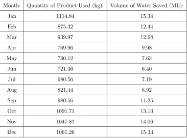
9.5 Volume of water saved by the monolayer for each month of the year and

the quantity of monolayer product used to achieve these savings. . . 186

A.1 Factors that effect a change in water volume (Craig et al. 2005b) . . . . 215

(30)

LIST OF FIGURES xxix

A.3 Schematic diagram showing the structures of the liquid-condensed and

solid monolayer phases. The hydrophilic groups are shown as open cir-cles, and the hydrocarbon (alkyl) chains as grey lines (Barnes 2008) . . 217

A.4 The evaporative reduction performance of three monolayer products

dur-ing trough Trial 6, T1=C18E1; T2=Silicone oil (Aquatain); T3=C16 (WaterSavr at the recommended application rate); T3b=C16 (WaterSavr

at 2x recommended); T4=Control (no monolayer), are presented as the depth deviation from the control. The blue arrow indicate when product

was applied, and the bolder red arrows represent missed applications for C18E1 (Morrison, Gill, Symes, Misra, Craig, Schmidt & Hancock 2008) 223

A.5 Microbial degradation rates of C16OH, C18OH and C18E1 (Pittaway 2008)224

A.6 Surface Pressure vs. Time for ∆−C16OH and O−C18E1. It is

signifi-cant that C18E1 reaches a higher surface pressure in a much shorter time

than C16OH, which indicates that C18E1 spreads more rapidly. Graph reproduced from Deo, Kulkarni, Gharpurey & Biswas (1962) . . . 225

A.7 Floating application units for application of monolayer in a solvent form. (a) Floating solvent application unit. (b) Detailed section of wind valve

for application unit. (c) Floating gear driven water-wheel pump for solvent application. (Treloar 1959) . . . 227

A.8 Underwater gravity-type monolayer film dispenser (Koberg 1969) . . . . 228

A.9 Film pump for producing and spreading a monolayer (Pauken, Jeter & Abdel-Khalik 1996) . . . 230

A.10 Aquatain Dosing Units. (a) DS-1 gravity feed tap-timer system (b) DS-2

peristaltic pumping system . . . 231

(31)

LIST OF FIGURES xxx

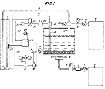
A.12 Oil application, collecting, purifying, controlling and recirculating

sys-tem (Lahav & Alto 1984) . . . 233

A.13 Venturi style emulsion application of molten cetyl alcohol (Reiser 1970) 234

A.14 Wind controlled apparatus for the application of emulsified cetyl alcohol

(Reiser 1970) . . . 234

A.15 Detail of wind controlled valve on the spray heads (Reiser 1970) . . . . 235

A.16 JV-225 boat mounted WaterSavr mixing system (FSI 2007) . . . 236

A.17 WaterSavr mixing system designed and built by Bio-Systems

Engineer-ing (FSI 2007) . . . 237

A.18 Diagram of a Hot-Spray Application System (Florey 1965) . . . 239

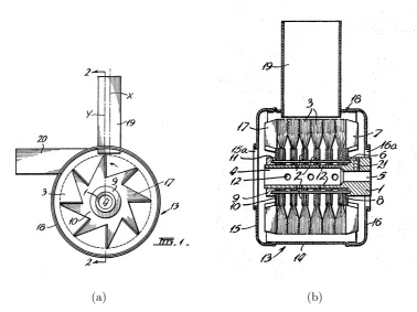
A.19 Diagrams of a Robertson grinder-duster. (a) Detailed internal view (b)

Section along 2-2 (Robertson 1966) . . . 242

A.20 Diagrammatic sketch of the wind operated powder dispensing system. Reproduced from: (Nicholaichuk & Pohjakas 1967) . . . 243

A.21 Nylex pneumatic spreader (Craig 2006) . . . 244

A.22 WaterSavr powder being pneumatically spread from just below the water surface (Brink & Symes 2010) . . . 245

A.23 M-60 Automatic Spreader (FSI 2007) . . . 245

A.24 Prototype temperature differential detection unit (Coop et al. 2008) . . 248

A.25 Comparison of temperature difference between water inside the Y-tube and bulk water outside the tube. Water temperature inside the Y-tube is

(32)

LIST OF FIGURES xxxi

A.26 Water particles at the surface move clockwise on nearly circular paths

as the wave moves from left to right (Cutnell & Johnson 2001) . . . 252

A.27 Relative evaporation and wind speed at various distances from 60% porous slat-fence barrier. Plotted data are averaged from five

obser-vation periods with open-field wind speeds from 6.2 to 7.1m/sec at an elevation of 1.42m above soil surface. Reproduced from (Skidmore &

Hagen 1970) . . . 253

A.28 Relative evaporation and wind speed at indicated distances from 40%

porous slat-fence barrier. Plotted data are averaged from five observation periods with open-field wind speeds from 5.6 to 6.2m/sec at an elevation

of 1.42m. Reproduced from (Skidmore & Hagen 1970) . . . 254

A.29 Relative evaporation and wind speed at various distances from 60% porous slat-fence barrier. Plotted data are averaged from five

obser-vation periods with open-field wind speeds from 6.2 to 7.1m/sec at an elevation of 1.42m above soil surface. Reproduced from (Skidmore &

Hagen 1970) . . . 254

A.30 Crow’s experimental pond showing ’Type B’ closed wind/film barriers

for reducing wind speed and confining monolayer within each bay. Re-produced from (Crow 1963) . . . 256

A.31 Crow’s evaporation reduction tests of wind barriers and baffles with and

without monolayer. (a) The effectiveness of closed wind barriers of dif-ferent spacing/height (L/H) ratios for reducing evaporation. These tests

were made without monolayer. (b) Relative evaporation reduction re-sulting from confinement of C16OH and C18OH fatty alcohol monolayer

(33)

LIST OF FIGURES xxxii

A.32 The effect of a snow-fence windbreak and a monolayer film on cumulative

evaporation. The vertical axis is cumulative evaporation ranging from 0 to 110 cm and the horizontal axis is time ranging from 0 to 170 days.

Reproduced from Nicholaichuk (1978). . . 259

A.33 The effect of a snow-fence windbreak, monolayer film and floating grids on cumulative evaporation. The vertical axis is cumulative evaporation

ranging from 0 to 110 cm and the horizontal axis is time ranging from 0 to 170 days. Reproduced from Nicholaichuk (1978). . . 260

A.34 The wind speed reduction by different shelterbelts. Reproduced from (Naegeli 1953) . . . 261

A.35 Perspective view of Magill’s preferred embodiment of his baffle plate

breakwater (Magill 1953) . . . 264

A.36 Mito’s floating breakwater design. (a) Longitudinal side sectional view

of the elongated floating housing bodies. (b) A plurality of elongated floating housing bodies arranged in parallel to each other. (Mito 1974) . 265

A.37 John O. Olsen’s floating breakwater consisting of a large number of

plas-tic interlocking pontoon modules arrangement (Olsen 1975) . . . 266

A.38 Kodairo and Kunitachi’s floating breakwater design. (a) Plan view of

the floating breakwater. (b) Side view showing a partial cross-section of the floating breakwater (Kodairo & Kunitachi 1976) . . . 267

A.39 Wallace W. Bowley’s floating wave barrier arrangement comprising a

plurality of submerged vessels (Magill 1953) . . . 268

A.40 Perspective view of Angioletti’s floating breakwater and the association of thei device with water waves (Angioletti 1980) . . . 269

A.41 Side view of Kann’s wave suppression system including a plurality of wave suppression members coupled together along a water surface (Kann

(34)

LIST OF FIGURES xxxiii

A.42 Side view, on a greatly enlarged scale, of one end of the devices and a

cross-section of the device showing the internal construction. (Kiefer 1967)270

A.43 End view in cutaway cross-section of Stanwood’s pool lane float (Stanwood 1970) . . . 270

A.44 Side view of a section of one of the racing lane markers and a side view of the racing lane markers arranged with the float means (Walket 1973) 270

A.45 Perspective view of one of the baffle elements and side view of a portion

of the assembly, on an enlarged scale (Walket 1974) . . . 271

A.46 Side view of a cross-section of Lowe’s wave suppression device and a

partial side view of a length of the wave suppression device with portions thereof broken away to show detail (Lowe 1974) . . . 272

A.47 Baker’s wave suppression float member. (a) Cross-sectional view through

the float member. (b) Logitudinal section and a cross-section through a float member (Baker 1977) . . . 273

A.48 Perspective view of a pair of the devices in place on a section of cable

and a typical end elevation of one of the units (Kajlich 1977) . . . 273

A.49 Exploded side view of a fragmentary portion of Rademacher’s lane marker

(Rademacher 1986) . . . 274

A.50 Perspective view of the Kiefer wave suppression element (Kiefer 1990) . 275

A.51 Graphical representation of the energy dissipation efficiency of the present

invention compared to a prior art wave suppression means (Kiefer 1990) 276

A.52 Eddy’s wave suppressor design. (a) Side view of a pair of wave suppres-sors shown as wound around a storage reel. (b) Side view of the wave

(35)

LIST OF FIGURES xxxiv

A.53 A plurality of flexible wave inhibiting devices for a pool lane divider

arranged on a cable (Kajlich 2006) . . . 277

A.54 Diagrammatic view of Ruhlman’s water barrier curtain installed in a body of water. Reproduced from: (Ruhlman 1972) . . . 279

A.55 Thurman’s floating oil containment boom. (a) Side view of a portion of the floating oil containment boom. (b) Front sectional view through the

floating oil containment boom. Reproduced from: Thurman (1973) . . . 280

A.56 Cerasari’s floating oil containment boom. (a) Side elevational view il-lustrating the buoyant support member. (b) Front elevational view of

several buoyant support members. Reproduced from: (Cerasari 1974) . 281

A.57 Fragmental perspective view of the oil fence in a patent by Kinase et al.

(1976) . . . 282

A.58 Isometric view of one individual outrigger-float and frame of the floating barrier. Reproduced from: (Casey 1976) . . . 283

A.59 Geist’s articulated floating oil barrier. (a) Perspective view of an

assem-bled preferred embodiment of the barrier. (b) Plan view in section of a portion of two assembled sections of the barrier. Reproduced from: Geist (1977) . . . 284

A.60 Illustration of a transverse cross-section of this boom at the location of

a stiffener. Reproduced from: Jaffrennou & Cessou (1984) . . . 284

A.61 Smith’s oil containment system for emergency use. (a) Partial cross-sectional view of the oil containment system in its stored position. (b)

(36)

LIST OF FIGURES xxxv

A.62 Vidal’s liquid film maintenance apparatus: (a) Enlarged plan view of

an assembled float member. (b) Perspective view of the various disas-sembled parts of one of the float members. Reproduced from: Vidal

(1967) . . . 286

A.63 Plan view of a typical installation for Vidal’s apparatus. Reproduced from: Vidal (1967) . . . 286

A.64 Plan view of Neilsen’s oil boom fending device. Reproduced from: Nielsen (1977) . . . 287

A.65 Plan view illustrating a mode of use of the fending devices. Reproduced

from: Nielsen (1977) . . . 287

E.1 The design for a centralised monolayer application system. . . 348

E.2 The design for a de-centralised monolayer application system. . . 349

E.3 The design for a hybrid application system, which is a combination of the centralised and de-centralised systems. . . 351

E.4 A concept of a method for applying monolayer as a fine powder ground

from a solid-cast rod using a wire-brush. . . 353

E.5 A variety of other concepts for grinding solid-cast monolayer into a fine powder for application. . . 354

E.6 This is a concept for the application of monolayer from a wax tape. The general idea is that monolayer would be applied to one side of a long

(37)

LIST OF FIGURES xxxvi

E.7 Concept for the spray application of molten monolayer. When the molten

monolayer is sprayed into the air just above the water surface it would solidify into fine particles, which would fall onto the water surface. It

is believed that this form of application would improve the spreading properties of the monolayer. . . 358

E.8 Concept for the application of monolayer as an effervescent tablet. . . . 360

E.9 Concept for the application of monolayer as an effervescent ball/sphere. A sphere shaped tablet would increase surface area over the traditional

disk shaped tablet, thereby enhancing the effervescent reaction upon contact with water. . . 361

E.10 Concept floating monolayer applicator design. . . 363

E.11 Concept design for a low cost adaptation of the current (or similar) CRCIF Floating Applicator for shore-based delivery of monolayer product.365

E.12 A pseudo-sectional view of the simple cantilever anchoring system for

the shore-based monolayer applicator. . . 366

E.13 Pre-prototype floating applicator; (a) three-quarter view of the appli-cator; (b) view underneath the appliappli-cator; (c) view inside the metal housing; and (d) schematic of the anchor and self-adjusting mooring

(38)

List of Tables

1.1 Summary table of three commercially available evaporation mitigation

products evaluated by the NCEA to determine a range (from low to high) for their evaporative reduction performance (%), installation cost ($/m2_{), operating and maintenance cost ($/ha/yr) and breakeven cost}

($/ML saved). Reproduced from Craig et al. (2005b). . . 3

2.1 Comparison of various laboratory studies investigating the relationship between monolayer surface drift speed (Um) and wind speed (Uw). Adapted

from Lange & Huhnerfuss (1978) and Hale & Mitchell (1997). . . 21

2.2 Comparison of the various UM AX values (wind speed cut-off point for

monolayer application) adopted by researchers during field trials. . . 22

2.3 Fractional loss of monolayer material from a monolayer film at a surface pressure of 35mN/m. Adapted from Brooks & Alexander (1960). . . 23

2.4 Summary of relevant information from field studies employing distributed

application systems for monolayer in a liquid form. . . 34

5.1 Surface pressures measured for C18OH and Brij78 in water-emulsion at

(39)

LIST OF TABLES xxxviii

5.2 Summary of monolayer quantities applied and water temperatures

dur-ing testdur-ing, includdur-ing the constants and exponents derived from the 0.3, 2 and 6 m diameter tank results. . . 77

6.1 Comparison of various laboratory studies investigating the relationship

between clean water surface drift speed (us) and wind speed (uw). Field

studies in lakes and open oceans have been omitted from this table as us is generally greater, most likely due to an increase in Stokes mass

transport by developed deep-water waves (Lange & Huhnerfuss 1978). Adapted from (Lange & Huhnerfuss 1978) and (Hale & Mitchell 1997). . 86

6.2 Summary of the drift velocity test application rates used for each

refer-ence wind velocity. . . 101

6.3 Summary of the spread angle test application rates used for each refer-ence wind velocity. . . 107

7.1 Table as output from the MATLAB simulation platform showing the Cartesian coordinates (x and y location) of each applicator and the

corresponding total amount of monolayer applied for that applicator. Applicator locations are listed anti-clockwise, starting from the bottom

left-hand corner of the distribution graph (Figure 7.5). . . 134

8.1 BOM wind rose speed ranges and the corresponding wind speeds used

in modelling. . . 141

8.2 Percentage of time a minimum area is covered for the 50 x 50 m storage after 1 hour of application. Including the average of the percentages

of time, the aggregate application rate over that period and the total amount of monolayer applied for each arrangement. Results calculated

(40)

LIST OF TABLES xxxix

8.3 Percentage of time a minimum area is covered for the 500 x 500 m storage

after 3 hours of application. Including the average of the percentages of time, the aggregate application rate over that period and the total

amount of monolayer applied for each arrangement. Results calculated using BOM average annual wind speeds and directions for both Amberley

and Moree. . . 156

8.4 Percentage of time a minimum area is covered for the 5000 x 5000 m storage after 5 hours of application. Including the average of the

per-centages of time, the aggregate application rate over that period and the total amount of monolayer applied for each arrangement. Results cal-culated using BOM average annual wind speeds and directions for both

Amberley and Moree. . . 159

8.5 Percentage of time a minimum area is covered for the 500 x 500 m storage after 3 and 6 hours, the average of the percentages of time, the aggregate

application rate over that period and the total amount of monolayer applied for each arrangement. Results calculated for Moree only. . . 161

9.1 Decision table capturing the water quality attributes of three water stor-ages in south-east Queensland (Pittaway & van den Ancker 2010) were

matched with the performance specifications of three monolayer com-pounds to predict which product will best perform on a given storage. . 170

9.2 Data output from the simulation platform, which details the percentage

of cover achieved, the aggregate application rate and the time to steady-state for each wind condition. . . 181

9.3 Data output from Post-Process 1 using the percentages of cover for each

wind condition, as output from the simulation platform (Table 9.2), and applying a weighting for the frequency of that wind condition occur-ring. The frequency weightings were derived from BOM wind speed and

(41)

LIST OF TABLES xl

9.4 Data required for Post-Process 2. These data were determined via the

simulation platform and Post-Process 1 using monthly wind speed and direction frequency data from the BOM for Amberley, Qld. Simulations

were run firstly for all applicators, and secondly for the shore-based applicators only. . . 185

9.5 Data output from Post-Process 2 detailing the monthly quantity of

mono-layer product used and the volume of water saved. . . 187

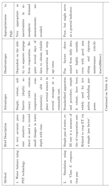
A.1 Summary of the advantages and disadvantages of various methods for

measuring evaporation from farm water storages (Part 1). Overview based on Craig and (Hancock 2008) . . . 210

measuring evaporation from farm water storages (Part 2). Overview based on Craig and (Hancock 2008) . . . 211

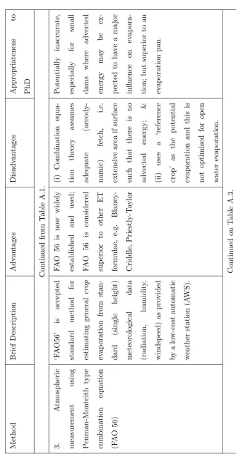
A.3 Summary of the advantages and disadvantages of various methods for measuring evaporation from farm water storages (Part 3). Overview

based on Craig and (Hancock 2008) . . . 212

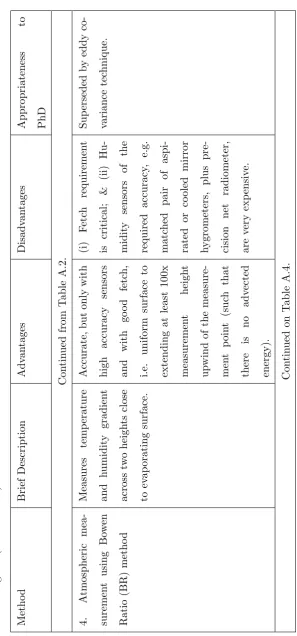
A.4 Summary of the advantages and disadvantages of various methods for measuring evaporation from farm water storages continued (Part 4).

Overview based on Craig and (Hancock 2008) . . . 213

measuring evaporation from farm water storages continued (Part 5). Overview based on Craig and (Hancock 2008) . . . 214

A.6 Commercially produced chemical film products currently available in

(42)

LIST OF TABLES xli

A.7 Mean wind speed reduction in the lee of four different density

shelter-belts over distances of 10H, 20H and 30H. H is the distance (down wind) from the shelterbelt where the wind speed measurement was taken.

Re-produced from (Naegeli 1953) . . . 262

C.1 Amberley average annual (9am and 3pm) wind frequency table used in modelling (Part 1). . . 300

C.2 Amberley average annual (9am and 3pm) wind frequency table used in modelling, continued (Part 2). . . 301

C.3 Moree average annual (9am and 3pm) wind frequency table used in

mod-elling (Part 1). . . 306

C.4 Moree average annual (9am and 3pm) wind frequency table used in

mod-elling, continued (Part 2). . . 307

D.1 Decision table A (Part 1). . . 309

(43)

LIST OF TABLES xlii

D.20 Decision table B (Part 1). . . 328

(44)

LIST OF TABLES xliii

(45)

(46)

LIST OF TABLES xlv

Acronyms & Abbreviations

˚

A Angstrom (=10−10m) ˚

A2 Square angstrom (=10−20m2) ABS Australian Bureau of Statistics BOM Bureau of Meteorology (Australia)

C12OH Dodecyl or lauryl alcohol or dodecanol (C12H26O)

C14OH Myristyl alcohol or tetradecanol (C14H30O)

C16OH Cetyl alcohol or hexadecanol (C16H34O)

C18OH Stearyl alcohol or octadecanol (C18H38O)

C20OH Arachidyl alcohol or icosanol (C20H42O)

C18E1 Ethylene glycol monooctadecyl ether (C20H42O2)

CRC-IF Cooperative Centre for Irrigation Futures

CSIRO Commonwealth Scientific and Industrial Research Organisation

ERF Evaporation reduction factor GL Gigalitre (=109L)

ML Megalitre (=106L)

NCEA National Centre for Engineering in Agriculture

SEQ South East Queensland

SGS Sociètè Gènèrale de Surveillance UDF Universal Design Framework

Um/Uw Ratio of monolayer surface drift speed and wind speed

UM IN Minimum wind speed threshold

UM AX Maximum wind speed threshold

UNE University of New England

(47)

Chapter 1

Introduction

1.1

Background

The following section provides an introduction to the Australian agricultural context,

estimates of water loss from farm water storages due to evaporation and available technologies to farmers to mitigate these losses. Further detail with respect to using a

chemical monolayer1 to protect open water surfaces is also provided.

1.1.1 Context

Australia is the driest inhabited continent on the Earth. It is a continent of climatic extremes, experiencing great variations in rainfall and evaporation, according to region

and season. Rainfall is generally confined to a narrow strip along the north and east coast of the continent, including Tasmania (BOM 2007). Australia’s often hot

tem-peratures, dry air and strong winds means that water evaporates into the atmosphere at high rates. On average 92% of rainfall is re-evaporated, 7% reaches the sea and

1% recharges aquifers (ABS 2004). Seventy per cent of the country experiences mean monthly potential evaporation greater than its mean monthly rainfall, and for nearly

(48)

1.1 Background 2

(Fietz 1970).

Annual evaporation losses from farm water storages in Australia can potentially exceed

40% of storage volume (Craig et al. 2005a). While the extent and distribution of farm water storages is not accurately known, it is conservatively estimated that nationally

there is in excess of 12,500 GL of water stored on an estimated 22,000 agricultural enterprises. There are also approximately 500 registered large dams across Australia

representing a further 85,000 GL of water. In addition, considerable water distribution losses are present in irrigation channels due to evaporation and seepage.

Although it is hard to accurately estimate Australia’s total evaporative water loss, it is probable that thousands of GLs of water are lost each year from water storages.

As a consequence, production opportunities worth tens of millions of dollars evaporate with the water. The outlook for the future is no better with the effects of climate

change predicted to increase average temperatures across Australia, which will seriously affect evaporation and the viability of our current land use. It is predicted that by

2030 most of Australia will experience an annual warming of between 0.4◦C and 2◦C relative to 1990, and by 2070, temperatures are estimated to rise between 1◦C and 6◦C

(CSIRO 2008).

Evaporation losses from storages can be minimised to some extent during design and construction through deep, small surface area storages or construction of storages with cells. Also the use of wind barriers, shelter belts and even dam destratification can

help to reduce evaporative loss. Beyond this there are commercially available products such as floating covers (E-VapCap), suspended shade structures (NetPro) and chemical

additives (WaterSavr).

The National Centre for Engineering in Agriculture (NCEA), which has been work-ing actively in the field of evaporation mitigation for a number of years, conducted

large scale engineering assessments of the three evaporation mitigation technologies noted above (Craig et al. 2005b). Table 1.1 summarises the product performance and

breakeven costs of these products.

(49)

1.1 Background 3

cost of water saved ($130/ML at 30% efficiency). In addition, chemical monolayers

need only be applied when water is in storage or when evaporation rates are high. This can reduce cost ($/ML) to 75% of that shown in Table 1.1 when for example water is

only held in storage between October and March (expected period of high evaporation). Further savings can also be achieved by more judicious monolayer application strategies.

1.1.2 Using a chemical monolayer to protect open water surfaces

Monolayers are not a new technology; in 1925 it was shown that the application of

monomolecular films of certain organic compounds to a water surface can decrease the rate of evaporation (Frenkiel 1965). Following this discovery there were intensive

laboratory studies, but it was not until 1952, in Australia, that the first attempts were made to apply monolayer under natural conditions to open water surfaces to

reduce evaporation (Mansfield 1955). Subsequently many investigations have followed in Australia: Treloar (1959), Vines (1960a), Robertson (1966); in United States of

America: Dressler & Guinat (1973), Crow (1963), Florey (1965), Reiser (1969), Koberg (1969); in Canada: Nicholaichuk (1978); in India: Walter (1963) and in Israel: Lahav

Table 1.1: Summary table of three commercially available evaporation mitigation products

evaluated by the NCEA to determine a range (from low to high) for their evaporative

reduc-tion performance (%), installareduc-tion cost ($/m2_{), operating and maintenance cost (}_$_/ha/yr)

and breakeven cost ($/ML saved). Reproduced from Craig et al. (2005b).

Product Evaporation Reduction (%) Installation Operating Breakeven

Small Tank Farm Dam Cost Cost Cost

(measured) (estimate) ($/m2) ($/ha/yr) ($/ML saved)

E-VapCap 94%-100% 85%-95% $5.50-$8.50 $112-$572 $302-$338

NetPro 69%-71% 60%-80% $7.00-$10.00 $112-$537 $296-$395

(50)

1.1 Background 4

& Alto (1984). A full review of these studies is provided in Appendix A.

Although chemical monolayers offer great potential, their evaporation reduction

perfor-mance has been shown to be highly variable and is affected by a number of influencing factors; in particular wind and wave action. In field studies at Lake Hefner, U.S.

Bu-reau of Reclamation researchers found wind to be the single most important factor in the application and maintenance of monolayer film (Fietz 1959). Subsequently several

strategic approaches were employed to reduce or eliminate the adverse effects of wind. They include: (1) continuous replenishment of monolayer at the up-wind shore, (2)

re-duction of wind speed near the water surface by wind-breaks along the shore or floating on the surface, and (3) restriction of air and film movement by confinement within a network of floating compartments.

The three strategies noted above were trialled at the Oklahoma Agricultural

Experi-mental station (Crow 1963). At the conclusion of the trial, Crow noted that the method of continuous application of monolayer is the only feasible approach to the wind

prob-lem on large reservoirs. Alternatively, approaches 2 and 3 only offer an economical means of reducing evaporation losses from small farm storages.

Currently the bulk of research and development into evaporation mitigation by

mono-layers is being undertaken by the NCEA within their ‘Dam Evaporation Mitigation’ project, which was funded by the Cooperative Research Centre for Irrigation Futures (CRC-IF)2_{. Also collaborating with the NCEA through the CRC-IF is a group at the}

University of New England (UNE) who are developing sensing technologies for detect-ing the presence of a monolayer film on the water surface. These sensdetect-ing technologies

are particularly relevant to this project and are fundamental in determining monolayer spatial distribution, breakdown and overall performance.

2

Although the CRC-IF ended its 7 year term on June 30, 2010 this following link serves as an archive

(51)

1.2 Hypothesis and research aim and objectives 5

1.2

Hypothesis and research aim and objectives

1.2.1 Hypothesis

The central hypothesis of this research is:

i. that present application systems and application strategies for applying chemical

monolayer materials to open water surfaces are sub-optimal which has a deleteri-ous effect on the spread and formation of an effective cover, which in turn results

in an inconsistent and usually poor evaporation reduction performance; and

ii. that significant improvements in monolayer performance maybe achieved through:

– developing a better understanding of factors that influence monolayer per-formance and the environmental range/boundaries for the effective use of

monolayer, then

– utilise this information for the design, installation and operation of an au-tomated monolayer application system, which is tailored to site-specific en-vironmental conditions and user requirements.

1.2.2 Research aim and objectives

The aim of this research is to formulate and develop a universal framework to inform

the selection of suitable monolayer material/s, the design of the application system and the application strategies to be used for a specific site. As every user and site

is likely to be different, the framework developed will need to be robust enough to handle the differing site conditions and user requirements. It is anticipated that this universal framework will help to optimise the evaporation suppressing performance of

the selected monolayer.

The aim to develop a Universal Design Framework (UDF) has led to the following research objectives and associated tasks:

(52)

1.2 Hypothesis and research aim and objectives 6

• Identify environmental conditions that effectively nullify monolayer performance.

These conditions will form the working environmental range/boundaries for mono-layer use as well as the UDF.

• Identify influencing factors that will need to be taken into consideration for the

design, planning, installation and operation/management of the application sys-tem.

• Identify the UDF information and processing requirements needed in order to

de-termine suitable monolayer material/s, application system design and application strategies for a particular storage and user requirements.

• Formulate a UDF that incorporates all of the important influencing factors,

en-vironmental boundaries and processing requirements identified.

Objective 2 - Large-scale laboratory study of monolayer dispersion charac-teristics:

• Identify an existing evaporation suppressing monolayer material and develop a

form in which the material can easily be used for all empirical work and for possible future field trials.

• Characterise the spreading rate and spreading pattern of monolayer for calm wind

conditions when non-continuous application would be required.

• Characterise drift rate, spreading rate and spreading pattern for a range of wind conditions when continuous application would be required.

• Derive algorithms from the above empirical work for calibration of the simulation

platform.

Objective 3 - Simulation platform development and demonstration:

• Develop a basic simulation platform capable of estimating/predicting monolayer

(53)

1.3 Overview of dissertation 7

• Calibrate the model with the algorithms derived from the laboratory study of

monolayer dispersion characteristics.

• Demonstrate the ability and robustness of the simulation platform in modelling the distribution of monolayer for different wind conditions, storage sizes and

ap-plication periods.

Objective 4 - Scope and demonstration of the UDF:

• Create a decision table that will allow the user to make numerical comparisons

between the South East Queensland (SEQ) benchmark reservoirs and their own to determine the most suitable monolayer compound/s for their storage.

• Develop a process for using the UDF to determine a customised applicator

ar-rangement with the simulation platform.

• Demonstrate the ability of the UDF for determining suitable monolayer

produc-t/s, optimal application system, decision tables for real-time application and the

expected performance of the application system.

1.3

Overview of dissertation

(54)

Figure

1.1:

Blo

ck

diagram

of

dissertation

o

v

(55)

• Chapter 2provides a literature and scientific review of many different specialty areas within chemistry, physics and biology relating to the use of a monolayer for evaporation mitigation on agricultural water storages. Much of this

infor-mation is largely summarised from Appendix A. Through the literature review the fundamental gaps in knowledge were identified, which also help