THE DEVELOPMENT OF A DUCTED WIND TURBINE SIMULATION MODEL
Andy Grant, Nick Kelly
Energy Systems Research Unit, University of Strathclyde, Scotland
e-mail: [email protected], [email protected]
Tel: +44 (0)141 548 3986 Fax: +44 (0)141 552 5105
ABSTRACT
Embedded generation has been described as a “paradigm shift” in the way in which electricity is produced, with the focus of power production shifting away from large centralised generation plants to production of heat and power close to the point of use.
An emerging technology that may play a part in the evolution of this new paradigm is the ducted wind turbine (DWT). Up to this point, wind energy has not played a major role in embedded generation for the built environment. However, the development of these small micro turbines that can be integrated into the building fabric, opens up the possibility of utilising the differential pressures that occur due to airflow around buildings for the purpose of local power production.
This paper describes recent work to develop and test a simple mathematical model of a Ducted Wind Turbine and its integration within the various technical domains of a building simulation tool. Specifically, the paper will describe: a) the concept of the ducted wind turbine; b) the development of the mathematical model; c) the integration of the model into a building simulation tool.
The paper will conclude with a case study in which the simulation model will be used to analyse of the likely power output from a building design incorporating ducted wind turbines within the facade.
Keywords: ducted wind turbine, mathematical model, embedded generation, building simulation.
INTRODUCTION
As we move into the 21st century technological innovation is changing the means by which heat and power can be delivered to the built environment. New “micro-grid” type technologies offer the potential of supplying heat and power locally from “clean” and energy- efficient-type technologies. Examples of these technologies include micro-CHP
using Stirling engines, photovoltaics (PV) and fuel cells.
To assess the effectiveness of these devices and also to assess the impact of their diffusion into the built environment it is necessary to develop models to simulate their performance in a realistic operational context. Building simulation offers a means to do this and can reveal important performance characteristics such as the total energy yield, the temporal characteristics of heat and power output and their compatibility with the loads that they are designed to serve.
The ducted wind turbine (DWT) (Webster, 1979) is an emerging micro-grid technology; this is a small, wind energy conversion device that can be integrated into the façade of a building and may be a useful means of producing power in areas with windier climates. The ducted wind turbine overcomes many of the problems associated with the use of conventional wind turbines in an urban environment, which are hampered by high levels of turbulence in the air stream, and are also constrained by concerns over visual impact, noise and public safety. In contrast DWT units are purposely designed for attachment to buildings and are both robust and unobtrusive.
This paper describes the integration of a simple DWT model (Grant et al. 2002) into a building simulation tool.
THE DWT MODEL
The model described here has been derived from a design (figure 1) that attaches to the roof edge of rectangular-section buildings, making use of the pressure differentials that are naturally created by the action of the wind.
To illustrate the potential for power production from such a device, a simple, validated mathematical model has been constructed for one-dimensional flow (Grant et al. 2002). This is shown in Figure 2.
Eighth International IBPSA Conference
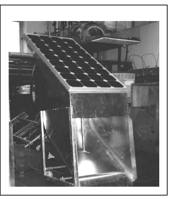
Figure 1 a picture of a DWT.
Analysis of this model shows that the power extracted from the air stream is:
−
= ∞
2 2 2 2
2
2
2 v
T
C U U U A
W ρ δ (1)
Differentiating Equation 1 with respect to U2 gives
the maximum power condition:
∞
=
C
U
U
v.
3
2δ
(2)Substituting this into Equation 1 gives the maximum power output:
3 2 3
max
3
3
∞=
C
A
U
W
vT
ρ
δ
(3)1. 2.
v8
v2
ÄPT WT
Figure 2 a simple model of a ducted wind energy conversion device.
The power output of the component is therefore a function of the duct velocity coefficient (Cv), the
opening area A and the free stream velocity of the wind, U∞. Experimental analysis (Grant et al. 2002) has shown Cv to be close to 1.0
Equation 3 can be re-arranged to give the power output in terms of a power coefficient CP and the
available power in the wind Pw, which is defined as:
3
2
1
∞
=
A
U
P
wρ
(4)By inspection of Equation 3 the power coefficient is:
2 / 3
3
3
2
δ
v
p
C
[image:2.595.312.512.236.457.2]C
=
(5)Figure 3 the variation of CP with ä.
And the power extracted from the air stream is:
w p
T
C
P
W
max=
(6)Figure 3 shows the variation in CP with the pressure
coefficient differential across the turbine.
In conventional wind turbines the power coefficient peaks around 0.593 (the Betz limit). However it is clear from Figure 3 that power coefficients considerably greater than the Betz limit are obtainable for ducted wind turbines if losses in the duct are kept to a reasonable minimum.
The reason for this is that the achievable pressure differential across the DWT, ÄP, is far higher than that achievable with a conventional wind turbine. This is due to the fact that for the DWT the ÄP is being created by the air flow over the building, whereas in a conventional turbine the ÄP is caused by the air flow through the blades themselves.
U
U
2Variation of Cp with
0 0.2 0.4 0.6 0.8 1 1.2 1.4 1.6
0 0.5 1 1.5 2 2.5
Cp
δ δ
[image:2.595.71.269.501.721.2]INTEGRATION WITH BUILDING
SIMULATION
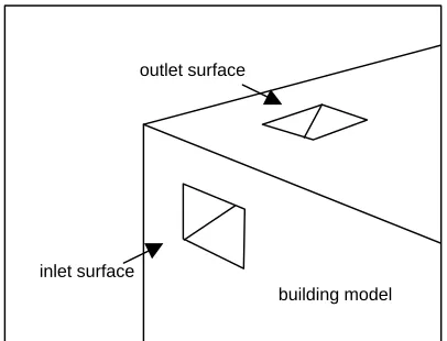
Equation 3 forms the basis of the DWT model that has been integrated into the ESP-r building simulation tool as a building-integrated renewable energy component. Examples of other renewable components that already exist in the tool include solar collectors and photovoltaics. These components utilise boundary condition data provided by ESP-r (solar radiation, temperature, etc.) to calculate their heat and/or power output. They are fully integrated with the rest of the building model. For example the PV model is defined as a component of the building fabric, which interacts with both the thermal and electrical domains of an ESP-r model (Kelly et al 2001).
In a similar fashion, to calculate its power output, the DWT model uses the wind velocity and direction, and ESP-r’s calculation of inlet and outlet surface pressure coefficients
i
δ
ando
δ
respectively.These pressure coefficients and their differential
δ
(used in equations 1,2,3 and 5) are derived from the pressure difference, ÄP, (based on stagnation pressures) across the inlet and outlet surfaces of the DWT:(
2 2)
2
1
∞
∞
−
=
∆
P
δ
iρ
U
δ
oρ
U
(7)The differential pressure coefficient is therefore:
o
i
δ
δ
δ
=
−
(8)It follows that the pressure difference across the DWT can be found from:
2
2
1
∞
=
∆
P
δρ
U
(9)ESP-r can calculate values of
δ
i andδ
o and supplythem to the DWT model so that
δ
can be calculated. To achieve this the DWT component is linked to two surfaces on the ESP-r building model (figure 4). At any time t during a simulation ESP-r’s calculated values ofδ
i andδ
o for these surfaces, and the valueof the free stream wind velocity, U
∞, held in the
[image:3.595.317.520.100.255.2]simulation climate file are fed into the DWT model. This then calculates the instantaneous electrical power output (W).
Figure 4 integration of the DWT model into a building model.
CLIMATE DATA
The output of all of ESP-r’s renewable energy components is heavily influenced by the climate data that provides the boundary conditions for their solution. ESP-r simulations generally use hourly averaged climate data. In the case of the solar energy components (PV and solar thermal collectors) the output is largely a linear function of the solar intensity falling on the component and so the use of the use of averaged data is not a problem.
In the case of the DWT model the power output is influenced by the local wind speed and direction and power output is a function of the cube of the incident free stream wind speed. So the model will be particularly sensitive to higher speeds, which have a disproportionate impact on the power output. Around buildings in the urban environment such high speeds frequently occur in short duration “gusts”.
Gusting is a manifestation of the high levels of turbulence, e.g. over 30% turbulent intensity (Feranec et al. 2001), found in the so-called “urban canopy”. High turbulence levels lead to significant, high-frequency changes in both wind direction and speed.
As mentioned, the data used in building simulation tools is usually time-averaged, hourly data, often collected at rural weather stations, where the local microclimate and characteristics of the atmospheric boundary layer are often very different to that found in urban areas. This is problematic for the DWT model. Firstly, the use of time-averaged data will filter out effects such as wind gusting, which will impact on the power output calculations of the model. Secondly, the wind speed data is often recorded at a different height to that which DWTs may be located on a building. Consequently, direct
inlet surface
outlet surface
use of “raw” climate data as read from a simulation climate file may give misleading results as to the potential for power output from the DWT device1.
Various techniques have been developed to overcome these problems. The effect of height differences between the measurement point and the location of a simulation component on the wind velocity is often addressed by adjusting the measured data according to an assumed wind velocity profile. An example is the power law profile (Liddament, 1986):
a l
l
Kz
U
U
=
10
(10)
However, profiles must be applied with caution, particularly in urban environments, where their use is often inappropriate, as wind patterns at within the urban canopy may be dominated by neighbouring buildings.
The use of CFD is a useful means of gauging the impact of surrounding buildings (including the building itself) on the local airflow direction and speeds in relation to the prevailing direction and speed. (Danneker 2001) has used CFD to generate the local wind speeds and pressure coefficient differentials required by the DWT model for a particular building.
To overcome the filtering out of short-duration changes in wind speed and direction the DWT model has been equipped with an efficient statistical model, which takes the averaged free stream wind speed and direction in the climate file and an assumed value of the local turbulent intensity to calculate a distribution of wind speed and direction about their mean values; this distribution is then used by the DWT model to calculate power output over the simulation time step.
Note that this statistical approach does not give a picture of the short-term temporal variation in power output as would be provided by the use of high-frequency monitored wind data with the model. The use of such data would be necessary if the model was used in power quality analysis.
1
It should also be noted that the arguments put forward here relating to hourly averaged wind data also apply to infiltration models.
To calculate the distribution of wind speeds and the wind directions about their mean values the two readings [
U
∞,
θ
] are recast into two component velocities:θ
sin
∞
=
U
u
(11b)θ
cos
∞=
U
v
(11b)The instantaneous values of these two components is given by
u
u
u
=
+
′
(12a)v
v
v
=
+
′
(12b)Where the barred values are the components of mean wind speed and the dashed components are the fluctuating velocity2. The instantaneous values of the two components are assumed to follow a normal distribution about the mean speed, which can be described using the following standard probability density function:
−
−
=
2
2
1
exp
2
1
)
(
u u
u
u
u
σ
π
σ
f
(13)
The standard deviation, ó, can be expressed in terms of the turbulent intensity (I) of the air flow. Turbulent intensity is defined as (Schlichting, 1968):
∞
′
+
′
+
′
=
U
z
v
u
I
3
2 2
2 (14)
Now in turbulent flow the root mean squared value of fluctuations in all directions are assumed to be identical so that the turbulent intensity can be expressed as:
2
∞ ∞ = ∞
≅
−
=
′
=
∑
U
U
n
U
I
n i uu
u
u
2 1σ
)
(
1
(15)
Where n is the number of readings of a particular velocity component u (u = u, v or w) over a period of time. Equation 12 is valid if n is large. The standard deviation of the velocity component u can therefore be re-expressed in terms of the turbulent intensity I and the free stream velocity:
∞
=
I
U
uσ
(13)The probability density function for each velocity component can therefore be re-written in terms of the turbulent intensity and the free stream velocity.
−
−
=
∞ ∞ 22
1
exp
2
1
)
(
U
I
U
I
f
u
u
u
π
(16)The actual probability of wind speeds occurring over a range [a,b] is given by:
∫
= ==
b ad
f
p
u uu
u
)
(
(16)The effect of changing the turbulent intensity of the air flow in Equation 14 is shown in figure 5. Increasing I increases the spread of velocities and reduces the height of the probability density curve at the mean wind speed.
Equation 11 is embedded in the DWT model. At each simulation time step the model makes n samples and calculates the probability density and then probabilities of a range of u and v values, and the combinatorial probabilities of [u,v] pairs.
The range of velocities explored about the mean is A 3-D distribution of the time duration for a range of wind speeds and directions can then be developed for each time step based on the turbulent intensity. The time duration of each [u,v] pair is given by:
t
v
u
p
t
u,v=
(
,
)
×
∆
(16)Where p(u,v) is the probability for the particular instance of u and v occurring together. Ät is the
simulation time step length. The wind velocity components u and v are then re-cast as a speed and direction (Ui,èi), and these, together with their time
duration and ESP-r’s calculation of the pressure coefficient differential associated with (Ui,èi), ä(Ui,èi),
[image:5.595.74.271.75.130.2]can then be passed to Equation 3 to calculate the turbine energy output for that particular combination of u and v. The average power output of the turbine over the time step is the sum of the energy calculations for each [u,v] pair divided by the simulation time step length.
Figure 5 the effect of changing I in Equation 11
CASE STUDY
This case study illustrates the use of the DWT model within the ESP-r building simulation tool and also highlights some of the issues raised in relation to the use of averaged climate data sets with the model.
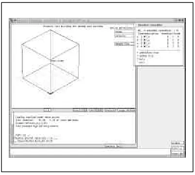
Figure 6 shows a very simple building model with which the DWT model is used. The building has a floor area of 100m2, is 10m high and assumed to be located in a city centre, hence the surfaces for which
δ is calculated (using values from ESP-r’s pressure coefficients database) are assumed to be semi-sheltered. A total of eighty ducted DWTs are attached to the North, South, East and West facades of the building. Each turbine has an inlet face area of 0.2m2 and a cut-in wind speed of 4ms-1.
In these simulations the power output of the ducted wind turbines is calculated over the course of a year using the UK average climate data set. Five simulations were run to illustrate the effects of wind speed averaging, the statistical wind speed data manipulation described previously and turbulent intensity on the performance of the DWT model. It is assumed that In the first simulation the only the
Probability Density Umean=5
-0.20 0.00 0.20 0.40 0.60 0.80 1.00 1.20 1.40 1.60 1.80
-5 0 5 10 15
Wind Velocity Probability Density I=5% I=10% I=25% I=50% . 3
3 = ± ∞
± u IU
[image:5.595.303.529.232.425.2]hourly averaged data values held in the climate file are used. In the following simulations, the wind speed data is manipulated using the statistical method described with turbulent intensities of 5, 10, 20 and 30% respectively. These turbulent intensities can be regarded as ranging from high (30%) to low values (5%).
Figure 7 shows the power output from the simulations. Clearly there are considerable differences in these predictions, with simulations 2, 3 4 and 5 producing 0.5%, 6%, 26% and 60% more electrical energy output respectively than simulation 1, illustrating the effect of the statistical model and particularly the value of turbulent intensity (I). This is seen to have a critical impact on the predictions of power output from the model with simulation 5 (I=30%) predicting 59% more electrical production than simulation 2 with I=5%.
Figure 8 shows the impact of the different simulations on the total power output from the turbines over the course of the simulation period. The statistical manipulation of the wind speed slightly increases the occurrence of high power outputs, while slightly reducing the occurrence of low power outputs. This effect increases with the value of turbulence intensity and is as would be expected: a high turbulent intensity increases the likelihood of higher velocity gusts while reducing the occurrence of wind speeds at the mean.
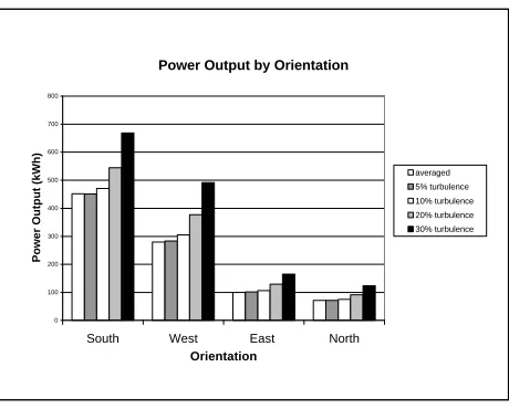
Figure 9 shows the contribution of the different facades of the building to the total electrical energy production. The prevalent wind direction is approximately from the south-west, so the bulk of the
power produced is from the south and west facade. This pattern is unaffected in the five simulations.
Figure 6 a simple building model.
Analysis has shown that the generator attached to the DWT has an efficiency of around 65% over a range of rotational speeds (Ewen, 1999). Using this value, the average energy yield predicted for the DWT components is around 55-90 kWh/m2, the higher power outputs occurring with greater turbulent intensity. This compares favourably with a typical value of 30-40 kWh/m2 from photovoltaics (PV) in the same climate (Clarke et al. 2000) and illustrates that ducted wind turbine devices are a viable alternative to photovoltaic facades in areas with a reasonable wind resource and lower levels of sunshine.
Total Power Output
0 200 400 600 800 1000 1200 1400 1600
Power Output (kWh)
averaged 5% turbulence 10% turbulence 20% turbulence 30% turbulence
Power Output Frequency of Occurrence
1 10 100 1000 10000
0 500 1000 1500 2000 Total Power Output (W)
Frequency
averaged 5% turbulence 10% turbulence 20% turbulence 30% turbulence
[image:6.595.71.516.336.523.2]Figure 9 the contributions from the different facades to power production.
CONCLUSIONS
This paper has outlined the basis for a simple ducted wind turbine (DWT) model and demonstrated how it has been integrated into the ESP-r building simulation tool.
The model is sensitive to wind speed and a statistical technique using the wind turbulent intensity is employed to account for the effect of short duration, high velocity wind gusts on the power output. This effect that would otherwise be lost using hourly averaged data.
Several simulations were conducted and showed that accounting for gust effects leads to a significant increase in power output predictions from the model.
The simulated average energy yield compares favorably to that of photovoltaic materials, indicating that the ducted wind turbine shows potential as a micro-grid power source and deserves much more investigation.
REFERENCES
Clarke J A, Johnstone C M, Macdonald I A, French P, Gillan S, Glover C, Tatton D, Devlin J and Mann R, 2000, The deployment of photovoltaic components within the lighthouse building in Glasgow, Proc. 16th European Photovoltaic Solar Energy Conference, Glasgow.
Danneker R, 2001, Wind energy in the built environment: an experimental and numerical investigation of a building integrated ducted
wind tubine module, PhD Thesis, University of Strathclyde, Glasgow.
Ewen Stuart, 1999, Analysis of a vertical axis ducted wind turbine, BEng Thesis, University of Strathclyde Glasgow.
Feranec T, Feranec V, 2001, Wind load on buildings and structures in groups, Proc. 39th International Conference in Experimental Stress analysis, Czech Republic.
Grant, A D, Dannecker, R K and Nicolson, C D, 2002, Development of building-integrated wind turbines. Proc. World Wind Energy Conference, Berlin.
Kelly N J, Clarke J A, 2001, Integrating power flow modelling with building simulation Energy and Buildings 33(4) pp333-40.
Liddament M W, 1986, Air infiltration calculation techniques - an applications guide, IEA Air Infiltration And Ventilation Centre (AIVC), Bracknell (UK).
Schlichting H, 1968, Boundary layer theory, McGraw Hill, 6th Ed.
Webster G W, 1979, Devices for utilising the power of the wind, USA Patent No. 4154556.
NOMENCLATURE
a,K coefficients for calculation of wind speed from a profile
-A duct area m2
Cv duct velocity coefficient
-I Turbulence intensity %
PW Power contained in the wind W
P(u,v) probability of velocity
components[u,v] occurring in a simulation time step
%
n number of samples in a time step
-t,Ät time, timestep length s
u,v velocity components m/s
v
u
,
Average velocity components m/sv
u
′
,
′
fluctuating velocity components m/sz ,zl velocity component, height
u general velocity component m/s
U ,Ul free stream wind speed, wind
speed at height l
m/s Power Output by Orientation
0 100 200 300 400 500 600 700 800
South West East North Orientation
Power Output (kWh)
U10 measured wind speed m/s
WT work extracted by turbine W
ä pressure coefficient differential
-è wind direction o
ñ density kg/m3