Acceptor splice site prediction

Rochester Institute of Technology

RIT Scholar Works

Theses Thesis/Dissertation Collections

5-1-2007

Acceptor splice site prediction

Eric Foster

Follow this and additional works at:http://scholarworks.rit.edu/theses

This Thesis is brought to you for free and open access by the Thesis/Dissertation Collections at RIT Scholar Works. It has been accepted for inclusion in Theses by an authorized administrator of RIT Scholar Works. For more information, please [email protected].

Recommended Citation

THESIS

ACCEPTOR SPLICE SITE PREDICTION

by

Eric Foster

Submitted in partial fulfillment of the requirements for the

Master of Science degree

In

Bioinformatics

at

ii

THESIS ADVISORY COMMITTEE

1. Committee Advisor

Dr. Shuba Gopal

Assistant Professor

Department of Biological Sciences College of Science

Rochester Institute of Technology

2. Committee Advisor

Dr. James Halavin

Professor

School of Mathematical Sciences College of Science

Rochester Institute of Technology

3. Committee Member

Dr. David Lawlor

Associate Professor

Department of Biological Sciences College of Science

Rochester Institute of Technology

4. Committee Member

Dr. Gary Skuse

Associate Professor

Department of Biological Sciences College of Science

iii

Thesis Author Permission Statement

Title of thesis: _______Acceptor Splice Site Prediction ________________

Name of author:____ Eric D. Foster ____

Degree: Master of Science

Program: Bioinformatics

College: Science

I understand that I must submit a print copy of my thesis or dissertation to the RIT Archives, per current RIT guidelines for the completion of my degree. I hereby grant to the Rochester Institute of Technology and its agents the non-exclusive license to archive and make accessible my thesis or dissertation in whole or in part in all forms of media in perpetuity. I retain all other ownership rights to the copyright of the thesis or dissertation. I also retain the right to use in future works (such as articles or books) all or part of this thesis or dissertation.

Print Reproduction Permission Granted:

I, Eric D. Foster , hereby grant permission to the Rochester Institute of Technology to reproduce my print thesis or dissertation in whole or in part. Any reproduction will not be for commercial use or profit.

Signature of Author: Eric D. Foster Date: 5/24/07

Print Reproduction Permission Denied:

I, , hereby deny permission to the RIT Library of the Rochester Institute of Technology to reproduce my print thesis or dissertation in whole or in part.

iv

Inclusion in the RIT Digital Media Library Electronic Thesis & Dissertation (ETD) Archive

I, Eric D. Foster , additionally grant to the Rochester Institute of Technology Digital Media Library (RIT DML) the non-exclusive license to archive and provide electronic access to my thesis or dissertation in whole or in part in all forms of media in perpetuity. I understand that my work, in addition to its bibliographic record and abstract, will be available to the world-wide community of scholars and researchers through the RIT DML. I retain all other ownership rights to the copyright of the thesis or dissertation. I also retain the right to use in future works (such as articles or books) all or part of this thesis or dissertation. I am aware that the Rochester Institute of Technology does not require registration of copyright for ETDs. I hereby certify that, if appropriate, I have obtained and attached written permission statements from the owners of each third party copyrighted matter to be included in my thesis or dissertation. I certify that the version I submitted is the same as that approved by my committee.

v

Abstract

Gene finding is an important aspect of biological research. The state of gene finding is such that many approaches exist yet the problem itself is still largely unsolved. The various signals involved in gene location and modification offer a window of opportunity for the accurate prediction of genes. Many

algorithms attempt to break down the problem of gene prediction into smaller portions focusing on various signals and properties. The individual study of these signals becomes warranted. This work focuses on splice site prediction, and more specifically, acceptor splice site prediction. Several current

approaches, weight matrix models and Markov models, are utilized as well as a novel approach known as the log odds ratio. The log odds ratio is found to be able to double the positive predictive value obtained through the other methods. In agreement with a similar work performed by Lukas Habegger those log odds

ratio models which incorporate 2nd order Markov models perform favorably. Also,

vi

TABLE OF CONTENTS

List of Figures vii

List of Tables ix

List of Equations x

Introduction 1

Gene Prediction 2

Splicing 4

Problem Statement 9

Data 12

Construction 12

Observations 13

Goal 25

Weight Matrix Models (WMMs) 26

Overview 26

Results 30

Markov Models 38

Overview 38

Results 41

Maximum Dependency Decomposition (MDD) 47

Log Odds Ratio 53

Overview 53

Results 56

Zero Order 60

Overview 60

vii

LIST OF FIGURES

Figure 1: Growth of GenBank (1982 – 2005). 1

Figure 2: RNA Processing. 5

Figure 3: The Signals of Splicing. 6

Figure 4: Splicing Mechanism. 7

Figure 5: Data Cleaning. 13

Figure 6: Mononucleotide Distributions. 15

Figure 7: Mononucleotide Distributions in Intronic Splic Sites. 17

Figure 8: Pyrimidine and Purine Distributions Prior to Trypanasoma

Acceptor Splice Site (Adapted from Habegger). 18

Figure 9: Mononucleotide Entropy. 20

Figure 10: AG Dinucleotide Distributions. 22

Figure 11: CG Dinucleotide Distribution. 24

Figure 12: Training a WMM. 128

Figure 13: Testing a WMM. 130

Figure 14: Positive Predictive Value (PPV) VS. Window Size. 33

Figure 15: Accuracy VS. Window Size. 35

Figure 16: Scoring of Markov Model. 140

Figure 17: Positive Predictive Value VS. Window Size. 42

Figure 18: Accuracy VS. Window Size. 43

viii

Figure 20: Markov Model Compared to Weight Matrix Model. 46

Figure 21: Resulting Chi Square Values From the MDD. 50

Figure 22: Log Odds Model. 154

Figure 23: Minus and Plus Plots. 56

Figure 24: Results of Log Odds Model. 58

Figure 25: Log Odds Compared to Previous Models. 59

Figure 26: Combined Zero Order Signal. 61

ix

LIST OF TABLES

Table 1: Summary Statistics for positional WMM at Window = 35 and Using

Trinucleotide Observations. 36

Table 2: Summary Statistics for block WMM at Window = 15 and Using

Trinucleotide Observations. 36

Table 3: Summary Statistics for 1st and 2nd Order Positional Markov Models

at Window = 25 and 50 Respectively. 43

Table 4: MDD Results. 50

x

LIST OF EQUATIONS

Equation 1: Entropy. 19

Equation 2: Block Weight Matrix Model. 27

Equation 3: Position Specific Weight Matrix Model. 29

Equation 4: Sensitivity. 32

Equation 5: Selectivity. 32

Equation 6: Accuracy. 32

Equation 7: Positive Predictive Value. 32

Equation 8: 1st Order Markov Chain. 38

Equation 9: 2nd Order Markov Chain. 39

Equation 10: Homogeneity. 44

Equation 11: Chi Square Equation. 47

Equation 12: Expected Values. 48

Equation 13: MDD Matrix. 49

Equation 14: Chi Square Matrix. 48

Equation 15: Log Odds. 53

1

1. Introduction

Analysis of data, and its transformation into information and knowledge, provides

many challenges. The completion of a number of genome sequencing projects

has saturated the scientific community with data (Figure 1). Significant efforts to

generate understanding from genomic data are underway. Their eventual

success will explain many hypotheses and solve many mysteries while

undoubtedly creating more questions along the way.

2

1.1 Gene Prediction

A plethora of information has yet to be drawn from genomic data. Areas of study

such as gene and protein prediction, comparative genomics, and drug research

and development are continually being improved. Although clever and intuitive

methods of genomic data mining exist, no one method has become a consensus

approach. When applied to gene prediction, this problem becomes very

apparent as many methods have been developed, and yet, due to the complexity

of the problem, none have found a completely satisfactory solution.

Gene prediction is an extremely important aspect of DNA analysis. Correct

prediction of the entire set of genes within a genome can provide a base of

knowledge for other biological experiments to build upon. Knowing every gene

and its sequence leads to an understanding of gene and protein expression,

homologies between chromosomes and across species boundaries, and other

mechanics involved in a vast amount of cellular processes.

Computational gene prediction is predicated on accurate laboratory data which

provides insight about DNA sequence and gene finding rules. Without verified,

accurate sequences, gene prediction programs have no reliable means of

training. Likewise, without any knowledge of how cellular machinery is able to

find genes, algorithms would be at a loss when attempting to apply rules in their

3

Current algorithms utilize a variety of information in their attempts at gene

prediction. Years of work have highlighted several consensus sequences that

are common among genes. Promoters, splice sites, and regulatory elements are

all examples of signals within genomic sequences. The statistical properties of

both coding and non-coding regions can also enhance an approach to gene

finding. Algorithms have attempted to utilize many gene properties including

nucleotide content and codon bias as a means of accurate prediction. Also, the

comparison of unknown genomic sequence to well characterized sequences can

highlight potential genes.

Although a wealth of information and a multitude of approaches exist, gene

prediction, especially in eukaryotic organisms, is still an enormously difficult

problem. Genomes are often full of non-coding DNA and signal sequences can

be incomplete and tricky to locate. Among the most difficult aspects of gene

prediction within eukaryotes is the accurate location of splice sites. GENSCAN

(http://genes.mit.edu/GENSCAN.html), a well known program, utilizes a variety of

statistical models in an attempt to accurately predict genes among all of these

nuances [2].

When a new gene prediction method is developed, comparisons to GENSCAN’s

performance are sure to be made. GENSCAN has applied a variety of

4

Other steps based on exonic sequence and resulting structural probabilities are

also incorporated [2].

The work of this thesis is based upon a similar idea put forth by GENSCAN.

Applying different statistical models to the varying signal sequences is a

promising method of achieving more accurate gene prediction. Subsequently,

study of the prediction of individual signals involved in gene recognition becomes

warranted. This work reveals, explains, and compares several statistical models

with the overall goal of better understanding the signals associated with acceptor

splice sites.

1.2 Splicing

Splicing is a vital process utilized by eukaryotes, including humans. The

information that is passed from DNA to RNA must be altered before it is passed

from RNA to protein. In humans and other eukaryotes the RNA transcripts are

not functional as they are transcribed. They often contain intervening sequences

called introns between coding sequences known as exons. These introns must

be removed through the process of splicing (Figure 2). The accurate prediction

of splicing can yield fundamental information about genes, proteins, and disease.

To date, the prediction of splice sites has been a complicated and inexact

5

Figure 2: RNA Processing [3]. Above is a simplified graphical example of the role of splicing in RNA processing. Non-coding intronic RNA is cut out, or spliced from the pre-mRNA resulting in a full, functional mRNA transcript.

Discovered independently in 1977 by Philip Sharp and Richard Roberts, introns

are non-coding regions dispersed between coding regions known as exons [4].

Most eukaryotic mRNA transcripts contain introns which interfere with the direct

translation of the mRNA. Thus, these transcripts are more appropriately named

precursor-mRNA, or pre-mRNA. In order to form an mRNA composed of only

coding regions, all introns must be taken out, or spliced, from the pre-mRNA.

The process of splicing occurs in the nucleus and utilizes a complex of subunits

collectively known as the spliceosome [5]. The spliceosome consists of a

number of protein factors combined with five small nuclear RNAs (snRNAs)

6

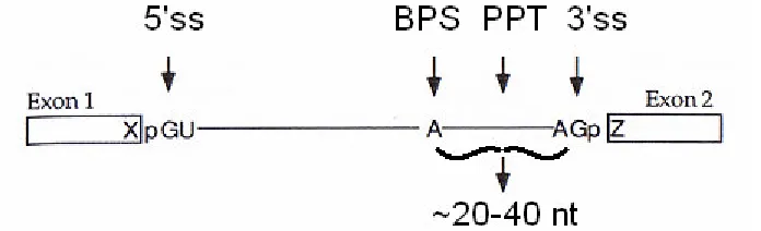
sequences coordinate with the spliceosome to perform the act of splicing: donor

splice site (5’ splice site), branch point sequence (BPS), polypyrimidine tract

(PPT), and acceptor splice site (3’ splice site) [6] (Figure 3).

Figure 3: The Signals of Splicing(adapted from: [5]). Four known intronic signals coordinate splicing: donor splice site (5’ss), branch point sequence (BPS), polypyrimidine tract (PPT), and acceptor splice site (3’ss). Reading an intron from 5’ to 3’, the signals occur in the aforementioned order. The donor splice site marks the border between the upstream exonic (Exon 1) and the downstream intronic regions. Conversely, the acceptor splice site marks the transition from the upstream intronic region to the downstream exonic region (Exon 2). In humans, the BPS and PPT usually, but not always, reside in close proximity to the acceptor splice site.

Splicing begins with the base pairing of the U1 snRNA of the spliceosome to the

donor splice site [5] consensus sequence MAGGURAGU (where M is an A or C

and R is an A or G) [6]. The next step involves the usage of the BPS which is

recognized by snRNA U2 [5]. The BPS has a consensus sequence of YYRAY

(where Y is a C or T) and in humans is normally located approximately 20-40

nucleotides upstream of the acceptor splice site [5], but it has been shown to

exist as far as 400 or more nucleotides upstream [7]. The adenosine within the

BPS reacts with the donor splice site in order to cleave the exon/intron border

leaving the 3’ end of the upstream exon free while the 5’ end of the intron joins

7

4). In the final step of splicing, the 3’ end of the recently cleaved upstream exon,

utilizing the PPT, acceptor splice site, spliceosome, and other splicing factors,

attacks the acceptor splice site (consensus sequence YAGR [6]) leaving the

newly spliced intron to be degraded while the two surrounding exons ligate [5,7].

Figure 4: Splicing Mechanism [5]. Splicing is carried out in three main steps.

Top: The spliceosome brings the donor splice site and the BPS together thus cleaving the Exon 1 - intron border and leaving the donor splice site attached to the BPS in a manner known as the lariat. Middle: The newly cleaved upstream exon (Exon 1) attacks the acceptor splice site thus cleaving the intron – exon 2 border. Bottom: The free ends of the exons are ligated together while the intron is left to be degraded.

The importance of splicing in eukaryotes cannot be overstated. Events that lead

8

half of disease-causing mutations [6] and are quite possibly the leading cause of

hereditary disorders [8]. Mutations in introns can cause exon skipping, usage of

aberrant 5’ and 3’ splice sites, and intron inclusions [8]. Such events can lead to

the addition or exclusion of peptides in the protein products or frame shifts which

can cause nonsense alterations in the mRNA sequence [7]. Some of these

improper transcripts may be able to escape RNA surveillance mechanisms [6]

while others are deleted due to nonsense mediated decay (NMD) [7]. Either way

this means that the incorrect transcript is produced which affects the expression

levels of the proper transcript.

Splicing is a significant event in any eukaryotic organism and although much

research has been devoted towards splicing, further work, especially in prediction

algorithms, is still warranted. The accurate prediction of splice sites would lead

to a better understanding of proper, alternative, and aberrant splicing. With

correct splice site prediction, scientists could acquire more information that could

lead to findings in gene expression, RNA regulation, and both proper and

aberrant protein structures. Although a reasonable amount of information is

known and available about splicing and the signals, proteins, and other factors

involved, the prediction of splice sites is still a difficult and often inaccurate

9

1.3 Problem Statement

3

The donor splice site is relatively easier to predict than the acceptor splice site

because it involves searching for a single nine nucleotide consensus sequence.

The acceptor splice site involves searching for a small, roughly four base

consensus sequence along with an approximately five nucleotide BPS

consensus and the PPT which may or may not be well defined. At times there

may be several potential BPS and/or acceptor splice sites. There may or may

not be total dominance by a candidate acceptor splice site. Competing splice

sites may be selected a certain percentage of the time, but may encounter RNA

surveillance mechanisms which eliminate the transcripts rendering them invisible

to in vivo experiments [7].

The prediction of acceptor splice sites is, indeed, a difficult task. There are

certain characteristics, however, that have recently been observed which may

offer some assistance. For example, the first AG dinucleotide downstream of the

BPS is usually part of the actual acceptor splice site [6,7]. Also, a search does in

fact take place in the absence of the authentic acceptor splice site and those

candidates that are more distantly located than others compete less efficiently

[6]. These findings have helped to shape a hypothesis that a scanning

mechanism is used to find the acceptor splice site [6,7]. The idea is that after the

spliceosome has located and dealt with the donor splice site, a search begins

from the BPS downstream until a suitable 3’ splice site consensus sequence is

10

Other acceptor splice site characteristics that may be useful in prediction

methods include PPT, AG dinucleotide exclusion zone (AGEZ), and nucleotide

dependency observations. Although the PPT is a complex and dynamic signal,

the probability of observing a splice site directly downstream increases when the

PPT is strong (full of C’s and T’s). A strong PPT is a good signal that a

candidate is indeed an actual splice site. The involvement of AG dinucleotides in

the acceptor splice site consensus sequences combined with the idea of a

scanning mechanism dictates that their presence prior to an acceptor splice site

would seemingly confound the splicing process. AGEZ refer to the observation

that AG dinucleotides are actually suppressed upstream of acceptor splice sites.

Also, nucleotides often depend on adjacent or nearby nucleotides. Discovering

and incorporating these dependencies into statistical methods can lead to

improved results.

The current state of splice site prediction tools consists of methods based on

nucleotide frequency matrices, machine learning approaches, neural networks,

information theory, Markov models, and maximum entropy models [8]. Of these

methods it has been noted that Markov models along with maximum entropy

models usually outperform the other techniques [5]. In comparison trials using

acceptor splice site data it was found that the first-order Markov model and the

maximum entropy model do indeed outperform the other methods with the

11

It has been the hope of this work that through exploration of splice site

characteristics, probabilistic approaches, and information models, findings that

aid in the prediction of acceptor splice sites will ensue. The following sections

include explanations about the data and information and subsequent results from

several statistical model approaches. Weight matrix, Markov, and log odds ratio

models have all been applied to the prediction of acceptor splice sites. The

results serve to verify the complex nature of this problem, but may also suggest

that the log odds ratio method is in fact a superior technique when compared to

12

2. Data

2.1 Construction

4

The data utilized was created by Burset and Guigo [9]. Their group began with

vertebrate sequences from GenBank release 85.0 (15 October 1994) and placed

a number of constraints upon it. The data were screened for a number of

characteristics resulting in what is widely considered a very ‘clean’ dataset.

The following factors were implemented in the cleaning of GenBank release 85.0

(Figure 5). All sequences that coded for partial proteins, had ambiguous splice

sites, complementary strand coding, pseudo genes, alternative splice sites, were

in excess of 50,000 nucleotides, or were submitted before 1993 (GenBank

release 74.0) were excluded. All sequences were then screened for proper start

and stop codons, correct reading frames, and proper splice site consensus

sequences.

The resulting data set included 569 sequences containing 2,077 introns and

2,646 exons. Beyond the Burset and Guigo restrictions, this work placed the

additional constraint of not allowing any redundant sequences into the data set.

An investigation of the data found 15 redundant sequences. After removal of the

redundancy, the data was comprised of 554 sequences with 2,040 introns and

13

Figure 5: Data Cleaning. The Burset and Guigo data set went through numerous cleaning stages. Included in this list are the steps Burset and Guigo took as well as an additional constraint placed on the data during this work. The final bullet, referring to the removal of redundant sequences, was an additional cleaning step not originally performed by Burset and Guigo.

The Burset and Guigo data set is especially useful in this work because of its

insistence upon accurate splice site consensus sequences. The accurate

prediction of splice sites is a difficult task. It is logical to conclude then that those

splice sites that present the most challenging prediction, presumably those with

improper consensus sequences, should be sought after when an algorithm that

can accurately predict well known and easily recognized splice sites is already in

place.

2.2 Observations

5

After obtaining the Burset and Guigo data set, the next task involved

characterizing the data. There are many ideas and methods one can employ in

making observations.

Nucleotide distributions are among the simplest observations of genomic data.

14

present an immediate challenge. Fortunately when classifying this work as a

problem in acceptor splice site prediction, a solution to varying sequence lengths

becomes clear. All intronic sequences were aligned utilizing their consensus

acceptor splice sites. Thus the observation of the nucleotide distribution within

the area directly upstream of an acceptor splice site becomes a more

straightforward task.

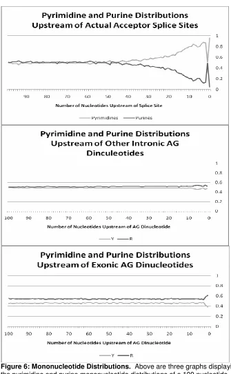
The consensus acceptor splice site sequence is an AG dinucleotide. Figure 6

allows for the comparison of the nucleotide distributions upstream of both splicing

and non-splicing AG dinucleotides. There is an obvious signal prior to those AG

dinucleotides that correspond to true acceptor splice sites while no signal exists

prior to other intronic and exonic AG dinucleotides. This is a vital observation as

this information is incorporated into the statistical models applied to splice site

15

Figure 6: Mononucleotide Distributions. Above are three graphs displaying the pyrimidine and purine mononucleotide distributions of a 100 nucleotide window upstream of AG dinucleotides. The consensus sequence for acceptor splice sites is an AG dinucleotide therefore an observation of the difference in signals prior to a splice site AG dinucleotide and a non-splice site AG

16

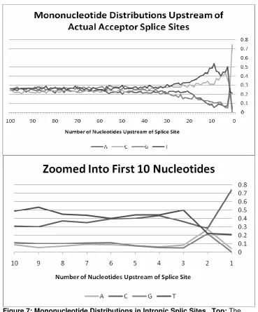
A look at all of the aligned sequences reveals a gradual signal prior to the splice

site often referred to as the polypyrimidine tract, or the PPT. Pyrimidines (C’s

and T’s) occur more frequently prior to a splice site than do purines (A’s and G’s).

The signal gradually increases in strength until just prior to the splice site where

there is a dip towards equal probabilities (Figure 7). The second position

upstream contrasts the rest of the signal. In an area where pyrimidines

predominate, this position observes equal frequencies of each nucleotide. The

first position upstream is skewed towards pyrimidines, particularly cytosines. In

fact, C’s are observed at high enough frequencies to where one can label the

acceptor splice site as having a consensus sequence of CAG.

As far as other intronic and exonic AG dinucleotides, no signals exist upstream.

A contrast of the regions upstream of splicing and non-splicing AG dinucleotides

is made in Figure 6. Those non-splicing AG dinucleotides residing within introns

contain pyrimidines and purines at roughly equal frequencies. Exonic AG

dinucleotides actually contain a small bias towards purines. This bias appears to

be fairly constant and although there is a small increase in purine frequency

upstream of AG dinucleotides in exonic regions, this is most likely due to codon

17

Figure 7: Mononucleotide Distributions in Intronic Splic Sites. Top: The overal gradual increase in frequency of both C and T coupled with the gradual decrease in frequency of A and G is easily observed. Two positions prior to the splice site all four nucleotides approach equal probabilities where their

frequencies are approximately 0.25, or 25%. The next position, however, shows a dramatic increase in C’s coupled with a decrease in A’s and G’s. Bottom: A close up of the first ten nucleotides upstream. A closer look more readily reveals the characteristics of the first and second positions.

Similar to these observations are those made by Lukas Habegger (Figure 8).

Habegger has performed a very similar analysis of a 400 nucleotide area

upstream of acceptor splice sites in the organism Leishmania major [10].

18

of splicing. The fact that the PPT signal exists in both lower eukaryotes like

Leishmania major and also in vertebrates is a testiment to the conserved nature

of the signal. However, unlike vertebrates, the Leishmania major signal is much

longer as it stretches for more than 200 nucleotides compared to the normal

20-40 in vertebrates. Another difference lies in the maximum strength of the signal.

The Leishmania major signal, while longer, obtains a maximum strength at

roughly 75% pyrimidine content while the vertebrate data reveals a signal that

reaches nearly 90% pyrimidine content.

Figure 8: Pyrimidine and Purine Distributions Prior to Leishmania major

19

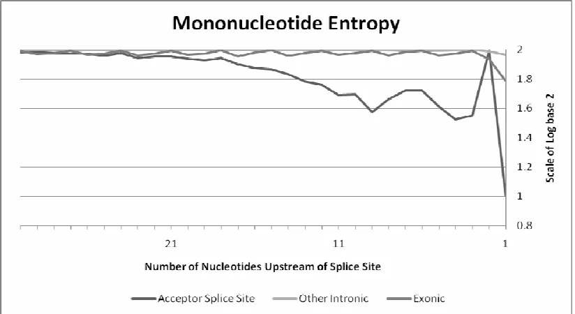
Because it is different in splice sites and non-splice sites, the polypyrimidine tract

becomes a valid means of discriminating between the two in the process of

splice site prediction. The amount of information obtained from utilizing this

signal can be viewed in the entropy graph contained in Figure 9. Entropy can be

described by the following formula:

2 1

( )

( ) log ( )

i

Entropy H X

p x

x

=

=

= −

Equation 1 [11]

where p(xi) can be the probability of a nucleotide or nucleotide combination (i.e.

p(A), p(C), … , p(T) or p(AA), p(AC), … , p(TT), etc…) and n is the number of

nucleotide combinations (i.e. n = 4 when considering mononucleotides [A,C,G,T]

20

Figure 9: Mononucleotide Entropy. Entropy, in this particular case, is the observation of how much information is gained through the examination of any given position prior to an AG dinucleotide. The more information a position holds, the closer to one its value will be. Those observations closer to two are very random while those observations closer to zero are nearing fixation, or are very non-random. There is a great deal more information within the positions prior to a splice site AG dinucleotide when compared to other, non-splice site AG dinucleotides.

Entropy can be seen as a measure of uncertainty. When something is

very random it is seen as uncertain. In a random situation where the

probabilities of mononucleotides are approximately equal, the entropy

would be close to two. In general, the maximum entropy value will be

log2(n). However, if something is not random at all, but we are instead

fairly certain of a position’s properties, the entropy would be close to zero

since as the p(xi) approaches one, the log2(xi) approaches zero. Figure 9

reveals that much more information is present in the signal prior to a splice

21

Another observation orignates from the idea that the spliceosome utilizes a

scanning mechanism in an attempt to locate a proper acceptor splice site. Recall

that once the spliceosome has found and dealt with the donor splice site, it scans

the sequence downstream of the branch point sequence (BPS) until an acceptor

splice site is found (Figure 4). It is logical therefore to suggest that there must be

a negative selection towards the presence of AG dinucleotides between the

branch point sequence and the actual acceptor splice site (Figure 10). The

resulting tracts devoid of AG dinucleotides are known as AG dinucleotide

exclusion zones, or AGEZ.

There does exist a depression in the frequency of AG dinucleotides observed

upstream of acceptor splice sites. There are exceptions, however, as the

frequency does not actually reach zero. There has been some speculation that

extra-intronic signals control the usage of candidate AG dinucleotides within

about a 12 nucleotide window upstream of the consensus splice site [3,4]. Work

to uncover these signals and how they work to achieve such a result is currently

underway [12]. If such extra-intronic signals exist, they would present a

confounding factor to this analysis. Since this work is focusing only on intronic

signals, it may be the case that AG dinucleotides within this 12 base pair window

upstream of the actual acceptor splice site are predicted to be actual splice sites

22

23

Another observation about the declining frequency in AG dinucleotides prior to a

splice site is that the signal is gradual. This implies that the AG exclusion zone is

not constant for every splice site. Again, current literature attempts to explain

such an observation [6,8]. The spliceosome machinery comes into contact with

the intron at the branch point sequence and covers an area of roughly 30

nucleotides (approximately 15 nucleotides on either side of the branch point

sequence). Because these nucleotides are essentially blocked from

consideration as a splice site by the splicing machinery, no negative selection

toward AG dinucleotides would exist allowing them to appear more randomly as

one moves towards the branch point and then beyond. Upstream of the branch

point AG dinucleotide appearance most likely becomes quite random. Adding to

the complexity of the signal is the fact that positioning of the branch point

sequence is inconsistant between the various sequences within the data. The

branch point sequence is usually 20 to 40 nucleotides upstream of the acceptor

splice site, but can be as far as roughly 400 nucleotides upstream [7]. When this

information is averaged together over an entire data set, the result is a slow,

gradual signal.

The idea of comparing distances between AG dinucleotides to identify splice

sites is an appealing one, but becomes difficult because of the short branch point

sequence-acceptor splice site distance observed in vertebrate genomes. Also,

the comparison of other dinucleotide exclusion zones to these AG exclusion

24

negative selection of AG dinucleotides prior to both splice and non-splice sites.

In each graph there is a line representing how often the AG dinucleotide should

occur at random compared to how often it was observed. There is a distinct

decrease in the observation of AG dinucleotides prior to the splice site. The

non-splice site AG dinucleotides actually exhibit a higher frequency of AG

dinucleotides than what would have been expected at random.

Figure 11: CG Dinucleotide Distribution. Prior to the acceptor splice site, the CG dinucleotide is also found less than would normally be expected. This is not, however, a characteristic of a splice site, but rather a characteristic of CG dinucleotides across many genomes. The CG dinucleotide is actually

25

2.3 Goal

1

With a good idea of what is going on in the nucleotides prior to acceptor splice

sites it is now appropriate to attempt to create models which can accurately

predict said splice sites. The goal of this work is to increase the accuracy of

acceptor splice site prediction. One key assumption is that donor splice site

prediction has already been completed. This work assumes that, either through

an accurate prediction method or through experimental work, the donor splice

sites have been accurately identified. This leaves the other half of the splice site

prediction problem yet unsolved. Prediction of both donor and acceptor splice

sites resides within the realm of gene finding. Breaking the vastly complicated

issue of gene finding into smaller parts is a logical and less confusing

methodology that may yield different approaches for prediction of the various

gene signals. This work utilizes three models: a weight matrix model (WMM), a

Markov model, and a log odds ratio model and discusses the use of a fourth,

non-probabilistic model. While the log odds ratio model has proven to be the

best of the three, there is certainly room for improvement in this most challenging

26

3. Weight Matrix Models (WMMs)

3.1 Overview

6

Probabilistic models provide a very intuitive and accepted approach to analyze or

predict genomic sequence characteristics. When based on genomic sequences,

probabilistic models assign probabilities to nucleotide occurrences, or

combinations, over specified regions. Nucleotide occurrences refer to whether

mono-, di-, tri-, etc. nucleotides are being observed. Variability in probabilistic

models occurs when one considers how to obtain probabilities, where and how

often to assign probabilities, and over what genomic distance the model should

operate.

Weight matrix models form a subset within probabilistic models [5,13]. A window

of nucleotides is often observed but there are varying approaches as to how the

window is analyzed. The first, a simple approach referred to here as a ‘block’

method, would be to use a single nucleotide probability matrix across the entire

window. A second method, referred to here as the positional approach, would be

to assign a nucleotide probability matrix for each position within a window of

nucleotides.

The block approach to weight matrix models involves assigning probabilities to

nucleotide occurrences over a specified window (Figure 12A). In other words,

27

window as it is at the end of the window thus the probabilities are independent of

position. A general formula for this approach is given by

1 2

1

( )

( ) ( )... ( )

( )

i

p X

p x p x

p x

p x

=

=

=

∏

Equation 2 [5]

where xi is a nucleotide combination, p(xi) is the probability of said nucleotide

combination, and is the length of the window being observed.

A good example of how a block approach works can be explained through a die.

If one is looking at mononucleotide probabilities, a four-sided die becomes

appropriate. The die will be weighted to reflect the probabilities of the four

nucleotides. When the die is rolled times, the resulting sequence should

contain a proportion of nucleotides that correctly reflects the probabilities

observed in a training data set. In other words, this means that the resulting

sequence will have the correct nucleotides, but will not be able to place those

nucleotides in the correct position or order. The positional approach, as its name

28

The position specific approach involves assigning probabilities to nucleotide

occurrences based on their position within a specified window (Figure 12B). In

other words, the probability of one nucleotide occurrence can be different at the

beginning of the window than the probability of the same nucleotide occurrence

at the end of the window. A general formula for the positional approach is given

by

A) B)

…A C C G T T C C … …T T G C A A T T … …C G A A T G A C …

p(A) p(C)

p(G) p(T) p(A) p(C)

p(G) p(T) p(A) p(C)

p(G) p(T) p(A) p(C)

p(G) p(T) …ACCGTTCCCACC… …TTGCAATTAGAT… …CGAATGACATGA…

29

(1) (2) ( ) ( )

1 2

1

( )

( )

( )...

( )

( )

i i

p X

p

x p

x

p

x

p

x

=

=

=

∏

Equation 3 [5]

where xi is a nucleotide combination, p(i)(xi) is the probability of said nucleotide

combination in position i, and is once again the length of the window being

observed.

Following the loaded die example, imagine now that there are dice available,

where is equal to the length of the window being observed. Each die is

weighted specifically to its positional probabilities. This means that die1 can have

a different probability distribution than die . When the dice are rolled, die1 is first

considered followed by die2 through die . The result is a sequence that should

30

3.2 Results

7

Both the block and positional approaches were run using 10-fold cross validation.

There were 2,040 intronic sequences, of which 90%, or 1,836, sequences were

selected to train the model while the remaining 204 sequences (10%) were

utilized in the test set. This process was then repeated 10 times.

… A C G A T T …

p(A) p(C) p(G) p(T)

P(3)_(A)

p(3)_(C)

P(3)_(G)

p(3)_(T)

P(2)_(A)

p(2)_(C)

P(2)_(G)

p(2)_(T)

P(1)_(A)

p(1)_(C)

P(1)_(G)

p(1)_(T)

p(A)p(C)p(G)…

p(1)(A)p(2)(C)p(3)(G)…

Figure 13: Testing a Weight Matrix Model. The graphic above displays the testing methods for the block and positional weight matrix models (A & B respectively). A. The block method utilizes a single probability matrix over an entire window. The observed probabilities are then

31

There are two variables associated with a weight matrix model. Both window

size and nucleotide combination can be altered between WMM applications.

Figure 7 reveals a signal prior to the splice site. Therefore window size becomes

an important variable in capturing this signal. Secondly, nucleotide combinations

should be taken into account. A model may incorporate mononucleotides,

dinucleotides, etc… This WMM utilized mononucleotides, dinucleotides, and

trinucleotides over a range of window sizes varying from 15 to 50 nucleotides in

increments of 5 (Figure 14 and Figure 15).

Over all variables, the positional approach consistently outperformed the block

approach. When observing mononucleotides with an increasing window size, the

positional approach obtained a fairly constant positive predictive value and

accuracy while the block approach gradually decreased in both measures. The

same observations can be generalized to the dinucleotide and trinucleotide

combinations. Within the positional models, both the positive predictive value

and the accuracy increase as one progresses through the nucleotide

combinations. The trinucleotide variable resulted in the best accuracy and

positive predictive values.

Accuracy is calculated by averaging the sensitivity and selectivity. Sensitivity

32

TruePositives

Sensitivity

TruePositives FalseNegatives

=

+

Equation 4

TrueNegatives

Selectivity

TrueNegatives FalsePositives

=

+

Equation 5

It then follows that accuracy is:

2

Sensitivity Selectivity

Accuracy

=

+

Equation 6

The positive predictive value is a statistic that can be used to describe a situation

in which there are many more negative results than positive results. That is,

there are many candidate AG dinucleotides that are not true splice sites while

there are relatively few true acceptor splice site AG dinucleotides. The large

number of non-splicing candidates provides for noisy results that can best be

described by the positive predictive value statistic. The positive predictive values

can be calculated by equation 7:

TruePositives

PPV

TruePositives FalsePositives

=

+

33

Figure 14: Positive Predictive Value (PPV) VS. Window Size. The positional approach performs much better than the block approach in all WMM applications.

Top: The PPV when a mononucleotide WMM is applied. The positional

34

Figure 14 shows that the positive predictive value continues to increase as the

window size increases. There are many false positives associated with acceptor

splice site prediction. As the window size increases, there is a slight gain in

selectivity which, through the reduction of false positives, raises the positive

predictive value. However, even though there is a slight increase in selectivity,

there is an accompanied decrease in sensitivity. The decrease in sensitivity is

enough to offset the gains in selectivity as the accuracy (an indicator of both

sensitivity and selectivity) also begins to decline. The peak accuracy occurs at a

window size of 35 nucleotides with trinucleotide observations. These will be the

variables by which weight matrix models are compared to the other probabilistic

models. A summary of the results from the weight matrix model given a window

size of 35 nucleotides and trinucleotide observations can be viewed in Table 1.

The previous statements have hit upon the importance of the positive predictive

value. With such a large number of potential false positives, a statistic that

reveals how confident one can be that predicted splice sites are actual splice

sites becomes necessary. Because of the importance of the positive predictive

value, it may be necessary to consider it to be more important than other more

widely used statistics such as accuracy. Small increases in selectivity will

exclude a large number of false positives while a small increase in sensitivity will

include a small number of additional true positives. In this light, accuracy does

not track well with this situation. The positive predictive value, on the other hand,

35

36

Table 1: Summary Statistics for positional WMM at Window = 35 and Using Trinucleotide Observations. The weight matrix model obtains fairly high sensitivity, selectivity, and accuracy statistics. However, the positive predictive value leaves much to be desired.

Averages TP FP TN FN Sensitivity Selectivity PPV Accuracy

- 188.2 829.8 8972.3 15.8 92.25 91.56 18.72 91.91

The block approach also observed its best results utilizing trinucleotide

observations. The best window size, however, was observed to be 15

nucleotides. When the window size increased, the block weight matrix model’s

performance decreased dramatically. The optimal conditions are displayed in

Table 2.

Table 2: Summary Statistics for block WMM at Window = 15 and Using Trinucleotide Observations. The weight matrix model obtains a good deal of sensitivity, but has a relatively low selectivity. In the problem of acceptor splice site prediction, selectivity greatly alters the positive predictive value, as can be seen in these results.

Averages TP FP TN FN Sensitivity Selectivity PPV Accuracy

- 189.2 1451.2 8350.9 14.8 92.75 85.25 11.71 89.00

There is biological relevance as to why the optimal window size differs between

the block and positional approaches. The signal prior to an acceptor splice site is

very strong within the first 15 to 20 nucleotides, but tapers off gradually as one

moves farther away (Figure 7). The block approach will then convey that strong

signal in a small window size, but as the window size increases, the signal is

dampened as the strong region of the signal is averaged in with weaker regions.

The positional approach, however, is not negatively affected by the same window

37

signal and the weaker signals farther upstream without immediately averaging

them together. This essentially allows the positional approach to use the same

strong signal that a block approach has in a window size of 15 and then to apply

further signal information farther upstream to try and decipher splicing vs.

non-splicing to a more accurate extent.

Although simple to understand and easy to implement, weight matrix models are

still lacking on some fronts. Most noticeably, weight matrix models do not

incorporate the idea of dependency. Weight matrix models are allowed to

multiply probabilities along a given sequence because of the assumption of

independence between the nucleotides. Independence, however, is most likely

not the case for any given nucleotide sequence. The prerogative then exists to

utilize a model that incorporates dependencies. A good example of such an

approach lies within another subset of probabilistic models known as Markov

38

4. Markov Models

4.1 Overview

8

Like weight matrix models, Markov models are a subset of probabilistic models.

[5,13] Discriminating between the two models is the idea of dependency. Often,

the nucleotides of a genomic sequence will maintain relationships with either

adjacent or nearby nucleotides. Such relationships have ramifications on the

types of statistical models used to predict them. No longer can a model assume

independence without incorporating the correct dependency.

Markov models allow for dependencies to exist. A homogeneous Markov model

that observes dependencies among adjacent nucleotides can generally be

described as: 1 1

(

,

)

(

|

)

(

)

ij t t

t

P X

j X

i

p

P X

j X

i

P X

i

+

+

=

=

=

=

= =

=

Equation 8 [14]

where pij is the probability of observing j in position t+1 given i in position t. X is

the nucleotide sequence with i and j being from the state space S={A,C,G,T}.

The above model thus incorporates the dependency between the nucleotide

39

The formula given above is considered a 1st _{order Markov model because it}

incorporates one order of dependency. Given enough data, Markov models can

be extended to higher orders. The equation for a 2nd _{order homogeneous}

Markov model looks like:

2 1 2 1 1

(

,

,

)

( )

(

|

,

)

(

,

)

t t t

ijk t t t

t t

P X

k X

j X

i

p t

P X

k X

j X

i

P X

j X

i

+ + + + +

=

=

=

=

=

=

= =

=

=

Equation 9 [14]

where pijk is the probability of observing k in position t+2 given j in position t+1

and i in position t. X is once again the nucleotide sequence with i, j, and k being

from the state space S={A,C,G,T}. This Markov model now incorporates

nucleotide dependencies from the previous two observations upstream.

Markov models can be trained in much the same manner as described in the

weight matrix model chapter. However, the observation of dependencies, as

described in the formulas above, needs to be incorporated in both the training

and testing models.

Once again, the model can be broken into block and positional approaches.

When probability transition matrices have been formed in a manner very similar

to Figure 12, they are used in order to score the remaining sequences (Figure

40 p(A|A) p(A|C) p(A|G) p(A|T) p(C|A) p(C|C) … p(T|G) p(T|T) p(C|A)p(G|C)p(A|G)p(T|A)

A C G A T _… A C G A T

p(A|A) p(A|C) p(A|G) p(A|T) p(C|A) p(C|C) … p(T|G) p(T|T) p(A|A) p(A|C) p(A|G) p(A|T) p(C|A) p(C|C) … p(T|G) p(T|T) p(A|A) p(A|C) p(A|G) p(A|T) p(C|A) p(C|C) … p(T|G) p(T|T) …

p(C|A) = p(A,C)/p(A)

p(C2|A1) = p(A1,C2)/p(A1)

p(G|C) = p(C,G)/p(C) p(T|A) = p(A,T)/p(A)

p(G3|C2) = p(C2,G3)/p(C2) p(T5|A4) = p(A4,T5)/p(A4)

p(C2|A1)p(G3|C2)p(A4|G3)p(T5|A4)

A C G A T

Figure 16: Scoring of a Markov Model. The above diagram indicates the method by which sequences are scored using both a block and positional 1st order Markov model. A:

41

4.2 Results

9

In congruence with the weight matrix model, both the block and positional

approaches were run using 10-fold cross validation. Once again, a variety of

variables exist within Markov models. The same window sizes used in testing

the weight matrix models were also used in testing the Markov models.

Nucleotide combinations, however, were different between the two models.

Where weight matrix models use mono-, di-, and tri- nucleotide combinations, the

Markov models utilize 1st order, 2nd order, 3rd order, etc… These particular

models were run with both 1st _{and 2}nd _{order using both block and positional}

approaches (Figure 17 and Figure 18).

As was the case with the WMM results, the block approach decreased in both

positive predictive value and accuracy as the window size increased. The

positional approach obtained relatively better results than the block approach.

The best results, however, are observed over two different parameters. The

highest positive predictive value is obtained by the positional 2nd order Markov

while the best accuracy is achieved by the 1st _{order Markov. As the window size}

increases, the 2nd order Markov model observes a gradual increase in positive

predictive value while the 1st _{order Markov remains fairly constant. The accuracy}

obtained over the two parameters remains roughly constant over window size

with the 1st order Markov achieving greater accuracy over the 2nd order Markov in

all window sizes. The results of the optimal conditions for both models can be

42

Figure 17: Positive Predictive Value VS. Window Size. The Markov models show somewhat similar results to the weight matrix model. The positional Markov model consistantly outperforms the block model. Top: The 1st order Markov models. The positionally trained Markov model outperforms the block model. The block model’s PPV decreases with window size while the position increases. Bottom: The 2nd _{order Markov models. Once again the positionally}

43

Figure 18: Accuracy VS. Window Size. Once again, the Markov models show somewhat similar results to the weight matrix model and the positional Markov model consistantly outperforms the block model. Top: The 1st order Markov models. The positionally trained Markov model outperforms the block model. The block model’s accuracy decreases with window size while the position increases. Bottom: The 2nd order Markov models. Once again the positionally trained Markov model outperforms the block approach. The block approach’s accuracy declines with window size while the positional approach increases. Overall, 1st order Markov obtains the highest accuracy.

Table 3: Summary Statistics for 1st and 2nd Order Positional Markov Models at Window = 25 and 50 Respectively. The 1st _{order Markov model achieved}

the highest accuracy at a window = 25. However, the 2nd order Markov achieved the highest positive predictive value at window = 50.

Averages TP FP TN FN Sensitivity Selectivity PPV Accuracy

1st Order 194.5 927.8 8321.6 9.5 95.34 89.96 17.4 92.65

44

Figure 17 and Figure 18 reveal the superiority of the positional approach over the

block approach. Once again this has to do with the gradually increasing intensity

of the signal as it approaches the acceptor splice site. The exact reasoning can

be explained in an assumption of Markov models known as homogeneity.

Homogeneity refers to the fact that a Markov model expects its transition matrix

to be independent of time, as shown in the following formula:

1 1

(

|

)

(

|

)

P X

=

j X

= =

i

P X

=

j X

=

i

Equation 10

where the probability of going from nucleotide i to nucleotide j is the same for all

s and t in sequence X. The block approach will clearly violate this assumption.

For example, the probability of observing an AG dinucleotide (G given an A)

differs greatly 100 base pairs upstream from an acceptor splice site when

compared to 10 base pairs upstream (Figure 19). The positional approach offers

a method of bypassing the homogeneity assumption as a transition matrix only

45

Figure 19: Probability of a G Given an A. The probability of observing a G given an A decreases dramatically as one approaches an acceptor splice site. Homogeneity does not hold for this sequence as the probability of a G given an A is different at different times, or positions within the sequence.

Because there is ambiguity with regard to which Markov model is best, both of

them are compared to the best weight matrix model result (positional,

trinucleotide WMM) (Figure 20). The weight matrix model splits the two Markov

models in both positive predictive value and accuracy. Where the 2nd _order

Markov model is superior in positive predictive values, the weight matrix model

performs better than the 1st _{order Markov model. Conversely, where the 1}st _order

Markov model is superior in accuracy, the weight matrix model performs better

46

Figure 20: Markov Model Compared to Weight Matrix Model. The positional Markov models compared to the best weight matrix model, the positional trinucleotide approach. Top: The 2nd order Markov model obtains a higher positive predictive value than both the 1st _{order Markov and the weight matrix}

model, althogh the weight matrix model does achieve a higher PPV than the 1st

order Markov. Bottom: The 1st order Markov achieves the highest accuracy followed by the weight matrix model and then the 2nd order Markov.

Markov models offer slightly different results than the weight matrix model,

but there are no large gains in accuracy or positive predictive value. A

Markov model may meet limitations when considering the assumption of

homogeneity. This can be side stepped by utilizing the positional

47

describe higher orders of dependency by the size of the data set. When

one attempts to observe higher orders of dependency, certain

observations will become very rare. Such observations do not occur often

enough to create an informative model. A method of circumventing this

concern has been described by Burge [5] and is called the Maximal

Dependence Decomposition, or MDD.

4.3 Maximal Dependence Decomposition (MDD)

10

Often, there is insufficient data when attempting to perform higher order Markov

models. Burge explains an alternative method of exploring higher orders of

dependency. Through the use of an MDD, it is possible to observe which

positions contain the most dependency in a group of sequences [5].

The general idea of an MDD is to create a matrix of chi-squared scores. The

formula for a chi-squared test is as follows:

2

, ,

2

, _,

(

)

i j _{i j}

O

E

X

E

−

=

Equation 11 [15]

where X2is the chi squared value, Oi,jare the observed values, Ei,j are the

expected values, and i and j are from the set S={A,C,G,T}. The expected values

48

.

.

O O

E

N

×

=

Equation 12 [15]

where Eijis the expected value and Oi. and O.jare the observed values. N

represents the total number of observations. Each X2 can therefore be broken

down into a matrix of its observed values:

AA AC AG AT

CA CC CG CT

GA GC GG GT

TA TC TG TT

O

O

O O

O

O

O O

O

O

O O

O

O

O

O

Equation 13 [15]

where the Oij’s are the observed values and N is the total number of observed

values. O.Arepresents the number of A’s within position i and OA. represents the

number of A’s within position j.

Each position within a window of nucleotides is compared to every other position

such that a chi-squared matrix is formulated.

Position i

A C G T P

o A s i C t i G o n T

j

O

.

O

.

O

.

O

.

49

2 2

1,2 1,

2 2,1

2 ,1

0

0

n

n

X

X

X

X

Equation 14 [15]

Within the chi square matrix, the diagonal consists of zeros as positions

compared to themselves that will not aid the MDD in determining maximal

inter-positional dependencies. The matrix is also symmetrical about the diagonal as

the chi-squaredof i,j is equal to the chi-squared of j,i.

In summary, the nucleotide composition of each position is compared to one

another and a matrix is formulated as seen in Equation 13. From said matrix, a

X2 value can be computed via Equation 11. These X2 values are then placed into

a chi squared matrix as per Equation 14. The sum of the values in row 1 from

the chi squared matrix will yield a value describing the importance of position 1.

The sum of the values in row 2 will describe the importance of position 2 and so

on. The higher the sum, the more important the position where the highest sum

describes the position with the most ‘pull’ or dependency in the sequence.

A graph depicting these row sums thus describing the importance of positions

upstream of the splice site can be viewed in Figure 21. Figure 21 reveals the

interdependence between the first 100 nucleotides upstream of the acceptor

50

positions of importance have been declared, it is possible to split the data set on

these positions. In other words, when a position of interest has been found, for

example position = 4, the data set can be split into four data sets: position 4 = A,

position 4 = C, position 4 = G, and position 4 = T. Then the entire chi square

table is recalculated for each data set such that the next position of importance

can be found. For example, if split on position = 4 where position 4 = A, then the

next position of importance is position 61.

Figure 21: Resulting Chi Square Values From the MDD. There are three points that are very close to the same level of significance: 4, 27, and 63. These are the points that reach a chi squared score of approximately 3,000.

Table 4: MDD Results. The MDD revealed three positions of interest. Listed is the score of each of the poisitions that were used to split the data upon.

Position 4 27 63

Score 2986.56 2979.73 3003.19

The splitting of the data set allows the MDD to show more than one layer of

51

require enormous amounts of data in order to test for higher orders of

dependency. With MDDs one can split the data on an important position, find the

next most important position, and then split the data again. This process can be

carried out as long as there is sufficient data. The positions of importance then

reveal where higher order dependencies may exist.

Table 5: MDD Split Upon Position 4. The following tabe is an example of how the resulting data when the MDD splits upon a position of importance.

Nucleotide A C G T

Number of

Sequences 131 892 111 905

Next Position of

Importance 61 44 61 3

Table 5 depicts the results obtained when splitting an MDD upon a position of

importance, in this case position four. There are 131 sequences with an A in

position four and, when the MDD is run using only these 131 sequences, the next

position of maximum dependency is 61. Interestingly, an MDD analysis on the

111 sequences with a G in position four also found that position 61 was the next

maximum dependency position. When setting position four equal to a C, 892

sequences are included in the MDD and 44 becomes the next maximum

dependency position. Finally, when position four is a T, 905 sequences are

included in the MDD and position 3 is considered the next maximum dependency

position. A similar analysis was performed on positions 27 and 63 and can be

52

A very interesting observation that can be drawn from the MDD results involves

the comparison with Lukas Habeggar’s MDD on Leishmania major. Mr.

Habeggar saw similar results in that he split on position 26 in his work. Since

position 27 held a high level of significance in this vertebrate data set, the fact

that Habeggar observed position 26 as being very important in Leishmania major

suggests a conserved nature around these two positions. When considering the

biology of splice sites, these two positions may reflect the location of the branch

point sequence (BPS) within the splicing machinery. Currently, the BPS is an

extremely difficult signal to locate and has vexed those who have attempted its

prediction. The observation of maximum dependency at this position may reflect

the location of the BPS thereby making these results of great interest. Also, a

recent work from Lücke et al [] highlights differences between lower and higher

eukaryotic branch point sequences. Lower eukaryotes are though to have

relatively well defined branch point sequences when compared to higher

eukaryotes which observe more ambiguous branch point sequence signals.

These findings are reinforced by the MDD comparison between Leishmania

major and vertebrates. Lukas Habegger’s MDD results reveal a well defined

position of maximum dependency while this work’s vertebrate investigation

53

5. Log Odds Ratio

5.1 Overview

11

Probabilistic models represent an intuitive and accepted approach in the

modeling of genomic signals. The comparison of two probability models (i.e. two

Markov models or two WMM models) is a conventional meth