Single-Determinant Theory of Electronic Excited States and Many-Electron Integrals for Explicitly Correlated

(1)

Single-Determinant Theory of Electronic

Excited States and Many-Electron

Integrals for Explicitly Correlated

Methods

Giuseppe Maria Junior Barca

June 2017

A thesis submitted for the degree of Doctor of Philosophy

of the Australian National University

c Copyright by Giuseppe Maria Junior Barca 2017

(2)

(3)

Declaration

The work described in this thesis, to the best of my knowledge, is original and does

not contain material that has been submitted for a degree or diploma at any other

University or College.

Giuseppe M. J. Barca

(4)

(5)

Acknowledgements

Now let me dispel a couple of rumors so they won’t fester into facts ... Yes! Before

beginning this doctorate I had a passion for mathematics and quantum mechanics. And

no, at the time when my supervisor, Prof. Peter Gill, first met me, I was not the man of

science you see before you. He found me in a dying country, where only the lovely bones

of an ancient intellectuality remain. “I was the intellectual equivalent of a 98-pound

weakling. I’d go to the beach and people would kick copies of Byron in my face.”

This doctoral candidacy has represented the opportunity of my life and I am indebted

with my deepest gratitude to my supervisor. Peter believed in me when my own people

did not. During this three years and a half, not only he has been an one-o↵scientific

mentor, but also and especially a friend and a father to me. His combination of scientific

acumen and unshakeable patience provided a fertile ground where my creativity and

analytic skills thrived reaching unprecedented levels.

My heartfelt thanks go also to Dr. Andrew Gilbert. His outstanding technical and

theoretical aid and his extreme thoughtfulness were crucial factors for the successful

fulfilment of my doctorate. I will always retain in my heart countless hours of scientific

discussions that he endured with great lenience. I will never forget his precious friendship,

but this is another story.

I am extremely grateful to my friend Dr. Pierre-Francois Loos (Titou). His very

hard-working attitude and enthralling enthusiasm for the field engaged me in many exciting

and productive ‘theoretical’ adventures. Without Titou’s support and collaboration a

good part of the research work included in this thesis would have not been possible at

all.

Thanks to the past and present members of the Gill group whom I have had the

(6)

particular Dr. Caleb Ball, who has been a very enjoyable and benevolent companion

for more than three years now, and Simon McKenzie, who, inter alia, together with Dr.

Ball, had the bravery of proofreading this thesis.

Special thanks to Prof. Jacob Katriel for providing me with many very useful

comments on this thesis.

I am also grateful for the generous financial support I received for the duration of

my doctoral studies in Canberra, and, in particular, the University Research Scholarship

from the Australian National University.

I wish also to thank Dr. Jia Deng for his unselfish friendship and his extraordinary

private support.

Furthermore, I wish to thank the entire Gill family for welcoming me as one of them.

I am greatly thankful to my wife for morally sustaining me in this and many other

hard choices, and for tolerating me during these years. Thank you for your courage and

your love.

I thank my parents who supported with great patience my pursuit of manifold

interests and encouraged me to endure when all seemed unsurmountable.

Last but not least, I thank my grandfather. He inspired me throughout my life,

instilling the seeds of perseverance, courage and dignity. I owe to him who I am today.

Giuseppe M. J. Barca

(7)

(8)

nobody has yet thought concerning that which everybody sees.”

(9)

Abstract

The aim of this thesis is twofold.

Its first part, Part A, is concerned with the development and assessment of a

single-determinant theory for electronic excited states. The theory is based on two simple

algorithms for finding excited-state solutions to self-consistent field (SCF) equations,

the Maximum Overlap Method (MOM) and the Initial Maximum Overlap Method

(IMOM). The extent to which these higher SCF solutions are useful approximations

to excited states is examined in diverse case studies, including challenging instances

such as double excitations, conical intersections and charge-transfer states. Results

indicate that single-determinant models yield, in most cases, accurate approximations to

electronic excited states, even for difficult excitations where other low-cost excited-state

methods either perform poorly or fail completely.

In Part B, we present efficient methods for the accurate evaluation of many-electron

integrals arising in the explicitly correlated electronic structure theory. In our

com-putational schemes efficient screening techniques, which adopt newly developed upper

bounds, are used to sift out the tiny fraction of integrals which are significant. Then,

non-negligible integrals are evaluated via recurrence relations that represent the

general-ization to three and four-electron integrals of two-electron integrals contraction-efficient

schemes such as the Head-Gordon-Pople and PRISM algorithms. In this way, we

devel-oped general computational schemes for integrals arising from the use of a wide class

of multiplicative correlation factors of the form f12 = f(|r1 r2|) and more specific

methods for many electron integrals involving Gaussian Geminals. Our results support

the evidence that our Gaussian-Geminal-based schemes yield a dramatic reduction of

(10)

(11)

List of Publications

The following manuscripts have been published as a direct consequence of the work

undertaken for this thesis:

Chapter 3 : G. M. J. Barca, A. T. B. Gilbert, and P. M. W. Gill

“Hartree-Fock description of excited states of H2”,

J. Chem. Phys. (Communication) 141, 111104 (2014).

Chapter 4 : G. M. J. Barca, A. T. B. Gilbert, and P. M. W. Gill “Simple models for difficult electronic excitations”,

J. Chem. Theory Comput.,submitted.

Chapter 5 : G. M. J. Barca, A. T. B. Gilbert, and P. M. W. Gill

“The excitation number: A tale of misassigned multiply excited states”,

J. Chem. Theory Comput. (Letter),submitted.

Chapter 7 : G. M. J. Barca, P.-F. Loos, and P. M. W. Gill

“Many-electron integrals over Gaussian basis functions. II. Upper bounds”,

J. Chem. Theory Comput.,in preparation.

Chapter 8 : G. M. J. Barca, P.-F. Loos, and P. M. W. Gill

“Many-electron integrals over Gaussian basis functions. I. Recurrence relations for

three-electron integrals”,

J. Chem. Theory Comput. 12, 1735 (2016).

Chapter 9 : G. M. J. Barca, and P.-F. Loos

“Recurrence relations for four-electron integrals over Gaussian basis functions”,

Adv. Quantum Chem., in press (2017), available online: https://doi.org/10.

(12)

Chapter 10 : G. M. J. Barca, and P. M. W. Gill “Two-electron integrals over Gaussian geminals”,

J. Chem. Theory Comput. 12, 4915 (2016).

Chapter 11 : G. M. J. Barca, and P.-F. Loos

“Three- and four-electron integrals involving Gaussian Geminals: fundamental

integrals, upper bounds and recurrence relations”,

(13)

Fundamentals of Quantum

[image:21.595.146.491.395.718.2]

Chemistry

(22)

1.1 From Schr¨

odinger to Quantum Chemistry

In principle, the electronic structure and the properties of any molecule in whichever

of its quantized states can be determined by solving the Schr¨odinger equation. The

equation reads

ı_~@

@t =H (1.1)

where_His the Hamiltonian for the system, _~is Planck’s constant divided by 2⇡ and ı

is the imaginary unit. The elusive entity denoted by is the so-called wave function,

a function of the spatial and spin coordinates of the particles (and of time), and it

encloses all the information about the system. The latter fact is also known as the first

postulate of quantum mechanics.

It is certainly one of the eccentricities of quantum mechanics that even if the state

of a system is completely specified by , the wave function itself does not have any

physical interpretation. However, the accepted view, which goes back to Born, is that

the square of the absolute value of wave function | |2 _{represents a probability density}

distribution.

At first glance Eq. (1.1) might seem innocuous to the reader, however much

complexity is hidden in the Hamiltonian term. For isolated molecules, ignoring relativity

and electromagnetism, the Hamiltonian takes the form

H⌘H(r,R)

=

N

X

i

~2

2mer

2

i M

X

A

~2

2MAr

2

A N

X

i M

X

A

ZAe2

|ri RA|

+

N

X

i<j

e2

|ri rj|

+

M

X

A<B

ZAZBe2

|RA RB|

(1.2)

wherer2

i is the Laplacian operator,

r2i =

@2

@x2

i

+ @

2

@y2

i

+ @

2

@z2

i

, (1.3)

M is the number of atomic nuclei,N is the number of electrons in the system,RAis the

(23)

me andeare the electronic mass and charge as well asMAandZA are the nuclear mass

and charge of theA-th nucleus.

The notation _H(r,R) in Eq. (1.2) is to explicitly highlight the dependence of the

Hamiltonian operator on the entire set of electronic and nuclear coordinates r⌘{ri}

andR_⌘_{RA}. It also suggests a significant fact: the Hamiltonian is time-independent.

This implies that Eq. (1.1) is separable in time and space-spin parts, i.e. its solution

can be written as the product

(x,R, t) = (x,R)⇥(t) (1.4)

of a purely spatial-spin part (x,R) and a purely temporal term⇥(t), where x_⌘_{xi}

is a shorthand notation to compactly represent the dependence on all the variables

xi⌘{ri, si}, withsi being the spin of the i-th electron.

Using the ansatz of Eq. (1.4) for the wave function and solving the di↵erential

equation for ⇥(t) yields

⇥(t) = exp

✓

ıEt

~ ◆

(1.5)

which leaves us with the time-independent wave equation[1, 2]

H(r,R) (x,R) =E (x,R) (1.6)

Equation (1.6) is an eigenvalue equation. For any physically meaningful system the

H(r,R) operator is Hermitian, and in order for Eq. (1.6) to yield physically acceptable

solutions, the wave function (x,R) must satisfy the following normalization condition

Z

| (x,R)|2dxdR= 1 (1.7)

which ultimately stems from the probabilistic interpretation. Since the integral must be

finite, the wave function is also required to comply with a square integrability boundary

condition. Solving the equation is then guaranteed to yield a spectrum of real eigenvalues

Ekand of corresponding eigenfunctions k, the latter forming a complete orthogonal set.

Each eigenfunction k provides a complete description of the k-th quantized stationary

(24)

There is no doubt that the time-independent Schr¨odinger equation (TISE) (1.6) is

the key to the entire molecular structure problem. On the one hand its solutions would

yield a complete description of the system, on the other solving the equationexactly is

impossible, barring a lilliputian number of exceptions.

This situation was known since the early days of quantum mechanics, in fact Dirac

himself in 1929 stated[3]

“The underlying physical laws necessary for the mathematical theory of a large part

of physics and the whole of chemistry are thus completely known, and the difficulty is

only that the exact application of these laws leads to equations much too complicated to

be soluble. It therefore becomes desirable that approximate practical methods of applying

quantum mechanics should be developed, which can lead to an explanation of the main

features of complex atomic systems without too much computation.”

Here is the foundation of an entire discipline: quantum chemistry. This is a branch

of applied mathematics entailing the development and the implementation of electronic

structure methods which o↵er an approximate and computationally efficient solution of

(25)

[image:25.595.171.456.103.350.2]

Figure 1.2: A chart of quantum chemistry (“Pople diagram”).[4]

Figure 1.2 is the two-dimensional chart of quantum chemistry introduced by Pople

in 1965[4] to present “a projection of the whole subject in which each calculation of a

molecular wave function is represented by a point with two coordinates”. The horizontal

coordinate corresponds to the size of the molecule measured by the number of electrons.

The vertical coordinate measures the level of sophistication of the quantum-mechanical

method used, which is also a measure of its accuracy. The computational complexity of

an electronic structure approximation increases considerably with both the size of the

system and the level of accuracy required. In particular, the curve correlating the level

of sophistication with the number of electrons of a quantum chemical calculation is a

hyperbola. In fact, due to their characteristic computational cost dependence, highly

accurate calculations (in extremis solving exactly the Schr¨odinger equation) are possible

only for small system scales, and vice-versa large molecular sizes are treatable only with

lower accuracy methods.

This is the Gordian knot of quantum chemistry, a discipline which is torn between

two extreme forces: accuracy and scalability.

As computer architecture and calculative capabilities evolve, the role of the quantum

(26)

compromise between accuracy and scalability.

This is the ultimate goal of this thesis. In this pursuit, we first briefly present a

number of well-established and ubiquitous approximations and methods that constitute

the fundamentals of quantum chemistry, laying the condicio sine qua non on which the

new theory is based.

1.2 Preamble on notation and units

At this stage, it is beneficial to clarify our notation for integrals. Unfortunately, in

quantum chemistry two notations are commonly adopted for one- and two-electron

integrals: physicists’ notation and chemists’ notation.

In physicists’ notation one- and two-electron integrals are defined by

hi|ji=h i| ji=

Z

i(x1)† j(x1)dx1 (2.8)

hij_|kl_i=_h i j|f12| k li=

ZZ

i(x1)† j(x2)†f12 k(x1) l(x2)dx1dx2 (2.9)

where i(x1) is a function of the electronic coordinatesx1 of electron “1” and f12⌘

f(x1,x2) is a function of the electronic coordinates of both electron “1” and “2” . Also

antisymmetrized two-electron integrals of the kind

hij_||kl_i=_hij_|kl_i _hij_|lk_i (2.10)

are common. In chemists’ notation these integrals read

(i|j) = ( i| j) =

Z

i(x1)† j(x1)dx1 (2.11)

(ij_|kl) = ( i j|f12| k l) =

ZZ

i(x1)† j(x1)f12 k(x2)† l(x2)dx1dx2 (2.12)

In order to avoid any inconsistency we eschew chemists’ notation altogheter. All

integrals will be in physicists’ notation.

(27)

1.3 Canonical Approximations

1.3.1 The Born-Oppenheimer Approximation

The “clamped nuclei” approximation proposed by Born and Oppenheimer in 1927[5] is

applied in the vast majority of quantum-chemical methods. In order to elucidate it, we

rewrite the Hamiltonian in Eq. (1.2) as

H(r,R) =Te(r) +TN(R) +VeN(r,R) +Vee(r) +VN N(R) (3.13)

wherer and Rdenote the sets of electronic and nuclear coordinates, respectively. The

terms _Te andTN are the electronic and the nuclear kinetic energy operators, whileVeN,

Vee and VN N are the electron-nuclei attraction potential and the electron-electron and

nuclei-nuclei repulsion potentials, respectively.

The solution of the TISE (1.6) is not separable in electronic and nuclear parts because

of the coupling term _VeN(r,R). The Born-Oppenheimer approximation assumes that

this nuclear and electronic separation is approximately correct, that is

(r,R)⇡ e(r;R) N(R) (3.14)

where e and N are the electronic and the nuclear part of the wave function and

the notation (r;R) indicates that e depends only parametrically on the location of

the nuclei. The approximation relies on the observation that nuclei are roughly 2000

times heavier than electrons. This means that in practice the electrons will respond

instantaneously to any movement of the nuclei, and therefore we can fix the nuclear

configuration at some set of values R⇤ and solve the “clamped nuclei” TISE for the

electronic wave function

He(r;R⇤) e(r;R⇤) =Ee(R⇤) e(r;R⇤) (3.15)

where the electronic Hamiltonian

(28)

is obtained from _H(r,R) by neglecting the nuclear kinetic energy operator _TN(R), as

the nuclei are assumed to be fixed. Note that the total energyEe includes the electronic

energy and also the nuclear repulsion energy _VN N.

Once the electronic problem is solved, the nuclear problem can be cast as

HN(R) N(R) =E N(R) (3.17)

where the nuclear Hamiltonian is

HN(R) =TN(R) +Ee(R). (3.18)

The total energy Ee(R) provides a potential for the nuclear motion which is usually

referred to as the potential energy surface (PES) of the system. Solutions to the nuclear

TISE (3.17) describe the vibrational, rotational and translational modes of a molecule,

and E, which is the Born-Oppenheimer approximation to the total energy, includes

electronic, vibrational, rotational and translational energy.

In this thesis we are concerned solely with the electronic problem (Eq. (3.15)).

Therefore in the remainder of this work the electronic wave function will be reported

simply as , that is omitting the subscript “e”.

1.3.2 The Variation Method

The variation method is a powerful tool for obtaining approximate solutions to eigenvalue

equations which is based on a theorem known as the variational principle.[6] The theorem

states that, for any trial wave function |˜i that satisfies the appropriate boundary

conditions of the problem, the expectation value of the Hamiltonian (i.e. the energy) is

an upper bound to the exact ground-state energy, Eexact,

Eexact E[ ˜ ] = h

˜_|_Hˆ_|˜_i

h˜|˜i (3.19)

where the notation E[ ˜ ] emphasises that the energy is a functional of the trial wave

function. Thus the minimization of E[ ˜ ] with respect to all allowed trial wave functions

(29)

cannot be solved exactly except in a very small number of special cases, such a principle

is of paramount importance as it provides a criterion to assess the quality of a trial

wave function and allows for a systematic improvement towards the exact solution.

The Linear Variational Problem

The typical application of the variation method is to the particular case in which only

linear variations of the trial wave function are allowed, that is

|˜i=

N

X

i=1

ci| ii (3.20)

where _{ i} is a fixed set ofN orthonormaln-electron basis functions.

Using the Lagrangian multiplier formalism

L(c1, . . . , cN, E) =h˜|H|˜i E(h˜|˜i 1) (3.21)

where the multiplier E imposes the normalization condition

h˜|˜i=X

i

c2_i = 1 (3.22)

then the variational problem takes the form

@_L

@ci

= 0 i= 1, . . . , N (3.23)

The goal is now to find the optimum set of coefficients _{ci}. If we define the matrix

representation of the Hamiltonian in the{ i} basis as

(H)ij =Hij ⌘ h i|H| ji (3.24)

the problem can be recast in the standard eigenvalue problem for theH matrix

Hc=Ec (3.25)

(30)

SinceH is a Hermitian matrix, Eq. (3.25) can be solved to yield N orthonormal

eigenvectorsc↵ and corresponding eigenvalues E↵, which for convenience are arranged

in ascending order, that is

Hc↵=E↵c↵ ↵= 0,1, . . . , N 1 (3.26)

with

E0E1. . .EN 1. (3.27)

Hylleraas-Undheim-MacDonald theorem

Remarkably, the variation method can be extended to all the eigenstates of a system,⇤

if they are modeled via a linear vector space, by virtue of a special case of Cauchy’s

interlace theorem,[7] known as the Hylleraas-Undheim-MacDonald theorem.[8, 9] In

order to illustrate the theorem, consider two linear variational spaces which constitute

two orthonormal sets of n-electron basis functionsS0 =_{ 0_i_}and S00=_{ 00_i_}, where the

first space is a subset of the second, that isS0 ⇢S00. The matrix eigenvalue equations

in the two basis set are

H0c0_↵ =E_↵0c0_↵ ↵ = 0,1, . . . , N 1 (3.28)

H00c00_↵ =E_↵00c00_↵ ↵ = 0,1, . . . , N 1, N (3.29)

where we have again assumed that the eigenvalues are sorted in ascending order and,

without loss of generality, thatS00 contains one more basis function than S0. Then the

Hylleraas-Undheim-MacDonald theorem states that

E₀00 E₀0 E₁00E₁0 · · ·E_N00 ₁ E_N0 ₁E_N00 (3.30)

which relates the eigenvalues of two variational spacesS0 ⇢S00 in such a way that those

of the larger space are always lower bounds to their homologous in the smaller basis set.

⇤_{This statement is restricted to those eigenstates which have a finite number of eigenstates below}

(31)

1.3.3 Orbitals

A common form for the trial wave function ˜ is a linear combination of orthonormal

n-electron basis functions i, however we have not discussed yet the mathematical

structure of the latter. We will soon see that quantum chemists mostly use the Slater

determinant to this purpose, and before considering many-electron wave functions, it is

beneficial to discuss how wave functions for a single electron are modelled.

In order to completely describe an electron it is necessary to specify its spatial

distribution and its spin.

Aspatial orbital i(r) is a function of the position vectorrand describes the spatial

distribution of an electron. The physical implication of this definition is that_| i(r)|2dr

represents the probability of finding the electron in the infinitesimal volume element dr.

Since we are concerned with the molecular electronic structure, from now on we will

refer to the function i(r) as a molecular orbital (MO).

Once the spatial distribution of the electron is determined we need to specify its spin.

A complete set for describing the spin of an electron consists of the two orthonormal

functions ↵(s) and (s), one for spin up and the other for spin down.

The wave function which describes a single electron in its entirety is a spin orbital

i(x), where x, as previously reported, represents both space and spin coordinates.

Thus, from a set ofN MOs_{ i}one can form a set of 2N spin orbitals by multiplication

with either the ↵(s) or (s) spin functions, that is

i(x) = i(r)↵(s) (3.31)

i+1(x) = i(r) (s) (3.32)

Assuming that the set of MOs _{ i} is orthonormal so is the homologous set of spin

orbitals{ k}.

1.3.4 Slater Determinants

Suppose that we want to reasonably approximate the wave function of an n-electron

system by using combinations of spin orbitals. Then adopting an appropriate set of n

(32)

product as an n-electron wave function

H₍_x

1, . . . ,xn) = n

Y

i=1

i(xi) (3.33)

The wave function in Eq. (3.33) is known as a “Hartree product” as it was first proposed

by Hartree in 1927.[10] The physical picture originating from it definitely has its allure

as each electron simply occupies a single spin orbital.

Unfortunately nature is not as simple and intuitive in this case. Electrons are

fermions and as such these particles i) are indistinguishable, ii) follow Fermi-Dirac

statistics.[11, 12] Hartree products do not satisfy either of these two physical aspects of

electrons.

Since the Hamiltonian is spin free, the fermionic behaviour must be built directly

in the wave function. A satisfactory theory can be obtained if we make the additional

requirement that the many-electron wave function be antisymmetric with respect to the

interchange of any two electronic coordinates, that is

(x1, . . . ,xi, . . . ,xj, . . . ,xn) = (x1, . . . ,xj, . . . ,xi, . . . ,xn) (3.34)

This requirement is the so-calledantisymmetry principle, which is essentially a

mathe-matical consequence of the well known Pauli exclusion principle.[13]

In 1930 Fock[14] and Slater[15] independently proposed a n-electron wave function

that takes the form of a so-called Slater determinant

S₍_x

1,x2,· · · ,xn) = p1

n!

1(x1) 2(x1) · · · n(x1) 1(x2) 2(x2) · · · n(x2)

..

. ... . .. ...

1(xn) 2(xn) · · · n(xn)

This determinant easily satisfies the antisymmetry requirement because if two rows

are exchanged, which is equivalent to exchanging two electrons, then the sign of the

determinant, and thus the wave function, is changed.

Since then Slater determinants have become the building blocks of the vast majority

(33)

for the trial wave function ˜ the fixed set of N orthonormaln-electron basis functions

in Eq. (3.20) is made of N orthonormal Slater determinants, namely

i = Si (3.35)

thus, usually ˜ is just a linear combination of Slater determinants

|˜i=

N

X

i=1

ci| Sii (3.36)

For this reason in the remainder of this thesis the symbol indicates a Slater determinant,

where we omit the superscript “S” for brevity.

1.3.5 Linear Combination of Atomic Orbitals, Basis Functions and

Basis Sets

We have just seen that ordinarily the trial many-electron wave function ˜ is a linear

combination of Slater determinants i. These are normalized determinants of spin

orbitals i(xi) = i(ri) (si), where the MO i(ri) is a spatial distribution and (si) is

a spin function (either↵(si) or (si)).

In general, it is convenient to introduce a further approximation in which MOs are

expanded in a basis_{ µ(r)} of N atomic orbitals (AOs)

i(r) = N

X

µ=1

Cµi µ(r) (3.37)

This expansion is known as a Linear Combination of Atomic Orbitals (LCAO).

The atomic basis set is usually referred to just as the ‘basis set’. In principle,

there exists a wide array of candidates that one can use to construct such a basis

set. Ideally, the basis functions should be chosen to allow for a systematic and rapid

improvement towards completeness, easy algebraic manipulation and efficient computer

implementation. However, in practice, compromises have to be made in order to strike

a balance between accuracy and computational cost.

(34)

functions (SFs) as atomic basis functions

|a]SF _⌘&_aA(r) =nSF_a

" Y

t=x,y,z

(t At)at

#

e ↵|r A| (3.38)

with exponent↵, centerA= (Ax, Ay, Az), normalization constant nSFa , and, with an

abuse of notation, angular momentum a = (ax, ay, az) and total angular momentum

a= (ax+ay+az). SFs are the natural choice for atomic systems as fora= 0,1, and with

the correct choice of↵ they are exact solutions to the hydrogenic Schr¨odinger equation.

Another attractive feature of these basis functions is that they can reproduce two

characteristic behaviours of any exact wave function i) the cusp at the electron-nucleus

coalescence point,[17] ii) the exponential decay.[18]

Despite their useful physical features, after an initial successful use in atomic

calculations, SFs could not be easily extended to molecular systems because of difficulties

in the evaluation of multi-centre two-electron integrals, which are of crucial importance

to modern quantum chemistry.

A breakthrough came in 1950 with Boys’ proposal of approximating Slater functions

with contracted Gaussian functions (CGFs)[19]

|ai ⌘ Aa(r) =

Ka

X

i=1

|a]i (3.39)

which are linear combinations ofKa( known as the “degree of contraction” of the CGF)

primitive Gaussian fuctions (PGFs)

|a]i⌘'Aa(r) =Dainia

" Y

t=x,y,z

(t At)at

#

e ↵i|r A|2 _(3.40)

whereDi_a is a contraction coefficient and ni_a a normalization factor. We will usually

suppress the primitive indexi.

PGFs, unlike SFs, o↵er neither the correct nuclear cusp nor decay behaviour.

Nonetheless, it has been established both theoretically and empirically that a ‘brute

force’ saturation of function space, including Gaussians with suitably large and small

(35)

Formally this means that many more integrals must be computed than for SFs.

However, GFs have other very desirable and unique properties that still make the

evaluation of integrals over CGFs far superior to those over SFs.[20] In Part B we will

explore these properties in detail.

Thus GF basis sets are the most used basis sets in quantum chemical calculations.

Among them, the most popular are those developed by Pople and co-workers, the

correlation-consistent families of Dunning and co-workers, and the polarization-consistent

families of Jensen.

The Pople basis sets are arguably the most widely used for routine applications

because of the good compromise between computational expense and the resulting

accuracy. The Pople basis sets are generally of a split-valence nature.[21, 22] Symbols

like 6-31G or 6-311G represent double and triple splits of the valence shell. The acronym

is interpreted as 6 being the number of GFs for the inner shells and 31 or 311 being the

number of GFs in the contractions of the valence shells. The Pople basis sets can be

augmented with di↵use (+) and polarization functions for an improved description of

electronic structure.

The Dunning correlation-consistent basis sets, denoted cc-pVXZ (X = D, T, Q ),

are developed specifically for recovering the correlation energy.[23, 24, 25]. These basis

sets are constructed by adding shells of s, p, d,. . . functions to the atomic Hartree-Fock

orbitals in a systematic manner. Since each function within each shell contributes nearly

an equal amount to the correlation energy, the correlation-consistent basis sets are

well-defined with respect to increases in size and accuracy.

Finally, there are the Jensen polarization consistent basis sets, denoted pc-x (x=0,1,

2, 3, 4), whose design philosophy is similar to that of cc-pVXZ, but with a main emphasis

on Hartree-Fock and Density Functional Theory calculations.[26, 27, 28]

In general the correlation-consistent and polarization-consistent basis sets can be

expected to converge smoothly to the complete basis set (CBS) limit. This allows

(36)

1.4 Wave-Function and Density Formalisms

As discussed in Section 1.3.2, the total energy for a molecular system is a functional

of the wave function, that isE =E[ ˜ ]. Furthermore, every eigenstate with energy Ek

and wave function k is an extremum of the functional E[ ˜ ]. In other words, satisfying

the Schr¨odinger equation (1.6) is equivalent to solving the variational problem

E[ ˜ ] = 0 (4.41)

with the constraint of ˜ being normalized. Most of the contemporary calculations

on electronic structures use this wave-function formalism and for this reason they are

known as wave-function methods.

In 1964 Hohenberg and Kohn[29] showed that there exists an alternative but

rigorous formalism that allows to replace the complicated n-electron wave function

(x1,x2, . . . ,xn) and the associated variational procedure with the much simpler

one-electron density

⇢(r1) =n

Z

. . .

Z

(x1,x2, . . . ,xn)† (x1,x2, . . . ,xn)ds1dx2. . . dxn (4.42)

and its associated calculation scheme. Despite the huge simplification made in going

from the wave function, which is a 4n-dimensional mathematical construct, to the

density, which is just three-dimensional, no intrinsic information is lost.[29] In fact the

electronic Hamiltonian in Eq. (3.16) can be rewritten as

H=Te+ n

X

i=1

Vext(ri) +Vee+VN N (4.43)

where it is completely determined by the external potential_Vext, which usually can be

identified with the nuclear potential.

In particular, Hohenberg-Kohn[29] proved that for an n-electron system with a

given external potential Vextthe variational theorem establishes a procedure to uniquely

determine the ground-state wave function 0, where the ground state energyE0 is a

functional of nand Vext

(37)

Their first theorem states

“The external potential _Vext is determined within a trivial additive constant by the

electron density ”

and, in turn, the ground state energy is determined by _Vext, then the ground state

energy itself must be a functional of the density

E0=E[⇢] (4.45)

This is more formally stated by the second Hohenberg-Kohn theorem which defines the

variational principle for the density

“For a trial density ⇢(˜r) such that⇢(˜r) 0 andR ⇢(˜ r)dr=n,

E[˜⇢] E0 ” (4.46)

Over the last few decades, quantum chemical methods that use this density formalism,

known as density-functional methods, have not only become widespread but arguably

the most widely used for routine applications because of the good compromise between

the computational cost and the resultant accuracy.

The aim of the remaining sections of this chapter is to introduce the reader to the

(38)

1.5 Wave-Function Methods

1.5.1 Hartree-Fock Theory

In the Hartree-Fock (HF) approximation the trial wave function takes its simplest form,

a single Slater determinant

˜ HF_⌘ ₌_| _{1 2}_{. . .} _{a b}_{. . .} _n_i _(5.47)

where| 1 2. . . a b. . . ni is a shorthand notation for a Slater determinant of nspin

orbitals _{ a}.

According to the variational principle, we are interested in minimizing the energy

expectation value calculated with a as a functional of the occupied spin orbitals

a, subject to the constraint that the set of orbitals remains orthonormal during the

variation.

Assuming an n-electron closed-shell system, this is achieved by minimizing with

respect to the spin orbitals{ a} the Lagrangian

L[_{ a}] =E[{ a}] n

X

a=1

n

X

b=1

✏ab(h a| bi ab) (5.48)

where✏ab constitute a set of unknown Langrange multipliers and

E[{ a}] =

n

X

a=1

h a| ai+1

2

n

X

a=1

n

X

b=1

h a b| a bi h a b| b ai (5.49)

is the expectation value of the Hamiltonian over the single determinant .

Performing this variation (that is solving _L[_{ a}] = 0) one arrives at the following

set of integro-di↵erential equations, known as the Hartree-Fock equations,

f(x1) a(x1) =

n

X

b=1

✏ba b(x1) a= 1,2, . . . , n (5.50)

where theFock operator

f(x1) =

"

h(x1) +

n

X

b=1

Jb(x1) Kb(x1) #

(39)

is the combination of other three operators. The core-Hamiltonian operator

h(x1) =

1

2r

2 1

X

A

ZA

|r1 RA|

(5.52)

which is constituted by the kinetic energy operator and the nuclear potential of a single

electron chosen to be electron “1”. TheCoulomb operator

Jb(x1) = Z †

b(x2) b(x2)

|r1 r2|

dx2 (5.53)

which represents the average local potential at x1 arising from an electron in b, and

theexchange operator

Kb(x1) a(x1) =

"Z †

b(x2) a(x2)

|r1 r2|

dx2

#

b(x1) (5.54)

which has no classical interpretation as it arises from the antisymmetry of the wave

function.

From the form of the Fock operator in Eq. (5.51), it can be shown that the essence

of the HF approximation is to replace the many-electron problem by a one-electron

problem in which the electron repulsion is treated in an averaged way. In fact the

quantity

VHF(xi) = n

X

b6=i

Jb(xi) Kb(xi) (5.55)

known also as the HF potential, is the average field experienced by electron “i” due to

the presence of the remaining electrons. For this reason the HF method is often defined

as a mean-field approximation.

The wave function is a determinant and as such it is invariant to unitary

transfor-mations of the spin orbitals. It follows that the Fock operator is also invariant to such

transformations and consequently the optimal spin orbitals are not uniquely defined. It

is possible therefore to obtain an equivalent set of Lagrange multipliers {✏c_ab} and of

spin orbitals_{ c

(40)

sets_{✏ab} and { a}, by means of a unitary transformation

c a=

X

b

bUba (5.56)

✏c =U†✏U with U†=U 1 (5.57)

such that the matrix ✏c _{which contains the new multipliers} _{_✏c

ab}is diagonal. In this

way the Hartree-Fock equations reduce to their simpler, canonical form

fc(x1) ca(x1) =✏ca ca(x1) a= 1,2, . . . , n (5.58)

Henceforth, we will drop the superscript “c” for conciseness.

Restricted Hartree-Fock: The Roothan-Hall Equations

Although Hartree-Fock theory was formulated in the 1930s, for a long time numerical

solutions were only possible for atoms. The breakthrough in molecular calculations was

due to Hall and Roothaan in 1951,[30, 31] who transformed the Hartree-Fock system

of integro-di↵erential equations into a much more computationally e↵ective matrix

eigenvalue equation.

Let us assume that we are dealing with a closed-shell system with 2n electrons,

n with ↵ spin and n with spin. We can choose two types of spin orbitals for this

problem: restricted spin orbitals, which are constrained to have the same MOs (spatial

functions) for ↵ and electrons; and unrestricted spin orbitals, which have di↵erent

MOs for ↵ and spins.

The Roothan-Hall method adopts restricted spin orbitals, which have the form

i(x) = j ⌘ j(r)↵(s) (5.59)

i+1(x) = ¯j ⌘ j(r) (s) (5.60)

Thus, the closed-shell determinant can be written as

(41)

By using this ansatz for the wave function, it is possible to integrate over all

spin coordinates to obtain the closed-shell spatial Hartree-Fock or simply restricted

Hartree-Fock (RHF) equations

f(r1) j(r1) =✏j j(r1) j = 1,2, . . . , n (5.62)

where the closed-shell Fock operator has the form

f(r1) =h(r1) +

n

X

a

2Ja(r1) Ka(r1) (5.63)

and the closed-shell Coulomb and exchange operators are

Ja(r1) =

Z

a(r2)† a(r2) |r1 r2|

dr2 (5.64)

Ka(r1) i(r1) =

Z

a(r2)† i(r2) |r1 r2|

dr2 a(r1) (5.65)

Even if spin-free, (5.62) still remains a system of integro-di↵erential equations with

no practical procedures for obtaining numerical solutions for molecules.

Roothaan’s contribution was to show that by expanding the MOs in a set of N

known spatial basis functions, the di↵erential equations would become a set of algebraic

equations which is solvable by standard matrix techniques. In particular, if we apply

the LCAO approximation

i = N

X

µ=1

Cµi µ i= 1,2, . . . , N (5.66)

then Eq. (5.62) takes the form

N

X

⌫=1

Fµ⌫C⌫i =✏i

N

X

⌫

Sµ⌫C⌫i i= 1,2, . . . , N (5.67)

where the elements of the overlap matrix are

Sµ⌫ =

Z

(42)

and those of the Fock matrix are

Fµ⌫ =

Z

µ(r1)†f(r1) ⌫(r1)dr1 (5.69)

Equations (5.67) are known as the Roothaan-Hall equations, and they can be written

more compactly in the famous matrix form

F C =SC✏ (5.70)

whereC is the MO coefficients matrix containing all the orbital expansion coefficients

{Cµi}.

Unrestricted Hartree-Fock: The Pople-Nesbet Equations

Obviously, not all molecules, nor all states are can be described by a closed-shell

electronic configuration. In order to model open-shell systems, we need to use an

unrestricted set of spin orbitals

i(x) = ↵j ⌘ ↵j(r)↵(s) (5.71)

i+1(x) = ¯_j ⌘ _j(r) (s) (5.72)

That is the↵electrons are described by a set of spatial orbitals{ ↵

j}, and the electrons

are described by a di↵erent set of spatial orbitals_{ _j_}.

In this case, the wave function is the unrestricted determinant

=_| 1 2. . . i i+1. . .i=| 1↵¯1 . . . i↵¯i . . .i (5.73)

The adoption of these unrestricted spin orbitals in Eq. (5.58) yields, after integration

over spin variables, the following unrestricted Hartree-Fock (UHF) equations

f↵(r1) j↵(r1) =✏↵j j↵(r1) (5.74)

(43)

where the ↵ and spatial Fock operators are

f↵(r1) =h(r1) +

n↵

X

a

[J_a↵(r1) Ka↵(r1)] +

n

X

a

J_a(r1) (5.76)

f (r1) =h(r1) +

n

X

a

h

J_a(r1) Ka(r1)

i

+

n↵

X

a

J_a↵(r1) (5.77)

with n↵ and n being the number of ↵ and electrons, respectively. The new

spin-specific Coulomb and exchange operators are defined as

J_a(r1) =

Z

a(r2)† a(r2) |r1 r2|

dr2 (5.78)

K_a(r1) i(r1) =

Z

a(r2)† i(r2) |r1 r2|

dr2 a(r1) (5.79)

where ₂_{↵, _}.

From the definitions for f↵ and f , we notice that the two sets of equations (5.74)

and (5.75) are coupled and cannot be solved independently.

In order to solve the UHF equations, we proceed as in the RHF case by introducing

an atomic orbital basis for the expansion of the MOs

↵

i = N

X

µ=1

C_{µi µ}↵ i= 1,2, . . . , N (5.80)

i = N

X

µ=1

C_{µi µ} i= 1,2, . . . , N (5.81)

This leads to the formulation of the UHF equation in the matrix form

F↵C↵ =SC↵✏↵ (5.82)

F C =SC ✏ (5.83)

which are known as the Pople-Nesbet equations.

The Pople-Nesbet equations represent a generalization of the Roothan-Hall equations,

in fact the former collapse into the latter when_{ ↵

i }={ i}, that is when the↵ and

the MOs are identical. For this reason we will now discuss only the procedure to solve

(44)

The Self-Consistent Field Procedure

As just discussed, the problem of determining the unrestricted Hartree-Fock molecular

orbitals_{ ↵

i }and { i} and their orbital energies{✏↵i} and{✏i}, involves solving the

matrix equations (5.82) and (5.83).

However, to proceed with the solution methodology we first need the explicit

expressions for the ground state energy E0 and for the Fock matrices. These are best

expressed in terms of the ↵ and density matrices P↵ and P , whose elements are

defined by the equations

P_µ↵_⌫ =

n↵

X

a=1

C_µa↵ (C_⌫↵_a)† (5.84)

P_µ_⌫ =

n

X

a=1

C_µa(C_⌫_a)† (5.85)

The definition of a total density matrix, PT_{, as}

PT=P↵+P (5.86)

is beneficial to our task.

Using these definitions the ground state energy can be written as

E0 =

1 2

N

X

µ=1

N

X

⌫=1 h

P_⌫T_µH_µcore_⌫ + +P_⌫↵_µF_µ↵_⌫ +P_⌫_µF_µ_⌫i (5.87)

with the↵ and Fock matrix elements being

F_µ↵_⌫ =H_µcore_⌫ +

N

X

=1

N

X

=1

PT_hµ _|⌫ _i P↵_hµ _| ⌫_i (5.88)

F_µ_⌫ =H_µcore_⌫ +

N

X

=1

N

X

=1

PT_hµ _|⌫ _i P _hµ _| ⌫_i (5.89)

where the elements of the core-Hamiltonian matrix are trivially

H_µcore_⌫ =

Z

(45)

The UHF problem is solved when the optimal spin orbitals are found. Once the

atomic basis is introduced, the problem translates in finding the optimal MO coefficients

{C_µi↵_}and _{C_µi_}. In fact, from these one can form the density matricesP↵,P and

PT, which are needed for the evaluation of the Fock matricesF↵ andF , and therefore

of the energyE0.

However, since the Fock matrices depend on the density matrices or equivalently on

the MO coefficients, which are also the solution to the problem, that isF↵ =F↵(C↵,C )

and F =F (C↵,C ), the Pople-Nesbet equations are nonlinear

F↵(C↵,C )C↵=SC↵✏↵ (5.91)

F↵(C↵,C )C =SC ✏ (5.92)

and must be solved iteratively.

The iterative scheme adopted to solve the Pople-Nesbet equations in known as the

self-consistent-field (SCF) procedure. For a given molecular system and atomic basis

set _{ µ}, in broad terms, it consists of the following steps:

1. Calculate all required integrals,Sµ⌫,Hµcore⌫ and hµ |⌫ i;

2. Obtain an initial guess for the MO coefficients and therefore for the density

matrices P↵ and P ;

3. Calculate the Fock matricesF↵ andF ;

4. Diagonalize the Fock matrices to obtainC↵,C ,✏↵ and ✏ ;

5. Form two new density matrices P↵ _and _P _using_C↵ _and _C _;

6. Determine whether the procedure has converged, where the most common

con-vergence criterion relies on the fact that at concon-vergence the commutator relation

[SP F,F P S] = 0 becomes true;

(a) If [SP F,F P S] = 0, then the procedure has converged and the resultant

solution represented by C,P,F can be used to compute the energyE0 in

(46)

(b) If [SP F,F P S] ₆= 0, then the procedure has not converged, therefore it

returns to step (4).

Forming trial density matrices and the aufbau protcol. Before concluding our treatment of Hartree-Fock theory, it is beneficial to analyse step (5) of the SCF more in

depth. Suppose we are dealing with a molecular system containing n↵ ↵-spin electrons

andn -spin electrons. Every time the Fock matrices are diagonalized in step (4) of

the SCF, N ↵-spin and N -spin MOs are obtained, where N is the dimension of the

atomic basis set. In particular, the MOs are specified by the column of the C↵ andC

matrices resulting from the diagonalization. Now, in order to ensure a decent accuracy

N > n↵, n . This implies that there are more MOs than electrons.

Since the density matrices use only the occupied spatial orbitals (see Eqs. (5.84)

and (5.84)), in step (5) one needs to choose which MOs to occupy in order to form the

new density matrices.

In order to converge to the ground state wave function one follows the aufbau

protocol which dictates that one simply occupies, at each cycle in step (5), then↵ and

[image:46.595.197.367.483.704.2]

n orbitals with the associated lowest orbital energies ✏↵_j and✏_j.

(47)

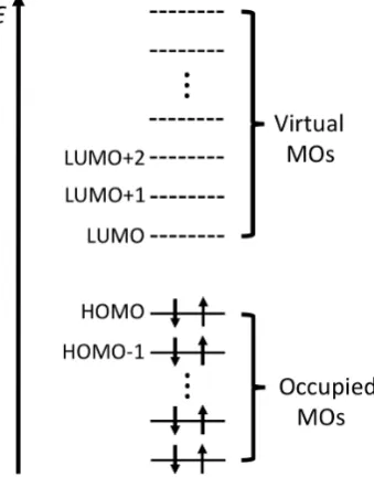
The resulting orbital picture is sketched in Fig. 1.3, where the MOs of an RHF

calculation for a closed-shell 2n-electron system are ordered according to their orbital

energies. Following the aufbau protocol the 2nlowest energy MOs are used to form the

new density matrices at step (5).

Once the calculation is converged, the orbitals which are occupied are called (guess

what!) the occupied orbitals, while the remaining, unoccupied MOs are the virtual

orbitals (or simply virtuals). The highest energy occupied MO is known as the Highest

Occupied Molecular Orbital (HOMO) and the lowest energy virtual is the Lowest

Unoccupied Molecular Orbital (LUMO). We will see soon that virtual MOs play an

important role in correlated methods.

1.5.2 Electron Correlation

The HF method treats the electron-electron interaction using a mean-field approximation,

that is the interaction is accounted only in an average fashion. In a large basis set

HF accounts for 99% of the total energy of a system, however it turns out that the

remaining 1% is extremely important for describing its chemistry.

The di↵erence between the exact non-relativistic energy of a system,Eexact, and the

restricted Hartree-Fock energy ERHF obtained in the limit that the basis set approaches

completeness was defined by L¨owdin in 1959 [32] as the correlation energy

Ecorr=Eexact ERHF (5.93)

This energy is due to a specific kind of correlation (Coulomb correlation) of the

electrons, which is not taken into account by the HF potential _VHF in Eq. (5.55). In

fact, quoting L¨owdin,[33] between two electrons “iand j there is in reality a potential

Hij which, particularly for small distances rij ⇡0, may be tremendously large. If this

potential is repulsive, like the Coulomb potentialHij =e2/rij, it tries naturally to keep

the particles apart, and, since this correlation is entirely neglected in forming the Slater

determinant, the corresponding energy is a↵ected by an error which is usually called

the ‘correlation energy’.”

(48)

1. Coulomb correlation: as just highlighted by L¨owdin’s quote, there is a Coulomb

interaction between the electrons that generally decreases the probability of finding

two electrons (of any spin) close to each other. Thus, for each couple of electrons

“i” and “j” the correct wave function must be such that its ij-pair probability

density

⇢ij(ri,rj) =

Z

(x1, . . . ,xn)† (x1, . . . ,xn)dx1. . . dxi 1dsi. . . dxj 1dsj. . . dxn (5.94)

is zero at their coalescence point, that is

lim

rij!0

⇢ij(ri,rj) = 0 (5.95)

This depression in the pair probability density is called theCoulomb hole and it is

at the origin of the famous and paramount electron-electron coalescence conditions

derived by Kato in 1957.[17]

2. Fermi correlation: electrons are indistinguishable and obey Fermi-Dirac

statis-tics, which imposes the antisymmetry requirement to the wave function. This

implies that two same-spin electrons cannot be found simultaneously at the same

point in space and consequently that the probability of finding one in the

immedi-ate vicinity of the other is close to zero. In this sense the correct wave function is

such that its pair probability density exhibits a “hole”, the Fermi hole.

Fermi correlation is taken into account “automatically” by using Slater determinants.

Thus, the correlation energy in Eq. (5.93) refers only to Coulomb correlation.

A minor distinction is worth making betweensame-spin correlation and

opposite-spin correlation. Same-spin correlation is the Coulomb correlation between electrons

having the same spin (not to be mistaken for Fermi correlation). Instead, opposite-spin

correlation is between electrons having opposite spin. Since the mathematics of a Slater

determinant is such that same-spin electrons are already “kept apart”, the contribution

to the correlation energy Ecorr due to same-spin correlation is usually minor and its

(49)

Another distinction is between dynamic and static correlation. Dynamic correlation

is associated with an instantaneous repulsion between the electrons, such as those

occupying either the same MOs or nearly spatially equal MOs. The static correlation

is usually associated with electrons avoiding each other on a permanent basis, such as

those occupying two energetically degenerate orbitals with di↵erent spatial distributions.

A typical example of where static correlation is very significant is bond breaking.

Eventually, the distinction between static and dynamic correlation remains nebulous

and mathematically not well-defined.

The coming sections dedicated to wave-function methods will be dealing with

“correlated methods”, that is methods which take into account either partially or fully

electronic correlation.

Unrestricted Hartree-Fock, correlation and spin contamination

Before proceeding with the established correlated methods, it is worth making a note on

the correlation problem in the context of unrestricted Hartree-Fock theory. A well-known

observation is that RHF cannot properly describe the bond breakage as it usually yields

wrong dissociation limits, that is the RHF energy of the system, close to dissociation,

is larger than the sum of energies of the isolated component molecules. On the other

hand, UHF is known to correctly model dissociation.

This success of UHF is due to the fact that the↵ and MOs involved into the bond

are not constrained to be spatially degenerate. As the bond is stretched the MOs break

their spatial degeneracy allowing for the localisation of the electrons on the molecular

fragments. Since the electronic localisation is energetically favourable during the bond

breakage, this event is associated with a lowering of the UHF energy below the RHF

one. The point where the RHF and UHF descriptions start to di↵er is often referred to

as a RHF/UHF instability point.

Since, in this situation, the UHF energy is lower than the RHF one, according to

definition (5.93) the UHF wave function has partly introduced electron correlation.

However, this correlation comes with a price: spin contamination. Once the MOs spatial

symmetry is broken, the wave function is not a pure spin state anymore, but it is

(50)

inferred from the expectation value of the S2 operator, usually denoted by the symbol

hS2i. Its correct expectation value for a pure spin state is hS2i=Sz(Sz+ 1), that is 0

for a singlet, 0.75 for a doublet, 2 for a triplet, etc. An UHF singlet, for example, might

contain some amount of triplet, quintet and so on.

ThehS2i value of the UHF wave function can be calculated using the formula

hS2_i=Sz(Sz+ 1) +n

occ. X

ij

|h i↵| ji|2 (5.96)

from which it can be easily verified that the RHF wave function will always yield, for

example, pure singlet spin states.

1.5.3 Configuration Interaction

The HF method provides the energetically best single-determinant many-electron trial

wave function within aone-electron basis of atomic orbitals. As the size of the basis

set is increased up to its completeness, the lowest possible single-determinant energy,

known as the Hartree-Fock limit, is reached. No further amelioration is possible by

variation of the one-electron basis.

However, as previously discussed, a convergedn-electron closed-shell RHF calculation

within anN-dimensional basis set yields N MOs, of which nare doubly occupied and

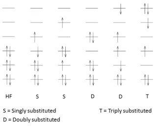
the remaining (N n) virtuals are left unoccupied. As sketched in Fig. 1.4, from

theseN converged MOs, a set of additionalh N_n 1iorthonormal Slater determinants

can be constructed by promotion of a number of electrons from the occupied to the

virtual MOs. Determinants which are obtained by promoting one, two, three, . . . , n

electrons in this way are namedsingly,doubly,triply, . . . ,n-tuply substituted (or excited)

(51)

[image:51.595.158.473.105.365.2]

Figure 1.4: MO diagram for HF and substituted determinants.

In the Configuration Interaction (CI) method, which was devised by Condon in

1930,[34] the many-electron basis for the trial wave function is systematically improved

by linearly combining the reference wave function 0 (usually the HF ground state

determinant) with a certain number of substituted determinants

˜ CI_⌘_c₀ ₀₊X

ir

cr_i r_i +X

i<j r<s

crs_ij rs_ij +_{· · ·} (5.97)

where the c0, cri, crsij, . . . , coefficients are the so-called CI amplitudes, ri are singly

substituted determinants in which an electron has been promoted from thereference

state occupied MO i to the virtual MO r, rsij are doubly substituted determinants

and so forth.

Since the CI wavefunction is just a linear combination of Slater determinants, the

TISE can be solved in this basis by following the “linear variational method” described

in Section 1.3.2, that is by diagonalization of the Hamiltonian matrixH as defined in

Eq. (3.24).

(52)

is referred to as CI-Singles (CIS), if it includes all the singly and doubly substituted

determinant CI-Singles-Doubles (CISD) and so forth, up to when all possible substituted

determinants are incorporated to form the so-called Full CI (FCI) wave function.

The FCI solution yields the best possible solution within a given one-electron basis.

To be more specific it recovers the maximum amount of correlation energy within the

basis set. Furthermore, as the size N of the basis set increases the resulting

many-electron basis of substituted determinants approaches completeness. It can be shown

that, in the limit N _{! 1}, that is for a sufficiently large one-electron basis, the FCI

wave function converges to theexact solution of the TISE.

Figure 1.5: CI convergence to the exact solution.

In this sense, the major advantage of CI over other correlated methods is that it

o↵ers a systematic manner to improve the accuracy of the trial wave function towards

exactitude. However, accuracy in CI comes at an high price. In fact, it can be shown

that a CI which includes up to m-tuply substituted determinant scales as

O(nmV2+m) =

8 > < > :

O N2m+2 if n⇡V >> m

O Nm+2 _if _{V >> n, m}

(5.98)

where nis the number of electrons, N is the size of the one-electron basis andV is the

(53)

CISDTQ scale as _O(N4),_O(N6) and_O(N10), respectively, for typical cases.

When the level of electron promotion m becomes comparable with the size of the

basisN, that is for FCI or nearly FCI, the computational scaling becomes_O(Ndetn2N2),

where Ndet is the product of the number of determinants for the alpha and beta

electrons separately. Thus, for a system with kalpha and kbeta electrons, where kis a

large number, the following number of determinants can be obtained via the Stirling

approximation for factorials

Ndet(N = 2k)⇡

16k

k⇡ k large (5.99)

This exponential scaling makes FCI unrealistic except for quite small molecules.

Furthermore, even if the truncated versions (CISD, CISDT, etc.) formally are much

lower scaling, these methods violate bothsize-consistency,[35] which establishes that

the energy of a system should equal the energy sum of the separate subsystems at the

bond dissociation limit, and the more generalsize-extensivity requirement,[36] for which

the energy should scale linearly with the number of particles in the system.

It is in this necessity of size-extensivity that the next wave-function method finds

its origin.

1.5.4 Coupled Cluster

The Coupled-Cluster (CC) set of methods stems from a motivation to find an improved

theory to truncated CI theory which is inherently size-extensive. It invokes a non-linear

expansion of the wave function, which defines a set of non-linear partial di↵erential

equations that need to be solved using iterative techniques. For this reason, CC theory

is much more involved than the linear expansion analogue of configuration interaction.

Since its introduction, first in nuclear physics[37] and then into quantum chemistry

in 1966 by Cizek,[38] CC has established its status as perhaps the most reliable yet

computationally a↵ordable approximation to the full CI expansion.

Single-Determinant Theory of Electronic Excited States and Many-Electron Integrals for Explicitly Correlated