THE STRUCTURE AND CONTENT OF GLOBULAR CLUSTERS
Gary S. Da Costa
July 1977
A thesis submitted for the degree of Doctor of Philosophy
It is a pleasure to thank my supervisor Dr Ken Freeman not only for his encouragement and assistance throughout the course of this work but also for giving freely of his time for discussion . and advice.
I am grateful also to Dr Russell Cannon and Dr Tim Hawarden of the UK Schmidt Telescope Unit for arranging the taking of plates for me with the 1.2m Schmidt ,telescope at Siding Spring Observatory. Dr J.E. Hesser and Dr S.W. Lee communicated details of their
photoelectric sequences in advance of publication for which I am most grateful. I am also most grateful to Dr Barry Newell for his
assistance both in obtaining and reducing the PDS data.
It is · also a pleasure to acknowledge many valuable discussions with the staff and students of Mt Stromlo Observatory particularly with Professor S.C.B. Gascoigne and Drs J.E. Norris, E.B. Newell and A.W. Rodgers. I would also like to acknowledge useful correspondence with Dr G. Illingworth and Professor S. van den Bergh.
The use of the facilities of Mt Stromlo and Siding Spring Observatory and the assistance of the maintenance staff is also
gratefully acknowledged. I am indebted to the Director of the Anglo-Australian Observatory for allowing me to use the PDS microdensitometer and to the staff of the Computer Centre of the Australian National
University for their assistance.
Brigitte Coles, Sandy Dabb and Suad Khouri deserve special
thanks for their careful typing of this thesis; special thanks also to Mark Burke for drawing the diagrams and to Keith Smith for photographing and reducing the computer generated plots.
A detailed study has been made of the structure and stellar content of the nearby southern globular clusters NGC 104 (47 Tue), NGC 6397 and NGC 6752. Accurate surface brightness profiles have been derived for each cluster and star counts made from plates taken with lm, 1.2m Schmidt and 4m telescopes. Because of the proximity of these clusters, it is possible to determine from the star counts the number and distribution with radius of stars with masses as low as one half the giant star mass. For NGC 104 the count data show a clear difference in distribution between the upper main sequence stars and stars of lower mass consistent with a tendency towards equipartition of energy.
A system incorporating a TV detector for the measurement of accurate radial velocities of faint stars has also been developed, and used to determine a line of sight velocity dispersion for NGC 6397.
These observational data have then been combined with dynamical models to investigate the structure of the clusters. The models are based on isotropic lowered Gaussian velocity distribution functions,
are spatially limited and include a realistic range of stellar masses. The distribution functions for each mass are related by an expression which would correspond to equipartition of energy in the absence of a finite velocity cutoff. In general the agreement between the model predictions and the observational data is good. In particular, it appears that the limiting radius is the same for stars of different mass as required by a tidal cutoff. However, for NGC 104 the
stars than th e nwnber expected from the Salpeter function. A model in which the ' equipartition of energy' condition is modified however, does not need any enhancement of remnant stars to reproduce the
observed central . velocity dispersion. A lower limit to the total mass and mass to light ratio of each cluster is given.
The models and the star counts are also used to investigate the mass function for the stars still on the main sequence in each cluster. The data agree well with a power law dN cr m -(l+x) dm and upper and lower limits are placed on the present value of
x
in each cluster. Large differences exist between the clusters with NGC 104 containing significantly more low mass stars than NGC 6752 which in turn contains more than NGC 6397. The origin of these differences is investigated and i t is concluded that they cannot have resulted from dynamical evolution alone. The initial mass functions of the clusters must also have been different. Evidence is presented toCHAPTER I 1.1 1.2
l._3
CHAPTER II
INTRODUCTION AND THESIS OUTLINE Introduction
Discussion of Previous Work
(a) The Stellar Content qf Globular Clusters (b) The Structure of Globular Clusters
Thesis Outline
DYNAMICAL MODELS OF GLOBULAR CLUSTERS 2.1 Introduction
2.2 Model Theory
2 .3 Numerical Techniques
2.4 Model Construction Method (a) Initial Procedures
(b) Inclusion of Remnant Stars (c) Calculation of the Model
(d) Conversion to Dimensional Quantities (e) Comparison with Observations
2.5 Summary
CHAPTER III OBSERVATIONAL METHODS AND RESULTS · 3 .1
3.2
3 . 3
Introduction
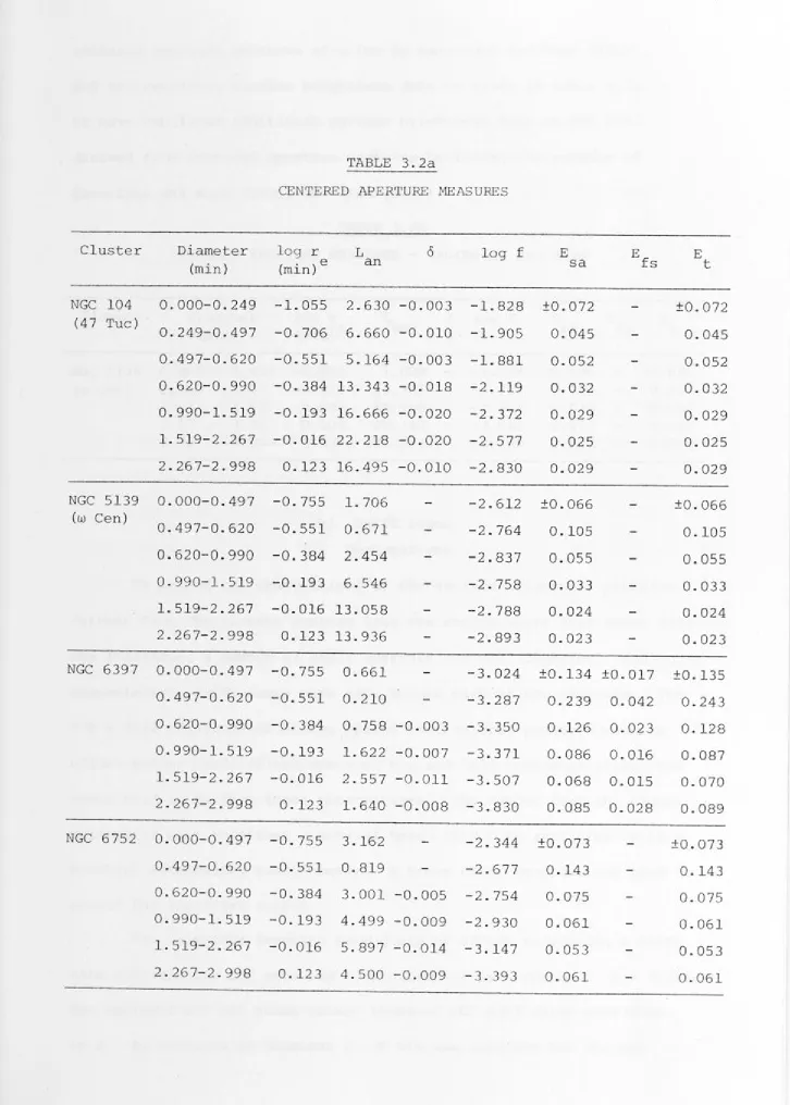
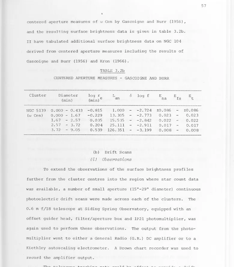
Surface Brightness Profiles (a) Centered Aperture Measures
(i) Observations (ii) Reductions (iii) Errors (b) Drift Scans
(i) Observations (ii) Reductions (iii) Errors (c) Results
Star Counts (a) Observations
3.4
CHAPTER IV 4.1 4.2 4.3 4.4
CHAPTER V
(ii) Crowding Corrections and Errors (d) Limiting Magnitude Determinations (e ) Re sults
Radial Velocity Measurements
(a) System and Re duction Technique Description (b) Velocity Dispersion of NGC 6397
THE STRUCTURE OF GLOBULAR CLUSTERS Introduction
Models of NGC 104
Models of NGC 6397 and NGC 6752 Discussion
THE MASS FUNCTION OF GLOBULAR CLUSTERS
88 112 1 2 1 141 141 143
148 148 167 175
5.1 Introduction 181
5.2 The Present Mass Functions of NGC 104, NGC 6397 and 181 NGC 6752
5.3 Discussion 189
(a) The Effects of Dynamical Evolution (b) The Initial Mass Functions
(c) The Origin of the Different IMFs .
FUTURE WORK
BIBLIOGRAPHY
190 196 202
210
Table
1.1 Basic Cluster Data
3.1 Colours and Magnitudes Through Centered Apertures 3.2a-b Surface Brightness Results from Centered
Aperture Measures
3.3a-e Surface Brightness Results from Drift Scans
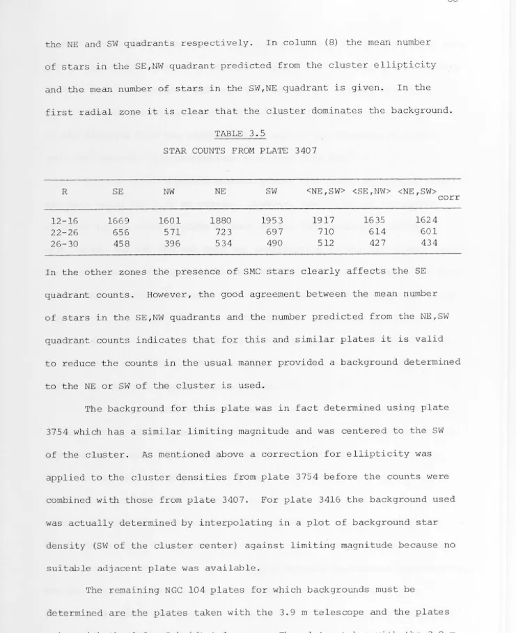
3.4 Star Counts Used in Surface Brightness Profiles 3.5 Quadrant Data from Count of Plate 3407
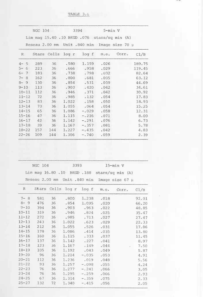
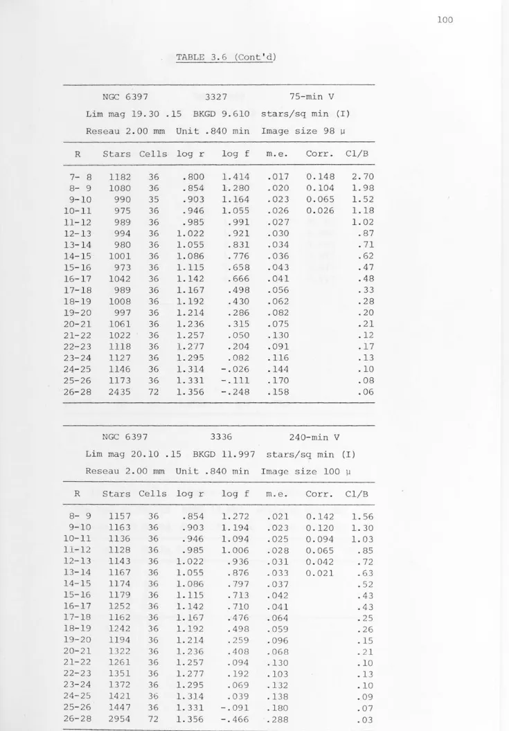
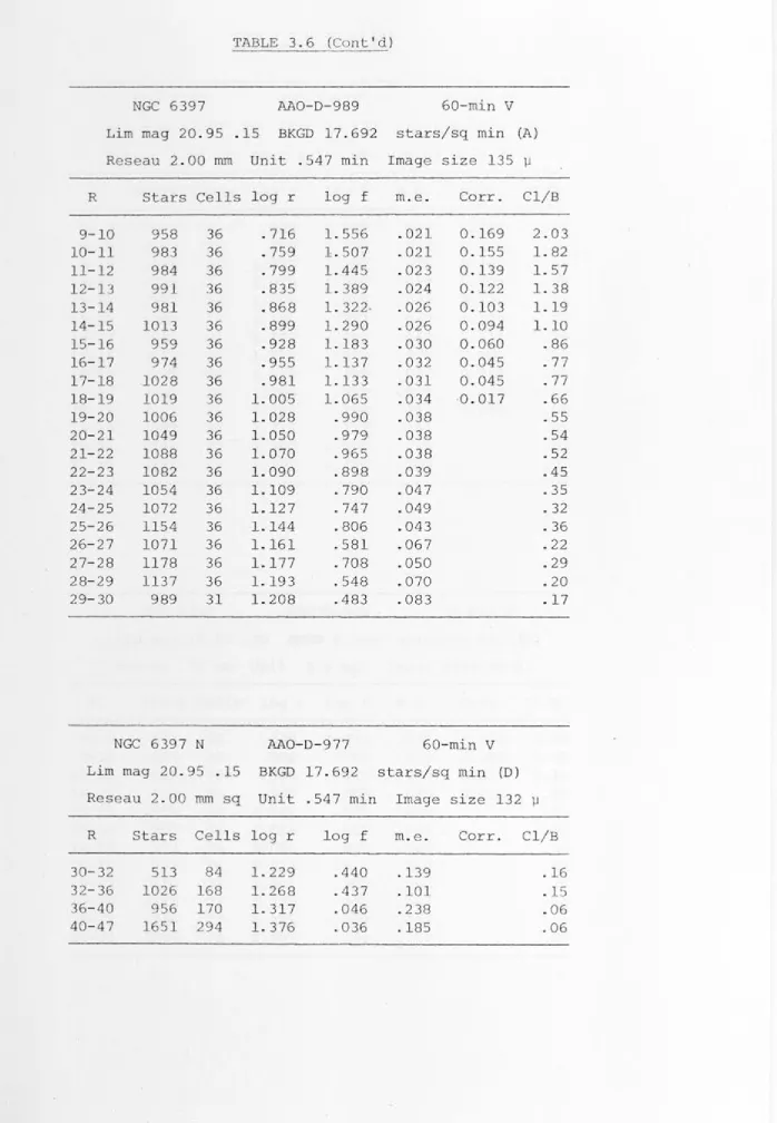
3.6 Star Count Data
3.7 NGC 6397 Limiting Magnitude Determinations 3.8 Distances and Distance Moduli
3.9 Cumulative Luminosity Function Data 3.10 Radial Velocities of Stars in NGC 6397
4.1 NGC 104 Mass Classes
4.2 Parameters of NGC 104 Models 4.3 NGC 6397 Mass Classes
4.4 NGC 6752 Mass Classes
4.5 Parameters of NGC 6397 and NGC 6752 Models 4.6 Total Mass and Mass to Luminosity Ratio Limits
5.1 Values of
x
for NGC 104 Remnant Enhancement 5.2 Dynamical Evolution Timescales5.3 Estimated Fractions of Initial Total Mass
Page 18
51 56
62 . 65 86 92 120 126 128 145
149 165 168 169 173 180
Figure 2.1 3.la-d 3.2a-b 3.3 3.4 3.5a-c 3.6a-b 3.7 3.8 3.9a-c
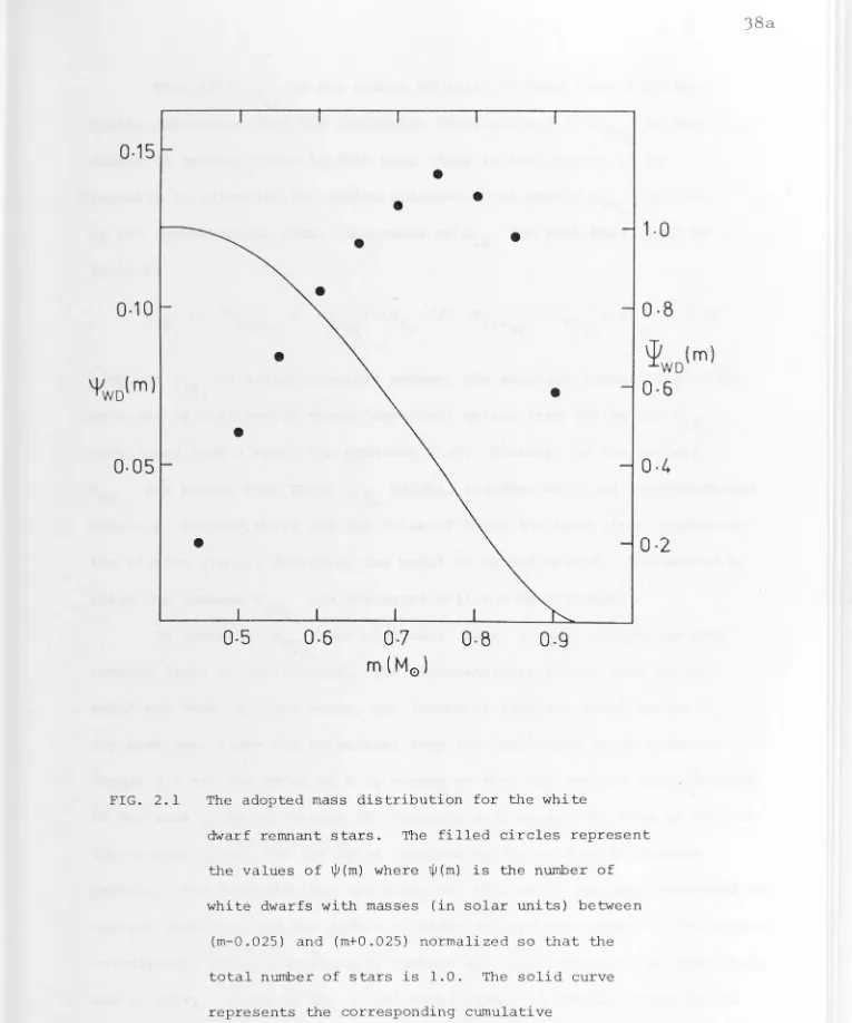
Adopted White Dwarf Mass Distribution
Surface Brightness Profiles for NGC 104, NGC 5139, NGC 6397 and NGC 6752
Surface Brightness Profiles for NGC 5272 (M3) and NGC 6341 (M92)
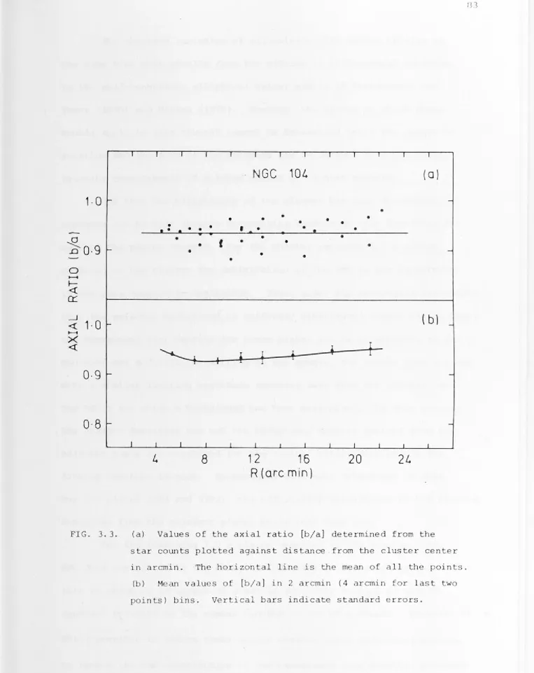
Ellipticity of NGC 104
Comparison of Crowding Corrected and Uncorrected Densities with Densities Requiring no Correction Star Density for NGC 104, NGC 6397 and NGC 6752 VPDS' VPE Relation for Stars Measured in NGC 121 and NGC 6752
VPDS' VPE Relation for Stars Measured in NGC 6397 Comparison of Distribution of Stars of Different Mass in NGC 104
Cumulative Luminosity Functions for NGC 104, NGC 6397 and NGC 6752
3.lOa-c Differential Luminosity Functions for NGC 104, NGC 6397 and NGC 6752
Page
JSa
67 72 83 89 109 116 118 123 130 134 3.11 Comparison of the Luminosity Functions of figs. 3.lOa-c 1384.1 Comparison of NGC 104 Model 1 with the Observational
Data 151
4.2 Comparison of NGC 104 Model 2 with the . Observational
Data 154
4.3 Comparison of NGC 104 Model 3 with the Observational
Data 157
4.4 Comparison of NGC 104 Model 4 with the Observational
Data 159
4.5 Comparison of NGC 104 Model 5 with the Observational
Data 162
4.6 B-V versus Radial Distance for NGC 104 Model 2 166 4.7a-b Comparison of Model of NGC 6397 and NGC 6752 with the
Observational Data 170
OIAPTER I
INTRODUCTION AND THESIS OUTLINE ·
1.1 INTRODUCTION
Globular clusters have long been objects of astronomical
interest. They are evidently amongst the oldest objects in the galaxy, and so determinations of their stellar content may yield information on star formation processes early in the lifetime of our galaxy. Further, their colour-magnitude diagrams and giant branch luminosity functions
place important constraints on stellar evolution theories for population II stars. In addition, because of their richness and symmetry i t is
natural to look to theories of stellar dynamics to explain their overall structure.
Indeed the structure and stellar content of globular clusters are inextricably interwoven ; the cluster giants and subgiants, whose
distribution is mostly easily measured, contribute almost all the visible light output of a cluster while stars of lower m~ss presumably contribute most of the total mass and dominate the gravitational field in which the bright stars move. If there i -s any tendency towards equipartition of energy, then the relative number of low mass stars will increase with distance from the cluster center and a dynamical model will be needed to estimate the correct populations of s 'tars of different mass in the
cluster as a whole. Further i t is possible that significant numbers of stars will have escaped from a cluster over its lifetime and so in order to relate the present mass function of a cluster to the initial mass
The principal aim of this thesis concerns both th e se areas of interest: by gathering sufficient observation al material on a small number of nearby clusters, an attempt will be made to provide some understandin·g of the structure and stellar content of globular
clusters. However, before describing the procedures to be followed
in this task, a discussion of previous work in these areas is presented.
1.2 DISCUSSION OF PREVIOUS WORK
(a) Stellar content of globular clusters
Observational work on the stellar content of globular clusters has generally proceeded along one of two possible approaches: either the stellar content has been directly determined from luminosity functions, or i t has been inferred from measured velocity dispersions which yield total masses and mass· to light ratios. Luminosity functions have been published for a number of clusters (e.g. Sandage 1954, 1957, S imoda
and Fukuoka 1976 for M3; Tayler 1954, Hartwick 1970, van den Bergh 1975, Fukuoka and Simoda 1976 for M92; Simoda and Tanikawa 1972 for MS and Ml3; Sandage, Katem and Kristian 1968 for Ml5; Dickens and Woolley 1967 for
w
Cen; Lee 1977, Hesser and Hartwick 1977 for 47 Tue) but with the exception of the results of van den Bergh (1975) these luminosityfunctions do not reach absolute magnitudes much fainter than those of the main sequence turnoff. Hence, although these luminosity functions are useful for helium abundance determinations and for testing the detailed predictions of theoretical calculations of giant branch evolution, the stars observed are all of approximately the same mass and so they yield little information on the mass functions of the
magnitudes fainter than V
=
23 mag, has shown that the number of stars per magnitude interval in this cluster does not appear to increase forabsolute magnitudes fainter t h a n ~ ~ + 6 down to the limit of the data a t ~~ + 8. This may indicate that the present mass function of this cluster does not contain large numbers of low mass stars, although the stars at the limit of the obseryational data have masses only of the order of one half that of the cluster giants. I t is clear then, that the number and distribution with radius of stars with masses appreciably less than that of the cluster giants can only be studied in this way in the most nearby clusters.
However, using the alternative approach mentioned above, i t is possible to gain some information on the low mass star content of
globular clusters. The earliest detailed results using this approach are those of Wilson and Coffeen (1954). These authors measured line of sight velocities for fifteen bright giants in M92 and determined a line of sight velocity dispersion <v 2>~
=
4.4 kms-l from the moduli of ther
deviations of the individual ·stellar velocities from the mean. Then using a form of the viria_l theorem given by Kurth ( 19 50) , they obtained a mass of 3.3 x 10⁵M for the cluster and a mass to light ratio (M/L)
0
=
2.0 in solar units.These results however, were modified by Schwarzschild and
Bernstein (1955) who used an improved form of the virial theorem given 5
by Schwarzschild (1954) to derive a mass of 1.4 + 1.0 x 10 M and
0
Some years later Feast and Thackeray (1960) reanalyzed the data of Wilson and Coffeen (1954) using, instead of the moduli, the squares of the deviations from the mean velocity. Combining this with a
different treatment of the effect of observational errors on the observed dispersion, they obtained a new value for the velocity
5
dispersion of M92 and from i t a mass of 1.8
+
1.2 x 10 M and an (M/L)0
=
1.0+
0.7 (solar units). The form of the virial theorem given by Schwarzschild (1954) was again used. Feast and Thackeray (1960) also attempted to determine the line of sight velocity dispersion of 47 Tue(NGC 104) but because of an unexplained dependence of the measured
velocities on spectral type , only upper limits to the mass and mass to light ratio of the cluster were determined. Even so, this upper limit to the mass the light ratio was low (0.3
+
0.4 solar units), againpointing to apparent differences between the stellar populations of globular clusters and elliptical galaxies .
. The interpretation of these mass to light ratios for globular clusters was advanced by the results of Sandage (1957). He extrapolated his observed luminosity function (for stars brighter than M
z
+
6.5). V
for M3 to fainter magnitudes using a combination of the (normalized)
luminosity functions of van Rhijn (1936), Luyten (1939) and Kuiper (1942). Then, by considering the probable number and mass of white dwarfs
present and by using the mass-luminosity calibration of Kuiper (1938, 1942) he derived a mass to luminosity ratio consistent with the M/L value for M92 given by Schwarzschild and Bernstein (1955).
the dispersion in one coordinate so a value for the ratio <v2>/<v r 2> must be assumed; usually <v2> is taken as three times <v 2> which
r
corresponds to an isotropic velocity distribution. Further, the virial theorem requires a value of <v2> appropriate for all stars. The
measured value however, usually applies only to the brighter stars in the cluster and the fainter, less massive stars, which presumably
contribute most of the mass of the cluster, will generally have higher
velocity dispersions i f there is any tendency towards equipartition of
energy. An additional complication is that the velocity dispersion must decrease with radius because of the existence of a finite boundary to
the cluster. Hence, i t is clear that the measured velocity dispersion
will depend on the positions in the cluster of the stars observed.
The kinetic energy of systematic motions such as rotation must also be
included. The potential energy, on the other hand, is usually determined from the distribution of the bright stars, either from the surface
brightness profile or directly from star counts. In either case the
derived potential energy will be incorrect i f the distribution of the
bright stars differs from that of the lower mass stars which determine
the mass distribution. Fortunately however, some of these difficulties
and uncertainties can be overcome i f the measured velocity dispersion
is used in conjunction with a dynamical model to estimate the total mass
and mass to light ratio of a cluster.
Harding (1965) measured line of sight velocities for 31 members
of the globular cluster
w
Cen. From these stars, 13 were selected ashaving large rotation moment, and were observed repeatedly to enable accurate d e terminations of their line of sight velocities . Th e se
velocities we re then used to d e termine the internal rotation of the
individual velocities and the mean were consistent with solid body rotation (within the region containing the observed stars); the
velocity dispersion of the measured stars, relative to this rotation
2 ~ -1.
law, was <v >2
=
5.8+
3.8 kms These results were then used by rDickens and Woolley (1967) to derive a total mass and mass to light ratio for this cluster. Unlike the previous results however, these estimates were based on a dynamical model of the cluster rather than on the virial theorem.
From their extensive compilation of data on
w
Cen, Dickens and Woolley (1967) determined,inter al-ia,
the mean projected densitydistribution for stars brighter than M ~
+
2 as a function of distanceV
from the cluster center. They then deprojected this observed data and normalized so that the central (space) density was unity. Models based on a variety of assumptions were then calculated and the model densities
compared with the observed densities. A best fit was found for a model calculated with a truncated Maxwellian distribution, a continuous
distribution of stellar masses and equipartition of energy. From the fit of this model to the observational data a l~ngth scale in dimensional units was determined. Then by combining this length scale with the
velocity dispersion given by Harding (1965) the central density of the cluster in physical units was found. Once this central density had been determined, the total mass of the cluster was obtained by integrating the dimensionless model density. Using these techniques, Dickens and Woolley give the total mass of
w
Cen as 7 x 10⁵M and derive a mass to light0
ratio of 0.5 in solar units.
However, these values have been seriously questioned by Poveda and Allen (1975) who noted that the models constructed by Dickens and Woolley
Further, they drew attention to the fact the velocity dispersion used by Dickens and Woolley (1967) to derive the central density of
w
Cen was the velocity dispersion relative to the local rotation law ratherthan the velocity dispersion relative to the mean velocity of the cluster. Hence the contribution of the rotational energy to the maintenance
of the cluster structure was neg-lected. They then went on to estimate more realistic lower limits to the mass of
w
Cen by three separatemethods; by - using the method of Dickens and Woolley (1967) but using a total velocity dispersion (calculated from the line of sight velocities measured by Harding 1965) rather the velocity dispersion relative to the rotation
law; by a method based on the observed rotation curve; and by the
virial theorem . These three estimates agreed remarkedly well and they indicate that the mass of
w
Cen exceeds 3.3 x 10⁶M and that (M/L) > 3o
Vfor this cluster . Poveda and Allen (1975) point out that this mass to light ratio is similar to that for the solar vicinity (M/L) "" "" 2.2
pg and to that for a cylinder perpendicular to the galactic plane (M/L)
pg "" "" 3.4
-
3 . 8 (Oort 1965) .The most recent observational work on the stellar content of globular clusters is that of Illingworth (1975, 1976) who derived total masses and mass to luminosity ratios for ten centrally concentrated
globular clusters from measurements of their surface brightness profiles and
central
velocity dispersions. The surface brightness profilesregions of the clusters)· and the dimensionless total masses of the models, which depend only on the ratio of the tidal radius to the core radius to derive the total masses of the clusters. These total
masses, together with the absolute magnitudes of the clusters, then yield estimates of the mass to light ratios. Values of (M/L)
V ranging from 0.9 to 2.9 were found, with a mean value of 1.6
(Illingworth 1976).
The implications of these observationally determined mass to light ratios were then investigated (Illingworth 1975). Firstly, the luminosity functions for M3 (Sandage 1954, 1957) and MS (Simoda and Tanikawa 1972) were extrapolated to fainter magnitudes using the solar
neighbourhood luminosity function given by Wielen (1973). A
mass-luminosity calibration was then determined and the (M/L) value for each of the luminosity functions calculated. Remnant stars were also
included in the calculation: their number was estimated by fitting the Sandage - (1957) modified Salpeter (1955) initial luminosity function at
the turnoff point with all stars more massive than the current turnoff mass assumed to have become 0.6M white dwarfs . . These calculated (M/L)
0
values agreed reasonably well with the observed values while mass to luminosity ratios calculated on the basis of different extrapolations did not. This result was taken to indicate that low mass stars
constitute a large proportion of the present stellar content of these clusters (Illingworth 1975). However, these results again depend on the assumption that the mass to light ratio does not vary with distance from the center in a globular cluster and hence are still relatively uncertain.
The first of these is dynamical relaxation through two body encounters which leads to a gradual evaporation of stars from the cluster. The
second is the effect of the compressive gravitational shocks which occur each time the cluster passes through the galactic plane. The term
'shock' is used because in the outer regions of a cluster, the orbital period of a star is usually long compared to the time of passage through
the galactic plane.
The effects of these gravitational shocks have been considered by Ostriker
et al .
(1972). They showed that provided the orbital period of a star in the cluster is long compared with the time of passage through the galactic disk, its increase in velocity can be calculated using an impulsive approximation and an increase in the random kinetic energy of the cluster results. The gain in kinetic energy or 'shock heating' is largest for the stars furthest from the cluster center and since, · if there is any tendency towards equipartition of energy these stars will have generally lower masses, these authors suggest that this processleads to preferential loss of low mass stars from globular clusters.
Indeed, they have gone on to suggest that globulpr clusters are strongly deficient in low mass stars and that an appreciable fraction of the halo population consists of escaped globular cluster stars. Clearly
observational evidence which yields information on this suggestion would be of great interest.
(b) The structure of globular clusters
since the time of relaxation at the center of a globular cluster is usually a small fraction of its age (e.g. Peterson and King 1975) that stellar encounters have strongly influenced the form of the velocity distribution function. An explicit form of this function, expressed in terms of the integrals of motion of a star, is then assumed and the spatial characteristics of the JnOdel determined by solving Poisson •·s equation. This approach has been followed by many authors (e.g.
Chandrase khar 1960; Woolley 1954; Woolley and Robertson 1956; Woolley and Dickens 1961; Spitzer and Harm 1958; Oort and van Herk 1959; Michie 1963a,b; Michie and Bodenheimer 1963; King 1966a; Prendergast and Torner 1970;
Prata 197la,b; Wilson 1975; Da Costa and Freeman 1976) each of which assumed different forms for the velocity distribution function.
Of these studies perhaps the most detailed, in terms of comparing model predictions with the observations of real globular clusters, are
those of Oort and van Herk (1959), King (1966a) and Da Costa and Freeman (1976) . · In their study of the structure and dynamics of M3, Oort and van Herk (1959) used the star counts to different limiting magnitudes from which Sandage (1954) had derived a luminosity function, star counts by von Zeipel (1908, 1913) and surface brightness measures by Hertzsprung
(1918) to constrain their models of this cluster. They considered that the changes in slope (in a surface density versus radius plot) for counts with limiting magnitudes fainter than the main sequence turnoff (i.e.
counts with smaller mass limits) indicated equipartition of energy in the cluster. This assumption, combined with a calculation of relaxation
times at various radii and the apparently smooth variation of density with radius , led them to assume an anisotropic velocity distribution
predominantly radial velocities at large distances from the center. I t was truncated sharply at the escape velocity. These authors then constructed a variety of models based on this velocity distribution, incorporating different assumptions for the number and mass of the remnant stars and for the form of the luminosity function of the low mass stars. A best fit between the model densities and the observed densities (whiw½ had been converted to space densities) was found for a model in which the number of low mass stars was considerably less than
that predicted from the van Rhijn (19 36) luminosity function and in which the number and mass of white dwarf stars was assumed to equal the
number and mass of stars brighter than M
=
+
3 . 5 in the cluster.V
5
This model had a total mass of 1.5 x 10 M with a mass to light ratio of
0
approximately 0.25 (solar units). However, since recent results indicate that the shock heating which occurs each time the cluster crosses the
galactic plane has a strong randomizing influence on stellar orbits in the outer regions of a cluster (Keenan and Innanen 1975, Henon 1971, Prata 1971b, Spitzer and Chevalier 1973), i t is likely that some of the
assumptions, particularly the assumption of an ~nisotropic velocity
distribution function made by Oort and van Herk (1959) may not be valid. Hence their estimates of the mass and mass to light ratio for M3 are rather uncertain.
The understanding of the structure of globular clusters was advanced by King (1962) who demonstrated that a cluster possesses a finite boundary. He identified this boundary with the tidal cutoff
imposed by the gravitational field of the galaxy (predicted theoretically by von Hoerner 1957) and went on to show that an individual cluster could be described by three parameters; a richness factor, a 'core' radius and
radius measuring the central concentration of the cluster. Since physically a cluster is described by a total mass and a total energy in a tidal gravitational field of a certain strength, King (1962) concluded that globular clusters are as similar in structure as possible .
In a later paper (King 1~66a) these results were used as a basis for a theoretical treatment of the structure of globular clusters.
Because of the short relaxation times at the center of a cluster, King (1966a) suggested, as had others before him, that the velocity distribution at the center of a cluster should have a form produced by stellar encounters. Yet because the galactic tidal field limits the radius of the cluster, he pointed out that this distribution function should go to zero at the velocity needed to reach the cluster boundary rather than at the velocity for escape to infinity. These requirements are described by the steady-state Fokker-Planck equation subject to a finite velocity cutoff (e.g. Spitzer and Harm 1958) and a lowered Gaussian function, i.e. a Maxwellian minus a constant, is an analytic approximation (Michie 1963a, King 1965) to its solution.
By assuming that this
isotropic
velocity distribution function applies throughout a cluster and that all the stars in the cluster have the same mass, King (1966a) went on to construct a one parameter set of spatially limited self-consistent models for globular clusters. The models were presented as a set of curves in which the logarithm of the normalized surface density is plotted against the logarithm of theradial distance expressed in terms bf the core radius since, as noted by King (1966a), projection of the model space densities onto the plane of
by its value of the central concentration parameter C; C is the logarithm of the ratio of the tidal radius to the core radius· of the curve.
Considering the simplicity of the models, the agreement between the model curves and available observational data is remarkedly good
(e.g. King 1966a, Illingworth and Illingworth 1976, Peterson 1976) over a large range of central concentrations. Indeed, these models have been used with extensive star count data (King
et al.
1968) to determine core radii, tidal radii and other structural parameters for . a large number of clusters (Peterson and King 1975, Peterson 1976).However, Da Costa and Freeman (1976) showed that no King (1966a) model gives a satisfactory fit to the observed surface brightness profile of the globular cluster M3. This profile, which covers five decades in intensity, was made up of unpublished electronographic measures by Kron and Hewitt, photoelectric measures by King (1966b) and star counts
from the compilation of King
et al.
(1968). To investigate the cause of this discrepancy these authors carried the models of King (1966a) one step further by relaxing the assumption that the stars in the cluster all have the same mass (see also Prata 197la,b). In these models the starsare grouped into a number of mass classes each of which is assumed to have a lowered Gaussian velocity distribution function. The distribution
functions are related by a condition which would correspond to equipartition of energy between stars of different mass in the absence of a finite
velocity cutoff.
The models were applied to M3 using the luminosity function given by Sandage (1954, 1957) extrapolated to fainter magnitudes with the
Salpeter (1955) initial luminosity function at the turnoff and assuming that all stars more massive than the current turnoff mass have become white dwarfs of mean mass 0.6M. I t was found that this type of
0
model gave an excellent fit to the surface brightness profile of this cluster. The total mass of the cluster model was 3.3 x 10 M, with a 5
0
mass to light ratio of 1.6 in solar units in good agreement with the mean value found by Illingworth (1976). However, despite the good agreement of this particular model with the available observations, i t is s t i l l true that at present, there is insufficient observational material to thoroughly test the validity of the assumptions on which this type of model is based. I t is one of the aims of this thesis to attempt to rectify this situation.
The second method of investigating the structure of globular clusters is to follow the dynamical evolution of model systems
numerically, either by direct N-body calculations or by Monte Carlo simulations. The major purposes of these type of calculations are to test the predictions of stellar dynamical theories for systems governed by two body encounters and to gain insight into the factors which
determine the evolution of such systems. In particular escape phenomena can be studied in detail. These subjects have been recently reviewed in detail (Aarseth and Lecar 1975, Spitzer 1975, Wielen 1975) and so only a summary of the results is given here. Original references for the
results quoted can be found in these review articles.
Because of the time consuming force calculations, investigations of stellar systems by direct numerical integration of the equations of motion of N bodies (the N-body problem) is practical only for relatively small (N ~ 500) values of N. However, for such systems there is
theories. Relaxation proceeds on timescales comparable with the theoretical two body encounter relaxation times and the velocity distribution becomes isotropic in the central regions independent of the initial conditions. Segregation of stars by mass occurs but because of finite velocities of escape full equipartion of energy is not
achieved. During the later stages of calculation, the core of the system is dominated by a close binary; this acts as an energy sink and has an
important effect on the dynamics of the system. In particular, the binary prevents the complete collapse of the core by ejecting stars. Escape
rates are found to be approximately independent of mass for all but the most massive stars which escape less frequently.
These calculations can be extended to larger values of N by making use of Monte Carlo simulation techniques if the same basic assumptions which underlie the use of the Fokker-Planck equation in stellar dynamics (i.e. that . the stellar system can be adequately
represented by a one-particle distribution function with evolution due only to binary encounters) are assumed to apply. The results for the Monte Carlo simulations are then very similar in most aspects to the N-body calculations and to the predictions of stellar dynamics theory. In particular, i t is found that the velocity distribution does indeed relax towards a Maxwellian minus a constant in the central regions of the system. Mass segregation occurs on timescales comparable with the
relaxation time of the system but the escape of stars in the absence of shock heating is approximately independent of mass. If shock heating is included then escape rates are increased and depend more strongly on mass since the low mass stars are generally further from the cluster
throughout the evolution of the system with the radius containing for example, 2% of the total mass of the cluster, going to zero in a finite time. I t is suggested however, that as for the N-body calculations this collapse might be halted by the formation of a close binary in the collapsing region which sinks to lower and lower energies ejecting other stars from the core.
In general following Spitzer (1975) i t appears that a wide range of evolutionary histories are possible for globular clusters. However, for most clusters the relaxation time is shorter than the age, so two occurrences seem likely. Firstly, i f a significant range of masses was initially present in the cluste.r then considerable mass
segregation should have occurred, with the majority of the low mass
stars far from the cluster center or removed from the cluster altogether if shock heating is non-negligible. Secondly, unless the formation of binaries intervenes to half the collapse, at least some clusters
should have gone through at least one phase of core collapse, whatever that may entail.
I t is clear then, in the light of the previous theoretical and observational work outlined above, that the time is ripe for a detailed study of the structure and stellar content of globular clusters. In particular answers should be sought for the following questions:
(b) Is the
pr es ent
mass function for stars still on the main sequence in globular clusters the - same in all clusters? If not, arethe differences due entirely to dynamical evolution or are differences in
initial
mass functions between clusters necessary?It is the purpose of this thesis to attempt to answer these questions. In the following section the procedures followed in this task are outlined.
1.3 THESIS OUTLINE
The first step in seeking the answers to the questions posed above is to select a small number of clusters for detailed study. Obviously because of the intrinsic faintness of the stars below the main sequence turnoff, such a study can be contemplated only for the very nearest of globular clusters. However, although this is the overriding selection criterion, other factors also influence the selection. I t is important that the clusters be at relatively high galactic latitudes to minimize as far as possible the field star back-ground level and the possibility of non-uniform absorption across the cluster. Further the clusters chosen should be relatively rich to reduce uncertainties due to sampling errors.
For these reasons the clusters chosen for detailed investigation in this thesis are NGC 104 (47 Tue), NGC 6397 and NGC 6752. The basic
data for . these clusters are given in table 1.1 and with the exception of the distance moduli which come from Hartwick and Hesser (1974), Cannon (1974) and Wesselink (1974) respectively, these data are taken
from Arp (1965). Briefly NGC 104 is a massive metal rich cluster while in contrast NGC 6397 is a very metal deficient cluster of faint
TABLE 1.1
BASIC CLUSTER DATA
Cluster Ct.
( 19 50)
8
( 19 50) 1
II bII
NGC 104
ooh 21~9 -72° 21 306° -45°
( 47 Tue)
NGC 6397 17h 361;18 -53° 39 339° -12°
19h 061;14 -60° 04
.
337° -26°NGC 6752
~
Cone. class
III
IX
VI
Sp. type
G3
FS
F6
V r_l (kms )
-24
+11
-39
(rn-M) app 'V
13.15
12.3
13.2
I-'
included in this study because i t is apparently the nearest globular cluster. The remaining cluster NGC 6752 is a typical halo cluster of intermediate metallicity and of 'average' absolute magnitude. I t is clear from the distance moduli given in this table that limiting
exposure plates taken on fine grain emulsions with the large telescopes now available in the southern he~sphere will reach stars with absolute magnitudes of approximately MV ~
+
10 in each of these clusters.Such stars have masses of approximately 0.45M (e.g. Veeder 1974), i.e.
0
masses of the order of half the giant star mass.
The remainder of this thesis is organized into chapters each of which is a separate step towards the fulfilment of the aims of the thesis.
In chapter II a detailed description of the theory underlying the models to be investigated is presented and discussed. The models are those
used by Da Costa and Freeman (1976) and have been mentioned briefly above. Also included in this chapter is an outline of the techniques used in
constructing a model or a particular cluster. Further, the observational data required to limit the range of possible cluster models are listed.
In Chapter III the methods used to obtain these observational data are described . Surface brightness profiles are determined for each cluster from centered aperture photometry and from small aperture drift scans. Star counts are also given and from these main sequence luminosity functions for particular regions in each cluster, and radial distributions of stars of different mass, are derived. The ellipticities of these clusters are also investigated. A system for measuring accurate radial velocities of faint stars is described and a line of sight
In Ch a pte r IV th e observ a ti o nal data and th e mo d e ls are combined to inve stigate the dynamical structure of th e cluste rs in this study. In g e ne ral the agree ment betwe e n the mode l pre dictions and the
observations is excellent for both the surface brightness profiles and the star count data. However, i t is found that for NGC 104 agreement between the observed central velocity" dispersion (Illingworth 1976) and
the model predicted central velocity dispersion is possible only i f the number of remnant stars is significantly more than the number expected from the Salpeter function. A further model of this cluster is
calculated in which the assumption of equipartition of energy is modified and i t is found that the increase in the number of remnant
stars is not necessary for the central velocity dispersion of this model to agree with the observed value. Lower limits to the total mass and mass to light ratio for each cluster are also given.
In Chapter V the stellar content of the clusters is investigated. The present mass function in each cluster is found to obey a power law of the form dN a m-(l+x) dm and with the aid of the star counts in the outer regions of the clusters and the models, upper and lower limits are placed on the present value of x in each cluster. Large differences are
found between the clusters in the sense that NGC 104 has more low mass stars than NGC 6752 which in turn has more than NGC 6397. The origin of these differences is investigated using the Monte Carlo simulation
models of Spitzer and Shull (1975) and i t is conclude d that the differences in th e prese nt mass functions canno t h a v e res ulte d fro m d ynamic a l
CHAPTER II
DYNAMICAL MODELS OF GLOBULAR CLUSTERS
2.1 INTRODUCTION
In this chapter a set of dynamical models for spherical star
clusters is described. The models are analogous to those of King (1966a) in that they are based on a velocity distribution function suggested by the short (in terms of the cluster age) stellar encounter relaxation times at the center of most clusters and by the existence of a finite cluster boundary set by the tidal field of the galaxy. However, allowance has been made for a range of stellar masses to be included in the model
calculations, with the distribution functions for stars of different mass being related by a condition which corresponds to equipartition of energy between the stars in the absence of a finite velocity cutoff.
The basic theory and assumptions on which the models are based is presented and discussed in section 2.2 while the numerical techniques used in solving the equations which govern the models are described in section 2.3 . The procedures used to calculate a model of a particular cluster are discussed in detail in section 2.4. In addition, a number of expressions relating dimensionless model parameters to equivalent
quantities in real clusters are given in both section 2.2 and section 2.4. In section 2.5 the fundamental assumptions on which the models are based are restated and the observational data required to investigate their validity listed.
2.2 MODEL THEORY
limited, have an isotropic velocity distribution function and contain the further assumption that the stars all have the same mass. In this section the theory for a set of models in which this last assumption is relaxed is presented and although a full discussion is given by King
(1966a, 1975), a brief outline of the justification ·of the remaining assumptions is also given here.
Since the relaxation time at the center of a globular cluster is generally a small fraction of its age (e.g. Peterson and King 1975) stellar encounters will have strongly affected the form of the velocity distribution function there, driving i t towards a Maxwellian distribution. However, because the galactic tidal field acts to limit the cluster
spatially, the velocity distribution function becomes zero at the velocity needed to reach the cluster boundary rather than at the value for escape
to infinity. These effects are described by the steady-state solutions of the Fokker-Planck equation subject to a finite velocity cutoff, and the lowered Gaussian velocity distribution used by King (1966a) is an analytic approximation (Michie 1963a; King 1965) to these solutions. This
distribution function is written in terms of the energy E since according to Jeans' theorem, the distributio"n function must then be the same
function of Eat all points in phase space. The form of the velocity distribution function assumed fo~ the center of the cluster however, contains no information about the possible anisotropy of velocities in the outer parts of the cluster so that by using i t throughout the
It is assumed then, that the stars of the cluster can be
grouped into a number of
mass classes
each characterized by a mass m., land that the number density in phase space for each mass class is given by the distribution function
(cf.
King 1966a)f. (r,v)
l
=
a. {exp (-iE . l
2) m.0.
l l
- exp (-2)}, C
0.
l
E.
<
l .... m.C; l 2.1
2
here rand v are (spherical) radius and velocity, a. and 0. are positive
l l
constants related to the number and velocity dispersion of stars in this mass class, and C > O is a constant. The energy E. for stars of this
l mass class is given by
E. l
2
=
½
m.v+
m.w(r)l l
where W(r) is the smoothed gravitational potential for the cluster. The boundary of the cluster is given implicitly by the equation
and is the same for each mass class, as required by the tidal cutoff 2.2
2.3
(King 1962 ) . The total distribution function at each point is then the sum of the components for each mass class. The density
p.
of each massl
class at any point can now be found by integrating the distribution function f. (r,v) over velocity
l
E. ~ -m.C
l l
2 m. f. (r ,v) 47Tv dv
l l
and the problem is reduced to finding a solution to the (non-linear) Poisson equation
2.4
2
V
W
=
47TG L .p. (r,W) 2.5l l
subject to the boundary conditions
W
=
-A (A> 0) at r=
0 andW
=
-c
at r=
r , the as yet undetermined boundary of the cluster.Before proceeding further, a transformation to dimensionless
variables is made to enable the elimination of unnecessary scale factors. Except where there is no chance of confusion, an asterisk subscript will be used to distinguish dimensional quantities from their dimensionless equivalen~. In this notation equation 2.5 is
2
V
* ~ *=
4 TTG *I .
p . ( r , ~ *) l _l *and if
z*
andv*
are the length and velocity scales thenv*
22.6
and ~* Similarly, evaluating the integral in equation 2.4 leads to 2.7
where
p. (r, ~)
=
l 2.8
in which
¢(x)
=
(2TT) 312 exp (x) erf (x½) 25/2 TTX -½
27/2 TTX 3/2/3 2.9Then by setting
l*
and V* equal t o r anda
1 respectively, and by
t*
*
where
and p. (U) l
= a./a
1 and U = 1j;+c, equation 2.6 becomes -l
r - 2 ~ ( r2
au)= ;\
I
p. (U)dr dr 1
3
=
m.a. (0./01)
l l l
2 2 2 2
exp [ - C(l-0
1 /0i ) /01 ] ¢ (-U/Clj_ )
2.10
2.11
2.12
If the scale of the dimensionless variable r is now chosen so that the boundary of the cluster occurs at r
=
1 then the boundary conditions forthis equation become
u ( o) =
-D (o>o)
andu (
1)=
o.
2.13The role of the constant A in this equation has been discussed by both Prendergast and Torner (1970) and Wilson (1975). In this analysis, like Prendergast and Torner (1970) the length scale has been set equal to the boundary of the cluster. Consequently, although equation 2.11 shows that
A
has a fixed numerical value, i t behaves like an eigenvalve and must be determined, together with the dimensionless cutoff energy C, at the same time as the potential U(r).In order to reduce the number of independent parameters, a relation 2
between the 0. values for each mass class is now assumed. For these i
models the relation
2 rn. 0.
i i
2
=
m.O.J J 2.14
will be used and, since in the absence of a finite velocity cutoff this relation would correspond to the assumption of full equipartition of energy between the mass classes, this relation will be called the
equipartition of energy
assumption. However, i t should be stressed that in these models thetotal
energy of one mass class will not generally equal that of another. Then, under this assumption, the dimensionless equation to be solved is equation 2.10 subject to the boundaryconditions 2.13, with the density for each mass class given, setting
0
1 = 1 and a. i =
a.
i exp - C(l-rn.), by ip. (U)
i a.rn. i 1.
¢.
i (-rn. U) i 2.15The procedures used to solve this equation will be discussed in detail in the next section .
The central dimensionless potential D, the relative masses rn. and i
the relative number factors
a.
serve to specify a unique solution. iFor fixed values of D and rn., the relative number factors a. determine the
i i
µ,
i
=(
2 p. (r) 4TTr dr
i
2 p
1 (r)4TTr dr. 2 .16
Clearlyµ. is the ratio of the total mass in the i-th mass class to the i
total mass in mass class 1. The variation ofµ. with mass class leads to i
the mass function of the model.
The central concentration of each mass class is measured by a
parameter
B.
which is the ratio of the tidal radius to the core radius of ieach mass class. Following King (1966a) the core radius for each mass class is defined by
2
90. 2 r
c*. i i* 4TTG *p
o*
where p is the
total
central density of the cluster. Then using o*equations 2.7 and 2.14, i t follows from equation 2.17 that 2
B.2
-i
or
=
(4TT/9)G*r 2a
1 m1 01 exp (C/01 2
) m.L.p. (-D)
, t* * * * i i i
½
S.
=
(Am. L . p . (-D) /9) i i i i2.17
2.18
2.19
Clearly for a model containing only one mass class, the logarithm of
B
is equivalent to the central concentration parameter C of King (1966a). For a given set {m., a.} increasing D (i.e. deepening the centrall i
potential well) increases the central concentration of the mass class containing the most massive stars (always mass class 1), while for fixed D and m., increasing the { a.} values also increases this central
i i
concentration.
A model for a particular cluster is constructed by varying the number factors {a.} and the central potential D iteratively until the
i
concentration parameters {
B .}
and the relative total masses { µ .} equalvalues consistent with the data. Hence in general, a model is
characterized by its values of {m.},
{µ.}
and D. This will be discussedl l
further in section 2.4.
The output from each model is then the run of dimensionless space density with radius · for each mass class and this data can be used,
together with the scale factors, to convert dimensionless model parameters into dimensional quantities. In particular, the following formulae are easily derived:
(a) Mass of the cluster model
=
(L . p. (r))l l
2 4TTr dr
(b) Central density
( c)
( d)
p
o*
=
~
L.P.
(-D)l l
alternatively from 2.17
4TTG 2
Total potential energy 4
Ar
CJ r
l* t*
w* =
½
(L.p. (r) [U(r)-C])4TTG* 0 l l
Total kinetic energy 4
CJ 1 r t * *
B.
2l
m.
l
2 4TTr dr
A~:
2 2T* = ( L .
½P. (
r) <v ( r) >. ) 4TTr dr4TTG* l l l
2
where the dimensionless velocity dispersion <v (r)>.
l
for each mass class is given by
E.<-m.C
l ' l
2 2
v f(r,v)4TTv dv
E.~-m.C
l l
Using equation 2.14 this becomes
<v2
>.
=
8
(-m.U) / m. ¢ (-m.U)l l l l 2.26
where ¢(x) is defined by equation 2.9 and where
-2912 TI(x)~/2 /5 2.27
The length scaler is determined by comparing the surface brightness t*
profile of a cluster, or surface number density curves for the cluster from star counts, with the equivalent (projected) curves of the cluster model. Generally a first approximation t o r can be found by fitting
t*
a single mass class model (King 1966a) to the star counts in the outer regions of a cluster.
The velocity scale 0
1 however, is less easily determined. In the
*
models, the velocity distribution is isotropic so that the velocity dispersion in one coordinate is one third the total dispersion. Hence i f m is the mass of the cluster giants (expressed as usual as a fraction
g
of the representative mass m
1 for the most massive stars in the *
cluster), and i f Dis the central dimensionless potential for a model which fits, for example, the surface brightness profile of the cluster,
then from equation 2.26 i t follows that
-2 2
= 0 <v (r=O)> /3 =
l* g
2
0
1
*
8 (-m D)/3m ¢(-m D) g g g 2.28where <v 2>
r* o g is the central line of sight velocity dispersion of the cluster giants. Further from equations 2.9 and 2.27, i t is clear,
provided m is not significantly less than unity, that the value of the g
ratio 8(-m D) / 8(-m D) lies very closeto three for the values of D used
g g
in these models. Hence the velocity scale 0
(m
g 0
g
2.29
Since the cluster giants and subgiants (which have masses similar to the giants (e.g. Simoda and Iben 1970)) dominate the light output of a cluster, the projected central line of sight velocity dispersion of the giants can be measured from the broadening of lines in an integrated spectrum of the
central regions of the cluster (e.g. Illingworth 1976). Further i t is usually the case that this projected velocity dispersion differs from the true central value by only a small factor (Illingworth 1976) so that in principle
cr
1 can be determined observationally. Alternatively, if the
*
(dimensional) total mass of the cluster model has been determined by some other means, equation 2.20 can be used to calculate
cr
1 . Then the
*
central line of sight velocity dispersion for the cluster giants predicted by the model can be calculated from equation 2.29 and compared with the observed value.
So in swnrnary, the models presented here purport to represent the stationary dynamical structure of globular clusters. They are tidally
limited and are based on the assumption that an isotropic velocity
distribution function applies throughout the cluster and on the assumption that there is 'equipartition of energy' between stars of different mass. Whether these models actually do give a valid picture of the dynamical structure of clusters can only be determined by applying them to clusters
for which a large arnoilllt of observational data is available to limit the range of possible models. Before commencing this t as k however,
2.3 NUMERICAL TECHNIQUES
The dimensionless problem to be solved in order to generate a cluster model is equation 2.10 subject to the boundary conditions 2.13 with the dimensionless density p. (U) for each mass. class given by
i
equation 2.15 for a specified set {m.
,a.}.
In order to solve this i iproblem, the iterative procedures _ of Prendergast and Tomer (1970) are followed.
f i ri n ( ) th th . . th - 1
I A and p. r are en approximations to e correct va ues
i
of
A
and p. (r), then the dimensionless equation for the next iapproximation to U(r) is
-1 d 2
r dr
. . . . _ _n+l( ) n+l
with boundary conditions u 0 = -D and U (1) = 0. In this
2.30
equation pn(r) without the subscript i stands for L.p.n(r). Equation
i i
n+l
2.30 is a linear equation for U and the corresponding homogeneous equation for solutions of the form A+ B/r where A and Bare constants. Hence the general solution to equation 2.30 has the form
un+l (r) s p (s)ds -n 1 r
2 n
l
s p (s) ds +A+B/r
f
· 2.310
where r
0 , r1 , A and Bare arbitrary constants. Applying the boundary
condition at r 0 leads to
A
=
sp ( s) ds , n B=
s p (s) ds 2 n 2.32so that
r
\
2 ns p (s) ds 2.33
Using the boundary condition at r
=
1 givesAn
=
Further since C
-n+l C -D {
-lim r->oo)
lim r->oo 1 0 1spn (s) ds }
-1
~
2 n
s p (s) ds
-0
U(r) i t is clear from equation 2.33 that
n+l
u
=
-D + ,n I\1
~
sp(s)ds0
2.34
2.35
The numerical technique for solving equation 2.10 is then clear;
0
an initial guess p (r) is made and the integrals in equation 2.33 evaluated at each grid point and stored. Next A0 is calculated from equation 2.34
1
and used, together with the stored integrals, to determine U (r) at each grid point (equation 2.33). Then using the value of C calculated from equation 2.35 and the specified values of m. and a., the next
l l
1
approximation p (r) is calculated from equation 2.15. This process is
then repeated until convergence is achieved. The integrals in equation 2.33 \rk
are evaluated using Simpson's rule: viz i f F(rk)
=)
0f(s)ds and i f f(sk)
=
fk then F (rk+l}=
F(rk) + 6r (Sfk + 8fk+l - fk+2)/12 and F(rk+
2)
=
F(rk) + 6r (fk + 4fk+l + fk+2)/ 3. F(rk+J) is then evaluated from F(rk+2) in the same way as F(rk+l) is evaluated from F(rk) etc.
Convergence is assumed to occur when the ratio of the standard deviation of the previous ten values of A to their mean value is less
-5
than a specified accuracy, usually 3 x 10 . Generally some forty to fifty iterations are required for convergence so that to compute a single model on the Univac 1110 of the Australian National University, less than
As pointed out by Wilson (1975) solving Poisson's equation in this way has a number of advantages. A non-uniform spacing of grid points is easily handled and this integral formulation of the solution reduces rather than enhances numerical round-off errors. A non-uniform spacing of grid points is necessary because of the centrally concentrated nature of the models. Typically, for the range of central concentrations observed in globular clusters, grids of either 51 or 61 points were us e d in- calculating the models. These grids were split into 5 (or 6) segmen t s with the grid spacing constant in each segment but increasing with
distance from the center.
Two numerical checks on the procedure are available. Firstly, models calculated with a single mass class are indistinguishable from
those of King (1966a); indeed these models are equivalent to the assumption of equipartition of energy
per unit mass
in which 0. 2i
=a.
(cf .
equation 2.14) ~ Secondly, each model satisfies a dimensionlessvirial theorem 2T
+
W=
0 to better than 0.01 percent of the dimensionless kinetic energy. The integrals involved in thisJ
calculation, and other integrals such as the dimensionless total mass of the mode l which are calculated after the model has been generated,
are evaluated using a 5 point Newton-Cotes quadrature formula. The projection of the model space densities onto the place of the sky, necessary for comparisons between model data and observations, was performed using a routine generously provided by Mr. D.W. Carrick. This r o utine ca l c ul a t es th e sur face de n s ity
n
(R)=
2~
1R
2 2
½
p ( s) ds / ( s - R )by the me thod outlined by King (19 66 a).
2.4 MODEL CONSTRUCTION METHOD
In this section the methods used to construct a model of a particular cluster are described. I t is assumed that at least the
following observational data are available for the cluster to be modelled:
(a) an accurate surface brightness profile covering as large a range of surface brightness as possible; and
(b) a luminosity function for a particular region in the
cluster reaching absolute magnitudes as far below that of the turnoff of the cluster as possible. Although models can be constructed with less or different observational constraints, for example by using a surface brightness profile and a measured central velocity dispersion, the results
to be presented in the next chapter are anticipated here and the method of model construction using these particular constraints dis~ussed.
For convenience, the luminosity function is assumed to apply in an annular region on the plane of the sky centered on the center of the
cluster. The inner and outer boundaries of this annulus are set so that inside the annulus the number of stars of all magnitudes down to the
limit of the observational data is well determined. For example, · the inner boundary could be set at the radius where the number of faint stars becomes uncertain because of the effects of crowding on star counts,
while the outer boundary could be set at the radius beyond which the number of bright cluster members is subject to large statistical