Efficient Posterior Simulation for Cointegrated Models with Priors On
the Cointegration Space
Gary Koop∗
Roberto Le´on-Gonz´alez Rodney W. Strachan
ABSTRACT: A message coming out of the recent Bayesian literature on cointegration is that it is important to elicit a prior on the space spanned by the cointegrating vectors (as opposed to a particular identified choice for these vectors). In previous work, such priors have been found to greatly complicate computation. In this paper, we develop algorithms to carry out efficient posterior simulation in cointegration models. In particular, we develop a collapsed Gibbs sampling algorithm which can be used with just-identifed models and demonstrate that it has very large computational advantages relative to existing approaches. For over-identifed models, we develop a parameter-augmented Gibbs sampling algorithm and demonstrate that it also has attractive computational properties.
∗Gary Koop ([email protected]) is at the University of Strathclyde. Roberto Le´on-Gonz´alez ([email protected]) is at National Graduate Institute of Policy Studies and Rodney Strachan ([email protected]) is at University of Queensland. All authors are Fellows of the Rimini Centre for Economic Analysis. Address for correspondence:
Roberto Le´on-Gonz´alez,
1
Introduction
Early Bayesian work on cointegration used Vector Autoregressive (VAR) representations (e.g. DeJong (1992),
Dorfman (1994), Koop (1994)), for which simple and standard methods of posterior simulation were available.
This early work was criticized by subsequent authors for ignoring the reduced rank structure implied by the
cointegrating restrictions. Accordingly, the Vector Error Correction Model (VECM), was increasingly adopted
for Bayesian work (see, e.g., Bauwens and Lubrano (1996) and Geweke (1996)). For ann−vector of unit root variables,wt,we write the VECM fort= 1, .., T as:
∆wt= Πwt−1+
l
X
h=1
Ψh∆wt−h+ Φdt+εt (1)
where εt is i.i.d. N(0,Σ), the n×n matrix Π is defined as Π =αβ′, α and β are n×r full rank matrices
anddtdenotes deterministic terms (see, e.g., Johansen (1995) pages 81-84 for a commonly-used set of choices).
The value ofrdetermines the number of cointegrating relationships. Since crucial issues of identification, prior
elicitation and posterior simulation discussed in this paper all relate solely to Π, we will focus on the restricted
version of (1):
yt=αβ
′
xt+εt, (2)
whereyt= ∆wt,xt=wt−1. Although this paper discusses a cointegrated model, (2) makes clear that the ideas
are of relevance for any model with such a reduced rank structure.
Relative to the VAR, Bayesian inference in the VECM is complicated by the fact that Π = αβ′
involves
a product of parameters. This precludes direct use of analytical or Monte Carlo integration results for the
multivariate linear model. However, once we condition on the cointegrating vectors,β, the otherwise nonlinear
VECM becomes a linear one. This means that, under suitable informative priors (e.g. Normal priors of the
form used in Geweke (1996)), standard Bayesian analysis of the multivariate linear model applies (conditional
onβ). This suggests posterior simulation can be done in a straightforward fashion if, as in Geweke (1996), the
posterior distribution ofβ (either a marginal distribution or a distribution conditional onαor on α,Ψ, Φ and
Σ where Ψ = (Ψ1, ..,Ψl)) can be drawn from.
However, the VECM suffers from both a global and local identification problem. A global identification issue
can be seen by noting that Π =αβ′
and Π =αCC−1β′
are identical for any nonsingularC. This indeterminacy
is commonly surmounted by imposing the so-called linear normalization where β =
Ir
β0
. Even if global
discusses problems arising from local non-identification (e.g. lack of existence of posterior moments and lack
of convergence of Gibbs samplers using common noninformative priors) and develops other approaches to prior
elicitation which surmount these problems. However, the posterior simulation methods used in these papers
become more complicated. Furthermore, they all impose global identification through restrictions analogous to
the linear normalization.
A literature has recently emerged which argues that it is only the cointegrating space which is identified (see
Strachan (2003), Strachan and Inder (2004), Strachan and van Dijk (2004) and Villani (2005, 2006)) and this
should be the focus of interest (rather than a particular identified parameter such asβ0). For instance, Strachan
and Inder (2004) show how the use of linear identifying restrictions places a restriction on the estimable region
of the cointegrating space. Strachan and van Dijk (2004) show that a flat and apparently “noninformative” prior
onβ0 in the linear normalization favors regions of the cointegration space near where the linear normalization
is invalid. Hence, the linear normalization is used under the assumption that it is valid while at the same time
the prior puts weight near the region where the normalization is likely to be invalid.
This recent literature has begun to develop ways of eliciting priors over spaces1(as opposed to parameters)
and deriving corresponding posterior simulation methods. However, this literature is in its infancy and a good
understanding of prior elicitation and efficient posterior simulation have been elusive. A recent survey paper,
Koop, Strachan, van Dijk and Villani (2005) describes the development of the Bayesian cointegration literature
in detail. The main purpose of our paper is to develop new methods for posterior computation, although we
also shed further insight on prior elicitation in the case of the cointegrated model subject to over-identification
restrictions. We develop efficient posterior simulation algorithms using a collapsed Gibbs sampler, which adapts
the algorithm of Liu (1994) to the present context, and a parameter-augmented Gibbs sampler. The latter is
designed for use with the over-identified cointegration model but will also work with the just-identified model.
An illustration with simulated data demonstrates the large computational gains achieved by these algorithms.
2
Normalization and Priors in the Just Identified Model
Letp =sp(β) denote the cointegration space which is an r-dimensional hyperplane in a n-dimensional space.
We wish to carry out Bayesian inference relating to this space without imposing identification in such a way as
to restrict this space. Furthermore, we wish to develop sensible informative and noninformative priors on this
space. To illustrate a key basic idea in a simple case, supposen = 2 and a single cointegrating vector exists.
We can parameterize the latter in polar coordinates β = (cosθ sinθ)′,where θ ∈ [−π/2, π/2). It is only θ
which determines the cointegration space and, thus, we can restrict the length ofβto be unity for identification
without restricting the cointegration space. A candidate for a noninformative distribution onp is the Uniform
distribution onθand this indeed has sensible properties. These points (and many more) are made in Strachan
and Inder (2004) and extended to the case where n andr are of higher dimensions. In this general case, the
cointegrating space is an element of the Grassmann manifold and, thus, a Uniform prior for the cointegration
space is given by the Uniform distribution on the Grassmann manifold. An identification restriction which does
not restrict the possible cointegration space is:
β′β =Ir (3)
Formally, this restricts the matrix of cointegrating vectors to the Stiefel manifold. These spaces are compact
and, hence, a Uniform distribution over them is proper (the integrating constant which ensures propriety is given
in Strachan and Inder (2004)). Thus, a noninformative prior for β which does not restrict the cointegrating
space is simply equal to an integrating constant with (3) imposed.
To develop an informative prior for the cointegrating space, we introduce a semi-orthogonal matrix H for
the purposes of eliciting a prior and adopt the standard notation whereH⊥ lies in the orthogonal complement
of the space of H.Prior information about the cointegration space can be expressed by eliciting a value forH
which spans the space felt,a priori, to be most plausible. To obtainH, the researcher will typically first specify
a matrixHg containing desired coefficient values and then use the transformation2H =Hg(Hg′
Hg)−1/2 .The
matrixH constructed in this way will span the same space asHg but is semi-orthogonal.
For instance, if wt contains three interest rates of different maturities, then theories of the term structure
suggest pairs of them should be cointegrated and, thus:
Hg=
1 1
−1 0
0 −1
Hg is not semi-orthogonal butH =Hg(Hg′
Hg)−1/2
will be (and will span the same space).
Following Strachan and Inder (2004), as a prior for β and, thus,p=sp(β) we use a matrix angular central
Gaussian distribution with parameterPτ (i.e. M ACG(Pτ), Chikuse (1990)):
p(β)∝ |Pτ|
−r/2
β′
(Pτ)−1β
−n/2
(4)
Then×nmatrixPτ determines the central location ofp=sp(β) and also the dispersion around the central
location. In particular, if we define3 P
τ = HH′+τ H⊥H ′
⊥, where τ is a scalar between 0 and 1, the central
location ofp is pH =sp(H) and the dispersion is controlled by the scalarτ. Details are provided in Strachan
and Inder (2004), here we note that if τ = 1, then Pτ = In and we have a flat non-informative prior on β
(Chikuse, (1990), p. 270). Thus, τ= 0 implies a dogmatic belief that the cointegrating space is pH andτ = 1
implies a noninformative prior (i.e. the prior forp is Uniform in the Stiefel manifold whenτ = 1). Should the
researcher not wish to subjectively elicit a value forτ, she could instead treatτ as an unknown parameter and
specify a prior density for it. In practice, such a prior density would typically allocate most weight to values of
τ near zero and be restricted to [0,1].
As a prior forα, in line with previous literature (e.g. Geweke, (1996), Strachan and Inder (2004) and Villani
(2005)), we choose a shrinkage prior with zero prior mean:
α|β, τ,Σ, ν∼M N0, ν β′
P1/τβ
−1
⊗G, (5)
where M N denotes the matricvariate-Normal distribution (see, e.g., Bauwens, Lubrano and Richard (1999),
Appendix A), P1/τ =HH
′
+τ−1
H⊥H ′
⊥, G is an×n matrix4 and ν is a scalar which controls the degree of
shrinkage. The matrixGcould be chosen to be equal to Σ, as in Strachan and Inder (2004) and Villani (2005).
However, any choice ofGis possible should the researcher desire this added flexibility. The scalarν can either
be selected by the researcher subjectively or (5) can be treated as a hierarchical prior withνbeing an unknown
parameter. Finally, we will use the standard noninformative prior for Σ:
p(Σ)∝|Σ|−(n+1)/2, (6)
although an inverted-Wishart prior can easily be accommodated.
Thus, we have established that the prior specified by (4) through (6) has many sensible properties. Strachan
and Inder (2004) provides further discussion and motivation of this prior for the case whereG= Σ. As we shall
see in the next section, this prior also allows for simplified computation. Another advantage of this formulation
is that the standard noninformative prior for α is found by simply setting 1ν = 0 and, thus, the posterior
simulator described in the next section also works with this prior.
3Note that this definition ofP
τ shrinks the probability mass ofsp(β) towardssp(H) uniformly in every direction. It does not,
for example, allow for tight beliefs about some cointegrating vectors, and vague beliefs about the others. A more general prior can be obtained by definingP to be an unrestricted symmetric positive definite matrix. The modal location of thesp(β) is given by the space spanned by thereigenvectors ofP associated with therlargest singular values. The concentration around the mode is controlled by the singular values ofP.
4Note thatP
3
Posterior Inference in the Just-Identified Model
A big advantage of the prior given in (4) and (5) is that it allows for efficient and simple posterior computation
through use of a collapsed Gibbs sampler (see Liu (1994) and Liu, Wong and Kong (1994)). Note that standard
results imply that MCMC draws for Σ can always be obtained from an inverted Wishart:
Σ|α, β, Data∼IW[y−Xβα′
]′[y−Xβα′
], T, (7)
ifGis a fixed known matrix, or ifG= Σ then the appropriate distribution is:
Σ|α, β, Data∼IW[y−Xβα′
]′[y−Xβα′
] +να β′
P1/τβ
−1
α′
, T +r, (8)
whereyandX areT×nmatrices withtthrow given byy′
tandx
′
t, respectively. IW denotes the inverted-Wishart
distribution (see, e.g., Bauwens, Lubrano and Richard (1999), Appendix A). Alternatively, Σ can be integrated
out if G = Σ (with minor alterations to the algorithm described below). If τ or ν are treated as unknown
parameters (as opposed to having values selected for them), then a prior must be selected and an MCMC step
which draws τ and ν has to be added. For simplicity, we omit the conditioning arguments Σ,τ and ν in this
section and focus on the key issues relating to drawingαandβ.
The basic motivation underlying our MCMC algorithm is that computational inefficiencies arise from trying
to impose the semi-orthogonality restriction on β. Note that even thoughα can be easily generated from its
Gaussian conditional posterior, the semi-orthogonality restriction implies that the conditional posterior ofβ is
non-standard. To overcome this problem, we introduce the following transformation:
βα′
= (βκ) ακ−1′
=hβ(α′
α)12 i h
α(α′
α)−12 i′
≡BA′
, (9)
whereκis a positive definite matrix andA=ακ−1
is semi-orthogonal.
For future reference, we write various relations between the parameters in (9):
κ = (α′
α)12
β = B(B′
B)−12
B′
B = α′
α. (10)
Crucially, in the first of these parameterizations (i.e. involving α and β), β is semi-orthogonal while α
semi-orthogonal. Our collapsed Gibbs sampler proceeds by switching between these two parameterizations and,
hence, it proves useful to express the prior in terms of both. The following proposition, whose proof is in the
appendix, states the prior in terms of (A, B).
Proposition 1 The prior for(α, β)expressed in (4) and (5) implies that the prior for(A, B)is given by:
B|A∼M N0, A′G−1A−1⊗νPτ
, (11)
p(A)∝ |G|−r/2A′
G−1A−n/2
(12)
Hence, it can be seen that combining priors (11) and (12) with the likelihood yields a conditional posterior
ofB that is Normal. After choosing an initial value,β(0), our MCMC algorithm repeats the following steps for
s= 1, .., S:
1. Drawα(∗)
from p(α|β, Data) and transform this to obtain a drawA(∗)
=α(∗)
α(∗)′
α(∗)−12
.
2. DrawB(s)fromp B|A(∗), Dataand then transform this to obtainβ(s)=B(s) B(s)′
B(s)−12 andα(s)=
A(∗) B(s)′
B(s)12.
To see why these conditionals define a collapsed Gibbs sampler, note that (A, κ) is the unique polar
decom-position ofα(e.g. Cadet (1996)), and therefore the draw ofα(∗)in step (1) is a draw of (A(∗), κ(∗)) from the joint
density5p(A, κ|β, Data). Similarly, the draw ofB(s)in step (2) is a draw of β(s), κ(s)fromp β, κ|A(∗), Data. Therefore,A(∗)in step (1) is a draw fromp(A|β, Data) (i.e. obtained marginally onκ), andβ(s)in the second step is a draw fromp β|A(∗), Data(i.e. obtained again marginally onκ). Therefore, our sampling strategy is equivalent to the collapsed Gibbs sampler proposed by Liu (1994) and Liu, Wong and Kong (1994, scheme 1),
who show that this algorithm is more efficient than a standard Gibbs sampling algorithm (i.e. one which simply
draws sequentially from the conditional posteriorsp(α|β, Data) andp(β|α, Data)). We stress that, because of the semi-orthogonality restriction onβ, the latter algorithm does not exist, so our algorithm is likely to be much
faster than the existing choices which involve Metropolis-Hastings steps (e.g. Strachan and van Dijk (2004)).
An advantage of this algorithm is that it only involves drawing from the Normal distribution. In particular,
in Step 1vec(α∗
) is drawn from the Normal with meanαand variance Ωαwhere
Ωα=
[β′
X′
Xβ]⊗Σ−1+1 ν
β′
P−1
τ β
⊗G−1 −1
and
α= Ωαvec Σ
−1
y′
Xβ
In Step 2 vec B(s)is drawn from the Normal with meanB and variance Ω
B where
ΩB=
A′
Σ−1A⊗[X′
X] +A′
G−1A⊗1 νP
−1
τ
−1
and
B = ΩBvec X
′
yΣ−1A.
Should the researcher wish to treat τ and ν as unknown parameters, then sensible priors for them would
be inverted Gamma-2 IG2(sτ, nτ) (see, e.g., Bauwens, Lubrano and Richard (1999), Appendix A) for τ and
IG2(sν, nν) forν. These priors result in simple posterior conditionals: IG2(tr[ν−1A′G−1AB′H⊥H⊥′ B]+sτ,(n−
r)r+nτ) forτ and IG2
sν+tr
h A′
(G)−1AB′
P1/τB
i
, nν+nr
for ν. For τ, it will typically make sense to
elicitsτ andnτ such that virtually all of the prior probability is allocated between 0 and 1.
4
Prior Specification and Posterior Inference in the Over-identified
model
It is often the case that there is interest in imposing an over-identifying restriction on the cointegrating space.
In this section we consider the restriction p ⊆pH (Johansen 1995, p. 73) and the appendix outlines how to
consider other restrictions. This restriction can be imposed by writing β = F ϕ, where F is a known n×s semi-orthogonal matrix and ϕ is an unknown s×r full rank semi-orthogonal matrix, withr ≤ s ≤n. The model with this restriction can be written as:
yt=αϕ
′
e xt+εt
wherexet=F′xt. Becauseαand ϕhave different dimensions, the algorithm in Section 3 is not applicable. To
overcome this problem, let us rewrite the matrix of long-run multipliers as:
ϕα′
=ϕDD−1
α′ ≡ϕeαe′
where D is a r×r symmetric positive definite matrix. We stress that unlike κ, which was defined as one of the components of the polar decomposition of α(Golub and van Loan, 1996, p. 149), the matrixD is not
identified. However, the introduction ofDfacilitates posterior computations because neitherϕenorαeare subject
A convenient prior density results from assuming that ϕe|(ν, τ) follows a priori aM N(0, s−1I
r⊗Pτ), and
thatvec(αe)|(ν, τ) is aN(0, νIr⊗G). The following proposition summarizes the properties of the prior for the
identified parameters (α, ϕ) and for the non-identifiedD.
Proposition 2 The assumptions ϕe|α, ν, τe ∼M N(0, s−1
Ir⊗Pτ) andvec(αe|ν, τ)∼N(0, νIr⊗G) imply that
ϕ|(ν, τ)follows a MACG(Pτ) and thatD2|(ϕ, ν, τ)is a Wishart Wr(s, sϕ′Pτ−1ϕ
−1
). In addition, the
condi-tional prior mean and variance ofαgiven(ϕ, ν, τ)are:
E(vec(α)|(ϕ, ν, τ)) = 0
var(vec(α)|(ϕ, ν, τ)) = ν ϕ′Pτ−1ϕ
−1 ⊗G
Note that the prior mean and variance of α|ϕ is the same as in the prior in Section 2. However, the prior density of αgiven (ϕ, ν, τ) is no longer a Normal. In fact, for r= 1 this distribution is the multivariate
Gamma analyzed by Madan and Seneta (1990). They show that compared to the Normal, the
Variance-Gamma distribution puts higher probability near the origin and at the tails, at the expense of probability in
the intermediate range.
Note also that if we write Pτ =HH′+τ H⊥H
′
⊥, withH being a knowns×rsemi-orthogonal matrix and
0 < τ <1, then the prior forsp(ϕ) is centered onsp(H) and the dispersion is controlled by τ (Strachan and
Inder, 2004). The following proposition shows that the posterior density of (α,e ϕe) is proper if the prior for (ϕ,e αe)
is proper.
Proposition 3 Let Xe be a T×smatrix containing ext. Suppose the prior for Σ is given by (6), the prior for
(ϕ,e αe)givenGis proper and Xe′e
Xhas full rank. Suppose that Gis either a fixed known matrix or is equal to
Σ. Then the marginal posterior of(ϕ,e αe) is proper and has at least as many moments as the conditional prior
for(ϕ,e αe)givenG.
However, it can be shown that fixing 1/ν= 0 results in an improper posterior for the non-identified parameter
D. Hence, this framework does not allow for the priorπ(α)∝1 in the over-identified case.
The vectorvec(αe) is drawn conditional onϕefrom the Normal with meanαe and variance Ωαe where
Ωαe =
h e ϕ′e
X′e
Xϕei⊗Σ−1+1 νIr⊗G
−1 −1
and
e
α= Ωαevec
Σ−1y′e
Similarly,vec(ϕe) is drawn from the Normal with mean Φ and variance ΩΦwhere
ΩΦ=
e α′
Σ−1 e
α⊗hXe′e
Xi+Ir⊗nP
−1
τ
−1
and
Φ = ΩΦvecXe′
yΣ−1 e α
A sample from the posterior of (α, ϕ) can be obtained using the following transformations:
D= (ϕe′
e
ϕ)1/2 ϕ=ϕDe −1 α= e αD
Note that although this Gibbs algorithm could also be used for the just-identified case, the ‘κ−algorithm’ of Section 3 would be more efficient for two reasons. Firstly, theκ−algorithm (implicitly) integrates out the parameter D, and it thereby achieves a comparative advantage (Liu, 1994). Secondly, theκ−algorithm draws β and A marginally of κ, which is likely to result in smaller autocorrelations in the Markov Chain. We give
evidence of the relative performance of these two strategies in the next section.
Note also that the method described in this section is designed to handle over-identifying restrictions on the
cointegration space. However, with the obvious alterations, it can also be used to carry out posterior simulation
in the VECM subject to linear restrictions onαsuch as weak exogeneity restrictions.
5
Empirical Evidence on Computational Efficiency
In order to simulate data from model (1) we decomposewtinto two componentswt= w
′
1,t w
′
2,t
′
withw1,t:r×1,
w2,t: (n−r)×1 and use the cointegrating systemw1,t=β0′w2,t+z1,t, ∆w2,t=z2,t, with the errors generated
according tozj,t=ρjzj,t−1+εj,t, j= 1,2 whereεj,t∽iidN
0,(1.5)2,ρ1=ρIr, ρ2= 0 andβ0is a (n−r)×r
matrix of ones. This specification corresponds to (1) withα=(ρ−1)Ir 0r×(n−r)
′
,β = Ir −β0′ ′
, Φ = 0
andεt= ε′1,t+ε
′
2,tβ0, ε
′
2,t
′
.
We first compare the collapsed Gibbs sampler of Section 3 with a Metropolis-Hasting algorithm used in
previous literature (Strachan and van Dijk (2004)). We then compare the collapsed Gibbs sampler of Section 3
with the (parameter augmented) Gibbs sampler of Section 4.
5.1
Collapsed Gibbs versus Metropolis-Hasting
For the sake of comparison, consider the following algorithm:
2. Drawα(s) fromp(α|β, Data).
3. Draw Σs fromp(Σ|α, β, Data).
Following Strachan and van Dijk (2004), we specify a random walk proposal density to generate candidates
forβ. In particular, they suggest a M ACG(Pz2) (see Chikuse (1990)) proposal density with parameterPz2 =
β(s−1)
β(s−1)′
+z2β(s−1) ⊥ β
(s−1)′
⊥ , whereβ(s −1)
is the value ofβ obtained in the previous iteration. This proposal
density is therefore of the same type as the prior discussed above. For values of z smaller than 1 this density
gives more weight to the space spanned byβ(s−1)
, and this weight is greater the closer z is to zero (Strachan
and Inder (2004)). The variablez is specified to follow aN(0, σ2) and we adjustσ2 to obtain acceptance rates
between 20% and 50% (Chib and Greenberg (1995)). Steps 2 and 3 imply drawing from standard distributions
(multivariate Student and inverted Wishart, respectively). For this comparison, we use the noninformative
version of the prior.
We compare the efficiency of these algorithms using the effective sample size (e.g. Brooks (1999)) and the
average update distance between iterations (Holmes and Held (2005)). The effective sample size measures the
number of independent draws from the posterior that is equivalent ton∗
draws from an MCMC algorithm. For
n∗
= 1 the effective sample size is defined by:
ESS = 1
1 + 2P∞t=1a(t)
wherea(t) is the autocorrelation function at lag t. A value near to one means that the algorithm is as efficient
as independent sampling, whereas a value near to zero implies that the algorithm is very inefficient (compared
to independent sampling). Since the estimated autocorrelations become imprecise ast gets large, we truncate
the sum in the denominator using the initial monotone sequence estimator proposed by Geyer (1992). ESS is
calculated ford(β, β∗
), whereβ∗
spans the true cointegrating space (specified above) andd(β, β∗
) is the distance
measure between cointegrating spaces proposed by Larsson and Villani (2001). We also report ESS for the
(1,1) element ofβ0(labelledESSLinin the tables), whereβ0is the unknown (n−r)×rmatrix when the linear
normalization is imposed.
We also calculate the average distance between subspaces sampled in consecutive iterations, defined as:
AD= 1
N−1
NX−1
s=1
d(βs, βs−1
)
where N is the number of iterations after the burn-in. Our choice for the burn-in is 300 iterations and we fix
We measure the relative efficiency of our algorithm with respect to the M H algorithm with the ratio of
their corresponding ESS and AD values. In particular, we define this ratio as RESS = ESSG/ESSM H,
where ESSG is the ESS value for our algorithm. Similarly, we define the relative gains in update distance
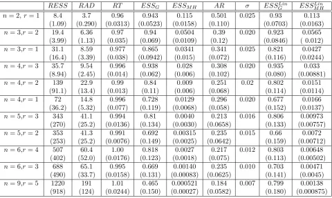
as RAD =ADG/ADM H. We compare the algorithms for a range of values ofn and r. For each pair (n, r)
we generate 100 fictitious samples and run both algorithms for each of these samples. The average values of
RESS, RAD, ESSG, ESSM H, ESSGLin, ESSM HLin and their standard deviations together with other summaries
are reported in Table 1 for ρ= 0.3 and in Table 2 for ρ= 0.98. From Table 1, when n= 2 and r = 1, our
algorithm is almost as efficient as independent sampling (ESS= 0.95), whereas the MH algorithm is about 8.4
times less efficient (in terms of ESS). Moreover, the relative gains increase as n gets larger. Forn = 6 and
r= 3 our algorithm is on average 666 times more efficient, and forn= 9 andr= 5 it is about 1270 times more
efficient. A similar pattern is observed when efficiency measures are calculated for the parameters of the linear
normalization (ESSLin
G and ESSM HLin) and substantial improvements are also observed in terms of the average
update distance. Furthermore, our algorithm computes 15000 iterations slightly more quickly than the M H
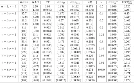
algorithm (RT), suggesting that the gains adjusted for computation time are even higher. Table 2 shows that
when ρ = 0.98, which implies that α is close to zero and thus β is weakly identified, the results are similar.
Thus, weak identification does not seem to have a significant impact on the speed of convergence. Recall that
β is restricted to be semi-orthogonal, and note that the space of semi-orthogonal matrices has a finite measure.
Thus, the posterior forβ conditional onα= 0 is proper, and thus no problems of local non-identification arise.
From the computational side, a draw ofα(∗)(orB(s)) close to zero could potentially cause numerical problems
at the time of calculating the inverse of (α′
α) (or the inverse of (B′
B)). We did not find this problem in our
calculations, but note thatAandβcan be calculated without using inverses. In particular, ifU :n×r,S:r×r, and V : n×r form the singular value decomposition of α=U SV′
, then A can be calculated as6 A =U V′
.
Similarly, ifU, S, V form instead the singular value decomposition ofB, thenβ can be calculated asβ =U V′
.
5.2
Collapsed Gibbs versus parameter augmented Gibbs
We use the same prior for Σ, but use the proper prior for (α, β) described in Sections 3 and 4, withτ = 1,G=In
andnν = 2, sν= 1. This prior allows for a large prior variance forα, sincea priori P r(ν >49.75) = 0.01. Table
3 shows efficiency measures for these two algorithms whenρ= 0.8. The collapsed Gibbs is slightly more efficient
for some values of (n,r) according to some indicators, but overall it seems that the parameter augmented Gibbs
is almost as efficient in practice as the collapsed Gibbs sampler. In our implementation, however, the collapsed
6Note that becauseUandV are semi-orthogonal,α= (U V′)(V SV′), whereU V′is semi-orthogonal and (V SV′) is a symmetric positive definite matrix. From the uniqueness of the polar decomposition (e.g. Cadet (1996)), it follows that A = U V′ and
Gibbs sampler needed slightly less computing time to do the same number of iterations.
When ρ is close to one, there is little information about the cointegrating space in the data. Thus, the
algorithms will explore large regions of the parameter space. In order to illustrate this, we simulate 500 artificial
datasets as described above for (n= 2,r= 1) and several values ofρ. In each of them we calculate the maximum
distance (MD) between the draws and the posterior mean of p=sp(β), where the posterior mean of the space
is defined as in Villani (2006). Note that in the case (n= 2,r= 1) the distance measure is bounded between 0
and 1 (Larsson and Villani (2001)). Table 4 shows that whenρ= 0.3M D is small on average, but whenρ= 1
M D is always equal to one, which implies that the algorithm visits all regions of the parameter space.
As an aside, which is unrelated to computational properties, Table 4 also calculates the frequentist coverage
of 95% and 99% credible intervals. That is, it calculates the proportion of times that a 95% (or 99%) credible
interval contains the true value of the cointegrating space. Note that Bayesian credible intervals are designed
to have correct Bayesian coverage (e.g. Raftery and Zheng (2003)), but they often also have correct frequentist
coverage (Bernardo and Smith (1994, p. 359)). We construct credible intervals as the set of spaces whose
distance to the mean is smaller than a given distance x. For a 95% credible interval, the distance x is the
95% percentile of the distances between the draws and the posterior mean ofp. Table 4 suggests that Bayesian
credible intervals have correct frequentist coverage when ρ = 0.3 and ρ = 0.9. However, when ρ = 1 the
frequentist coverage of a 95% (or 99%) credible interval is smaller than 95% (or 99%).
6
Conclusions
We have developed efficient and simple algorithms for cointegration models in a framework that allows putting
a prior, possibly Uniform, directly on the cointegrating space. This approach avoids the problem that arises
when putting a commonly used and tractable prior on the linearly normalized cointegrating vectors (Strachan
and van Dijk (2004)), which implies an awkward prior for the cointegrating space. In addition, the approach
avoids the problem of non-convergence in the Gibbs sampler caused by local non-identification (Kleibergen and
van Dijk (1998)).
References
Abadir, K. and Magnus, J., 2005, Matrix Algebra. Cambridge: Cambridge University Press.
Bauwens, L. and Lubrano, M., 1996, Identification restrictions and posterior densities in cointegrated Gaussian
Bauwens, L., Lubrano, M. and Richard, J.-F., 1999,Bayesian Inference in Dynamic Econometric Models. Oxford:
Oxford University Press.
Bernardo, J.M. and Smith, A.F.M. 1994. Bayesian Theory, Wiley, Chichester.
Brooks, S., 1999, Bayesian analysis of animal abundance data via MCMC, in Bayesian Statistics 6 (ed. J.M.
Bernardo, J.O. Berger, A.P. Dawid, A.F.M. Smith). Oxford: Clarendon Press.
Cadet, A., 1996, Polar coordinates in theRnp; Application to the computation of the Wishart and Beta Laws,
Sankhya: The Indian Journal of Statistics 58, 101-114.
Chib, S. and Greenberg, E., 1995, Understanding the Metropolis-Hastings algorithm,The American Statistician
49, 327-335.
Chikuse, Y., 1990, The matrix angular central Gaussian distribution, Journal of Multivariate Analysis 33,
265-274.
Chikuse, Y., 2003, Statistics on special manifolds, volume 174 of Lecture Notes in Statistics, Springer-Verlag,
New York.
DeJong, D., 1992, Co-integration and trend-stationarity in macroeconomic time series,”Journal of Econometrics
52, 347-370.
Dorfman, J., 1994, A numerical Bayesian test for cointegration of AR processes, Journal of Econometrics 66,
289-324.
Geweke, J., 1996, Bayesian reduced rank regression in econometrics, Journal of Econometrics 75, 121-146.
Geyer, C.J., 1992, Practical Markov chain Monte Carlo,Statistical Science 7, 473-511.
Holmes, C.C. and Held, K., 2004, Bayesian auxiliary variable models for binary and polychotomous regression,
forthcoming inBayesian Analysis.
Johansen, S., 1995,Likelihood-Based Inference in Cointegrated Vector Autoregressive Models. Oxford: Oxford
Uni-versity Press.
Kleibergen, F. and Paap, R., 2002, Prior, posteriors and Bayes factors for a Bayesian analysis of cointegration,
Journal of Econometrics 111, 223-249.
Kleibergen, F. and van Dijk, H.K., 1994, On the shape of the likelihood/posterior in cointegration models,
Econometric Theory 10, 514-551.
Kleibergen, F. and van Dijk, H.K., 1998, Bayesian simultaneous equations analysis using reduced rank
struc-tures,Econometric Theory 14, 701-743.
Koop, G., 1994, An objective Bayesian analysis of common stochastic trends in international stock prices and
Koop, G., Strachan, R., van Dijk, H.K. and Villani, M., 2005, Bayesian approaches to cointegration. To appear
in T.C. Mills and K. Patterson (eds.). Palgrave Handbook of Theoretical Econometrics, manuscript available
at http://www.le.ac.uk/economics/research/RePEc/lec/leecon/dp04-27.pdf.
Larsson, R. and Villani, M., 2001, A distance measure between cointegration spaces, Economics Letters 70,
21-27.
Liu, J.S., 1994, The collapsed Gibbs sampler with applications to a gene regulation problem, Journal of the
American Statistical Association 89, 958-966.
Liu, J.S., Wong, W.H., and Kong, A., 1994, Covariance structure of the Gibbs sampler with applications to
comparisons of estimators and augmentation schemes,Biometrika 81, 27-40.
Madan, D.B. and Seneta, E., 1990, The Variance-Gamma (V.G) Model for Share Market Returns, Journal of
Business 63, 511-524.
Muirhead, R. J. (2005) Aspects of Multivariate Statistical Theory,New Jersey: Wiley.
Raftery, A. E., Zheng, Y. 2003. Discussion: Performance of Bayesian Model Averaging. Journal of the American
Statistical Association, 98, 931-938.
Strachan, R., 2003, Valid Bayesian estimation of the cointegrating error correction model, Journal of Business
and Economic Statistics 21, 185-195.
Strachan, R. and Inder, B., 2004, Bayesian analysis of the error correction model,Journal of Econometrics 123,
307-325.
Strachan, R. and van Dijk, H., 2004, Valuing structure, model uncertainty and model averaging in vector
autoregressive processes, Econometric Institute Report EI 2004-23, Erasmus University Rotterdam.
Villani, M., 2005, Bayesian reference analysis of cointegration,Econometric Theory 21, 326-357.
RESS RAD RT ESSG ESSM H AR σ ESSGLin ESSM HLin
n= 2,r= 1 8.4 3.7 0.96 0.943 0.115 0.501 0.025 0.93 0.113
(1.09) (0.290) (0.0313) (0.0523) (0.0158) (0.110) (0.0703) (0.0163)
n= 3,r= 2 19.4 6.36 0.97 0.94 0.0504 0.39 0.020 0.923 0.0565
(3.99) (1.13) (0.035) (0.069) (0.0109) (0.12) (0.0846) ( 0.012)
n= 3,r= 1 31.1 8.59 0.977 0.865 0.0341 0.341 0.025 0.821 0.0427
(16.4) (3.39) (0.038) (0.0942) (0.015) (0.072) (0.116) (0.0244)
n= 4,r= 3 35.7 9.54 0.996 0.938 0.028 0.308 0.020 0.935 0.033
(8.94) (2.45) (0.014) (0.062) (0.006) (0.102) (0.080) (0.00881)
n= 4,r= 2 139 22.9 0.99 0.84 0.009 0.251 0.02 0.802 0.0151
(91.1) (13.4) (0.013) (0.11) (0.006) (0.068) (0.114) (0.0114)
n= 4,r= 1 72 14.8 0.996 0.728 0.0129 0.296 0.020 0.677 0.0166
(36.2) (5.32) (0.077) (0.119) (0.0068) (0.058) (0.152) (0.0137)
n= 5,r= 3 343 41.1 0.994 0.81 0.0040 0.213 0.016 0.806 0.00973
(270) (25.2) (0.0136) (0.134) (0.0030) (0.0658) (0.133) (0.00757)
n= 5,r= 2 353 41.3 0.991 0.692 0.00315 0.235 0.015 0.66 0.0072
(253) (25.2) (0.0076) (0.149) (0.0025) (0.0642) (0.159) (0.00712)
n= 6,r= 4 507 60.4 1.00 0.818 0.0027 0.217 0.012 0.803 0.00648
(402) (52.0) (0.0176) (0.123) (0.0018) (0.075) (0.113) (0.00502)
n= 6,r= 3 688 65.1 0.995 0.669 0.00140 0.235 0.010 0.703 0.00471
(490) (33.7) (0.0158) (0.131) (0.00083) (0.0625) (0.141) (0.0045)
n= 9,r= 5 1220 191 1.01 0.465 0.000521 0.184 0.007 0.799 0.00138
[image:16.595.74.555.215.502.2](918) (124) (0.0244) (0.150) (0.00027) (0.0582) (0.180) (0.000875)
Table 1: Performance measures of our algorithm and the M H algorithm, averaged over 100 fictitious samples for each value of (n, r) (ρ= 0.3). The columns RESS, RAD, ESSG, ESSM H, ESSGLin, ESSM HLin are defined in
RESS RAD RT ESSG ESSM H AR σ ESSLinG ESSM HLin
n= 2,r= 1 7.63 3.70 0.95 0.838 0.122 0.475 0.5 0.996 0.725
(2.84) (1.08) (0.055) (0.127) (0.0367) (0.179) (0.0109) (0.290)
n= 3,r= 2 35.7 9.64 0.98 0.876 0.0316 0.288 0.4 0.999 0.45
(17.9) (4.29) (0.0293) (0.0894) (0.0176) (0.105) (0.0108) (0.235)
n= 3,r= 1 21.2 9.15 0.963 0.57 0.035 0.251 0.5 0.988 0.402
(11.9) (4.60) (0.0872) (0.162) (0.0228) (0.12) (0.0429) (0.257)
n= 4,r= 3 114 18 0.992 0.916 0.0117 0.231 0.3 0.999 0.350
(100) (8.58) (0.013) (0.06) (0.007) (0.0837) (0.0105) (0.232)
n= 4,r= 2 152 31.1 0.992 0.706 0.0083 0.196 0.22 0.999 0.229
(133) (23.7) (0.016) (0.13) (0.0062) (0.0810) (0.0226) (0.188)
n= 4,r= 1 53.4 16.8 0.971 0.471 0.0112 0.202 0.3 0.978 0.260
(33.3) (8.14) (0.0538) (0.152) (0.0060) (0.0752) (0.0726) (0.223)
n= 5,r= 3 345 43.7 0.994 0.746 0.00312 0.219 0.10 0.998 0.227
(222) (25.3) (0.0168) (0.102) (0.00207) (0.0744) (0.0269) (0.195)
n= 5,r= 2 267 41.2 0.987 0.576 0.0035 0.226 0.09 0.999 0.195
(240) (29.7) (0.0279) (0.118) (0.0023) (0.081) (0.0123) (0.154)
n= 6,r= 4 636 50.3 0.996 0.815 0.0021 0.300 0.04 0.999 0.316
(768) (28.2) (0.034) (0.086) (0.0014) (0.0847) (0.0079) (0.23)
n= 6,r= 3 512 56.9 0.998 0.652 0.0019 0.274 0.040 0.999 0.272
(414) (38.4) (0.015) (0.104) (0.0011) (0.0811) (0.0067) (0.221)
n= 9,r= 5 1300 150 1.00 0.659 0.00067 0.225 0.040 0.999 0.178
[image:17.595.74.541.84.371.2](784) (86.8) (0.0082) (0.0712) (0.00038) (0.0603) (0.0063) (0.172)
Table 2: Performance measures whenρ= 0.98. Labels defined in Table 1.
ESSG ESSP AG RT ESSGLin ESSP AGLin
n= 3,r= 2 0.752 0.424 0.638 0.989 0.993
(0.133) (0.072) (0.018) (0.036) (0.057)
n= 4,r= 2 0.477 0.316 0.624 0.991 1.008
(0.136) (0.088) (0.022) (0.038) (0.108)
n= 6,r= 4 0.573 0.538 0.606 0.999 0.999
(0.092) (0.091) (0.006) (0.005) (0.006)
n= 9,r= 5 0.575 0.595 0.648 0.996 0.999
[image:17.595.70.388.406.520.2](0.072) (0.068) (0.006) (0.037) (0.005)
Table 3: Performance measures averaged over 100 samples: collapsed Gibbs versus parameter augmented Gibbs (ρ= 0.8). ESSG and ESSGLin refer to the collapsed Gibbs of Section 3 and ESSP AG and ESSP AGLin refer to
the parameter augmented Gibbs of Section 4. RT is the ratio of computation time of collapsed Gibbs over the other Gibbs. Standard deviations are in parentheses.
M DG M DP AG COVG95 COVP AG95 COVG99 COVP AG99
ρ= 0.3 0.124 0.141 0.94 0. 954 0.988 0.988
ρ= 0.9 0.987 0.998 0.932 0.962 0.986 0.994
ρ= 1 1.000 1.000 0.594 0.694 0.852 0.944
Appendix for Proofs:
Proof of Proposition 1. The prior for(α, β)is proportional to:
β′P
1/τβ
−n/2
β′P 1/τβ
n/2
exp
−1
2tr ν
−1
β′P
1/τβα′(G)−1α
whereβ′P 1/τβ
−n/2
is part of the prior forβandβ′P 1/τβ
n/2
is part of the conditional prior ofαgivenβ. Recall
that α=Aκ, where κ is a symmetric positive definite matrix, and let K=κ2. Using Lemma 2.1 in Chikuse
(1990), this prior for(α, β) implies that the prior for(A, K, β) is proportional to:
exp
−1
2tr ν
−1β′P
1/τβκA′(G)−1Aκ
|K|
n−r−1
2
where|K|−n−r−1
2 is the Jacobian of the transformation (Muirhead 2005, Theorem 2.1.14). Using the properties
of the trace of a matrix, and noting thatB=βκ, this expression can be written as:
exp
−1
2tr ν
−1
A′(G)−1
AB′P 1/τB
|K|
n−r−1
2
Therefore, taking into account that the Jacobian from(A, K, β) to (A, B) is |K|−n−r2−1, the prior for (A, B) is proportional to:
exp
−1
2tr ν
−1A′(G)−1AB′P 1/τB
Since(Pτ)−1 =P1/τ, this shows that the prior ofB givenAis given by (11). If we integrate with respect toB,
we get the prior forA:
ν A′(G)−1
A−1⊗Pτ
1/2
=|Pτ|r/2
ν A′(G)−1
A−1
n/2
∝A′(G)−1A−n/2
which is proportional to aM ACG(G).
Proof of Proposition 2. From Theorem 2.2 in Chikuse (1990), ϕ|(ν, τ) follows a MACG(Pτ). To prove that
D2|(ϕ, ν, τ)follows a Wishart, note that the joint prior of (ϕ,e αe)|(ν, τ) is proportional to:
π(ϕ,e αe|ν, τ)∝exp
−1
2tr sϕe
′P−1
τ ϕe
exp
−1
2tr ν
−1 e
α′G−1 e
α
(13)
Note thatϕe=ϕD and thattr sϕe′P−1
τ ϕe
=tr sϕeϕe′P−1
τ
=tr sD2ϕ′P−1
τ ϕ
. Recall also that the Jacobian from
(ϕ,e αe) to (ϕ, D2,eα) is D2(s−r−1)/2 (Muirhead 2005, Theorem 2.1.14). Thus, (13) implies thatπ(ϕ, D2,αe|ν, τ) is proportional to:
π(ϕ, D2,αe|ν, τ)∝D2(s−r−1)/2exp
−1
2tr sD
2
ϕ′P−1
τ ϕ
exp
−1
2tr ν
−1 e
α′G−1 e
α
which shows that D2|(ϕ, ν, τ) is aWr(s, sϕ′Pτ−1ϕ
−1
). To calculate the first moments ofα, note that α=αDe ,
and thatE(αe|D) = 0. Thus, E(αDe |D) =E(α|D) = 0. By the law of iterated expectations,E(α) = 0. Next from
vec(α) =vec(αDe ) = (D′⊗I
n)vec(αe)and var(vec(αe)|D, ϕ, τ, ν) =ν(Ir⊗G), it follows that var(vec(α)|D, ϕ, τ, ν) =
ν(D2⊗G). By the law of iterated expectations, and the properties of the Wishart distribution,var(vec(α)|ϕ, τ, ν) =
(ν(E(D2|ϕ, τ, ν)⊗G)) =ν( ϕ′P−1
τ ϕ
−1 ⊗G)
Proof of Proposition 3. The proof consists in showing that the integral of the posterior with respect toΣ is
never larger than a constant times the prior. Hence, a proper prior results in a proper posterior. Let us first
consider the case in whichGis a known matrix. Letπ(α,e ϕe)be the prior of(α,e ϕe). The integral of the posterior
with respect toΣis:
π(α,e ϕe|Data)∝hy−Xeϕeαe′i′hy−Xe e
ϕαe′i
−T /2
π(α,e ϕe)
which can be written as:
ϕeαe′−Πb′Ω−1 e
ϕαe′−Πb+y′y−Πb′Ω−1Πb
−T /2
π(α,e ϕe) (14)
where:
Ω = (Xe′Xe)−1
b
Π = ΩXe′y
Expression (14) is never greater than:
y′y−Πb′Ω−1Πb
−T /2π(α,e ϕe) (15)
Thus, ifπ(α,e ϕe)is proper then the posterior is proper. WhenG= Σthe integral of the posterior with respect to
Σis:
π(α,e ϕe|Data)∝hy−Xeϕeαe′i′hy−Xe e
ϕαe′i+ e α′ e α
−(T+r)/2
π(ϕe)
which, using the same reasoning as before, is never greater than:
y′y−Πb′Ω−1Π +b e
ααe′
−(T+r)/2π(ϕe) (16)
which is the product of a matricvariate Student Distribution (Bauwens et al. 1999, p. 307) withT degrees of
freedom times the prior ofϕe. Hence, the integral of (16) is finite, and thus the posterior is proper.
Appendix for other over-identifying restrictions
Consider the restriction (e.g. (Johansen 1995, p. 73))β= ( F1ϕ1 F2ϕ2) , whereF1andF2are known matrices.
We can partitionαconformably as: α= ( α1 α2) , so that
βα′=F
In a similar manner to Section 4, we introduce non-identified conformable squared matricesD1andD2as follows:
F1ϕ1α′1+F2ϕ2α′2 = F1ϕ1D1D1−1α′1+F2ϕ2D2D−12 α′2
= F1ϕe1αe′1+F2ϕe2αe′2
If Normal priors are chosen for(αe1,αe2,ϕe1,ϕe2)then the Gibbs sampling algorithm consists in sampling