arXiv:quant-ph/9903024 v1 5 Mar 1999
Creation of coherence in Bose-Einstein condensates by atom detection
Peter Horak and Stephen M. Barnett
Department of Physics and Applied Physics, University of Strathclyde, Glasgow G4 ONG, United Kingdom (June 28, 2006, submitted to Phys. Rev. A)
We investigate the creation of a relative phase between two Bose-Einstein condensates, initially in number states, by detection of atoms and show how the system approaches a co-herent state. Two very distinct time scales are found: one for the creation of the interference is of the order of the detection time for a few single atoms and another, for the preparation of coherent states, of the order of the detection time for a significant fraction of the total number of atoms. Approxi-mate analytic solutions are derived and compared with exact numerical results.
PACS number(s): 03.75.Fi, 05.30.Jp, 42.50.Ar
I. INTRODUCTION
The first experimental realisations of Bose-Einstein condensation in dilute atomic gases [1–3] have opened up a new field in atomic and quantum physics. Despite its apparent complexity, the condensate is well-described by a macroscopic wavefunction, or complex field, obeying a nonlinear wave equation (the Gross-Pitaevskii equation). The nature of this complex field and in particular its ap-parent phase has been the subject of some debate.
One specific topic which has been frequently investi-gated is the question of the coherence properties [4,5] of Bose-Einstein condensates as established in interference experiments [6,7]. The underlying question is whether the phase or, more precisely, the relative phase of two condensates is created by a spontaneously broken sym-metry [8] or by some other mechanisms [9]. It has been suggested [10] (and studied in detail by several authors [11–16]) that such a relative phase can be created by the detections of individual atoms in an interferometric setup, that is, where the origin of the detected atoms is intrinsically unknown. This process gives rise to a defi-nite (but unpredictible) relative phase of two condensates even if the initial states of the condensates are of unde-fined phase, as for initial number states [10,11,13], initial Poissonian states [12,14], or initial thermal states [14], by entangling the states of the two condensates.
In this work we will study in detail the creation of coherence between two condensates which initially have well defined occupation numbers, not only in the limit where the number of atoms detected is small compared to the total number of atoms but also in the long time limit. We concentrate thereby on two manifestations of coherence: the creation of interference fringes and the evolution of the compound two-condensate system to-wards a kind of coherent state. We start with an
ideal-ized model (Secs. III-IV) and later introduce more realis-tic features including atomic collisions (Sec. V). We use exact numerical simulations combined with approximate analytical solutions to determine the time evolution of our system. We show that these two measures of coher-ence are created on very different time scales. The rela-tive phase associated with the appearance of interference fringes develops in a time of order 1/(N γ), where N is the total initial number of atoms in the two condensates andγ is the rate at which atoms leak out of the conden-sates and are detected. The approach towards coherent states, in contrast, takes a larger time of order 1/γ. These two timescales correspond to timescales recently identi-fied for the interaction of a Bose-Einstein condensate or other bosonic system with its environment [17]. In this case, a well-specified atom number will change on the timescale 1/(N γ) but any coherence present decays on a timescale 1/γ.
II. MODEL
Let us first introduce the model system which we use to investigate the coherence properties in Bose-Einstein condensation [10–16]. We consider two independent non-interacting single-mode Bose-Einstein condensates with creation (annihilation) operators a† (a) and b† (b),
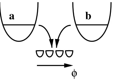
re-spectively. Atoms are leaking out of the condensates and are detected individually and spatially resolved. The same detectors simultaneously monitor decays from both condensates, that is, atoms coming from different con-densates are allowed to interfere, see Fig. 1. Thus, the detections are described by the annihilation operators
a(φ) =√1
2 a+be
−iφ
(1)
whereφ∈[−π, π] is related to the position of the detector xbyφ =px/¯h where pis the momentum of the atoms leaking out of the condensates.
Assume now that the system can be described at a cer-tain timetby a wave function|ψi. Then the probability of detecting the next atom at positionφis given by
P(φ) =N hψ|a(φ)†a(φ)|ψi (2)
where the normalisation constantN is chosen such that
Z π
−π
dφ P(φ) = 1. (3)
P(φ) = 1
2π[1 +βccos(φ−θ)] (4)
where
βc=
2|hψ|a†b|ψi|
hψ|a†a+b†b|ψi (5)
is the visibility of the interference fringes conditioned on the quantum state |ψi, and θ gives the most likely po-sition of detection of the next atom. It should be em-phasized that this visibility is not the one obtained by detecting a large number of atoms from the initial state |ψi, but the one obtained by preparing this state|ψivery often and measuring asingleatom in each run. This dif-ference is important since every detection changes the state of the system and thus changes the conditional vis-ibilityβc.
a
b
[image:2.612.89.271.258.387.2]φ
FIG. 1. Schematic representation of the interfering Bose-Einstein condensates.
This system has already been investigated by several authors [10–16] in order to show that the detection of atoms breaks the underlying symmetry of the system and thus creates interference fringes. This is true even if the initial state of the system does not exhibit any prefered phase so that βc = 0. It is the main purpose of our
work to quantify this creation of coherence between two initially uncorrelated Bose-Einstein condensates.
III. CREATING INTERFERENCE FROM INITIAL NUMBER STATES
In this section we will discuss the creation of interfer-ence fringes as a consequinterfer-ence of consecutive detections of atoms when the two condensates are initially in number states. The full system is given initially by the quantum state
|ψ0i=|n1, n2i. (6)
After the detection ofkatoms at positionsφ1,φ2, ...,φk
the (unnormalized) state of the system is then
|ψki= (a+beiφk). . .(a+beiφ1)|ψ0i. (7)
The conditional probability of detecting the (k+ 1)th atom atφk+1 then reads
P(φk+1|φk, ..., φ1) =
= 1 2π
hψk|(a†+b†e−iφk+1)(a+beiφk+1)|ψki
hψk|a†a+b†b|ψki
= 1 2π
hψk+1|ψk+1i
(N−k)hψk|ψki (8)
where N = n1+n2. Thus, the probability for the
se-quence of detectionsφ1,φ2, ...,φk is
P(φk, ..., φ1) =P(φ1)P(φ2|φ1)...=
= 1
(2π)k
hψk|ψki
N(N−1)...(N−k+ 1). (9)
The conditional visibilityβ (we will writeβinstead ofβc
in this section in order to simplify the notation) for the state afterk detections is
β= 2|hψk|a
†b
|ψki|
hψk|a†a+b†b|ψki
= 2|hψk|a
†b
|ψki|
(N−k)hψk|ψki
. (10)
Thus the average visibility afterkdetections is
hβik=
Z
dφ1...dφk
2 (2π)k
(N−k−1)! N! |hψk|a
†b
|ψki|.
(11)
Note, however, that this mean conditional visibility is rather difficult to access experimentally since it involves the averaging overensembles of experiments where each ensemble consists of repeatedly preparing the quantum state of the system by the same sequence of detections from the same initial number state and measuring the position of the next detection. Nevertheless, this proves to be a useful measure theoretically especially to describe the time scale on which interference is created as we will show later in this section.
For the first two detections, that is, k = 1, 2, the integral in Eq. (11) can be evaluated analytically with the results
hβi1=
2n1n2
(n1+n2)2−(n1+n2), (12)
hβi2=
4
πhβi1. (13)
Forn1=n2=N/2 we thus obtain [11,14]
hβi1=
1 2
1
1−1/N. (14)
For any initial number of atoms this is larger than 1/2, meaning that the first detection already increases the av-erage visibility from zero to more than half its maximum value of one.
following. Let us assume that the system starts in the quantum state |ψ0i = |n, ni (same number of atoms in
both condensates) and all detections occur at the same positionφ. Of course, this is a highly unlikely detection sequence, but this assumption gives surprisingly good ap-proximate results as we will see. Without loss of gener-ality we may assumeφ= 0. Thus
|ψki= (a+b)k|ψ0i. (15)
From this we obtain the norm of the state as
hψk|ψki= k
X
m=0
k m
2
hn, n|(a†)mam(b†)k−mbk−m|n, ni
= n!
2
(2n−k)!
k
X
m=0
k m
2
2n−k n−m
. (16)
We now approximate the binomial coefficients by Gaus-sians using
k m
≈2k
r
2 πke
−2
k(m−k/2)
2
(17)
and replace the sum overm by an integral from−∞to ∞which yields
hψk|ψki ≈
n!2
(2n−k)!2
2n+k2
π 1
p
k(4n−k). (18)
Analogously we obtain
hψk|a†b|ψki ≈ n!
2
(2n−k−1)!2
2n+k−12
π
e−1/k
p
k(4n−k−2)
(19)
and thus from Eq. (5) the final result
βk ≈e−1/k (20)
independent of n (to order 1/n). Hence, independent of the initial number of atoms in the condensates, it al-ways needs the same (and very small) number of detected atoms to create the interference. If the initial total num-ber of atoms is N and each atom decays with a rate γ out of the condensate, then the time to create the inter-ference pattern will thus be of the order of 1/(N γ).
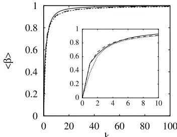
In Fig. 2 we compare the approximate result of Eq. (20) with the exact numerical solution of Eq. (10). The com-parison shows that the approximation is excellent fork as low as 2 (10% difference), 3 (5%) and 4 (3%) for n = 100, even if the approximation made in Eq. (17) only holds fork≫1. We also plot the numerical solution of Eq. (11), that is, the visibility averaged over all pos-sible outcomes with the appropriate probabilities which we obtained by Monte-Carlo simulations of the detection process. We see that the difference in the creation of in-terference fringes between the case where all atoms are
detected at the same place and the case where all pos-sible detection positions are allowed is relatively small. This is somewhat surprising given the great difference between the extremely peaked distribution of detection positions of our approximation compared with the ex-pected sinusoidal behavior [see Eq. (4)]. It is, however, a consequence of the fact that only a small number of detections determine the interference pattern for all sub-sequent detections.
0 0.2 0.4 0.6 0.8 1
0 20 40 60 80 100
<β>
k
0 0.2 0.4 0.6 0.8 1
[image:3.612.358.534.168.304.2]0 2 4 6 8 10
FIG. 2. Average conditional visibilityhβivs number of de-tected atomsk: exact numerical solution (solid curve), nu-merical solution if all atoms are detected at the same posi-tion (dashed curve), approximate analytical soluposi-tion (dotted curve). The initial state isn1=n2= 100.
So far we have restricted ourselves to the case of equal initial occupation numbers of the two condensates. In the case of unequal initial numbers the approximation assuming that all the detections occur at the same po-sition fails as it turns out that this changes the relative occupation of the two condensates (which is constant if the condensate decay rates are equal). An analytic ap-proximation can be found, however, assuming that the number of detected atomskis small compared to the to-tal number of atomsN. In this case the normalisation of the state afterkequal detections is
hψk|ψki=
=
k
X
m=0
k m
2
hn1, n2|(a†)mam(b†)k−mbk−m|n1, n2i
≈
k
X
m=0
k m
2
nm1nk2−m. (21)
The latter expression can be approximated by replacing the binomials with Gaussians and the sum by an integral as before. Applying the same procedure tohψk|a†b|ψki
one finally obtains the conditional visibility
βk ≈
2√n1n2
n1+n2
e−1/k (22)
Three features are worth mentioning here. First, the evolution of the visibility as a function of the number of detected atoms is the same as in the case of equal initial atom numbers. Hence, also in this case only a few detec-tions are required to establish the interference pattern and hence the corresponding time scale is again given by 1/(N γ). Second, the maximum possible visibility is reduced to a value which depends on the ratio of the ini-tial occupation numbers of the two condensates. Third, this maximum visibility is exactly the same as for initial coherent states of the condensates with the same mean numbers of atoms.
0 0.2 0.4 0.6 0.8 1
0 10 20 30 40 50
<β>
[image:4.612.98.270.203.339.2]n2
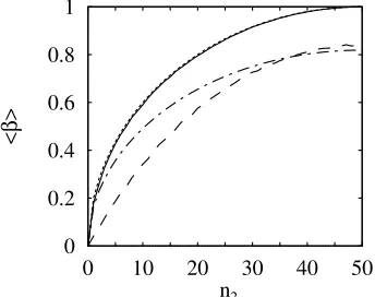
FIG. 3. Average conditional visibilityhβivs numbern2of
atoms initially in one of the condensates, the total number is n1+n2 = 100. Solid curve: exact numerical result after
99 detections, dashed: exact result after 5 detections, dotted: approximate analytic result after 99 detections, dash-dotted: approximate result after 5 detections.
In Fig. 3 we compare these results with the exact nu-merical solutions for arbitrary detection positions. We see that in the long-time limit, with nearly all of the atoms detected, the agreement is exact, thus the visibil-ity approaches the value found for coherent states of the same mean atom number. After a small number k of detections a more significant deviation from our approx-imate result is found, especially for significantly differing initial occupation numbersn1 andn2. However, we still
find that Eq. (22) predicts the correct order of magnitude for the time required to establish the interference.
IV. PREPARATION OF COHERENT STATES FROM INITIAL NUMBER STATES
In this section we will discuss how the system state approaches a coherent state in course of the sequence of detections. However, in order to simplify the discussion and the numerical simulations we will assume that the total number of atoms in the two condensates is exactly known at any time; the system is initially in a number state|n1, n2iwithn1atoms in condensateaandn2atoms
in condensate b and the number k of detected atoms is known at any time. Thus the system will never approach
a harmonic oscillator coherent state, that is, an eigen-state to the annihilation operatorsa and b, since these are superposition states of different total atom numbers. Instead it will be shown that the system approaches a state which can be described as the restriction of a co-herent state to the subset of states with a fixed total number of atoms. Hereafter we will refer to these states as “atomic coherent states” as they are a representation of the atomic coherent states [18]. We can define these states to be
|µ, νiN =
1 √
N! a
†µ+b†νN
|0,0i (23)
where µand ν obey the relation |µ|2+
|ν|2 = 1. Some
properties of these atomic coherent states and their rela-tion to the coherent states are discussed in Appendix A. The specific case of these states withµ=eiφ/√2 and
ν =e−iφ/√2 has also been refered to as “phase states”
[13,16],
|φiN =
1 √
2NN! a
†eiφ+b†e−iφN
|0,0i (24)
since their conditional visibility isβc= 1.
The problem which we will consider in this section is the following. Assume the system is initially in the num-ber state|ψ0i=|n1, n2i. Thenk atoms are detected at
positions φ1, φ2, ..., φk and the resulting state |ψki is
analyzed. What is the probability of finding an atomic coherent state|µ, νiN−k, whereN =n1+n2? To answer
this we have to evaluate the probability function
P(µ, ν) = |hψk|µ, νiN−k|
2
hψk|ψki
, (25)
or equivalently
P(φ) = |hψk|φiN−k|
2
hψk|ψki
(26)
in the case ofn1=n2=N/2.
Let us consider first the case of equal initial atom num-bersn1=n2=n and assume without loss of generality
that the first atom is detected at positionφ1= 0 so that
|ψ1i= (a+b)|n, ni. We then find
P(φ) = 1 22n
2n n
(1 + cos 2φ)≈ √1
πn(1 + cos 2φ)
(27)
where for the last approximation we have again used Eq. (17). One can easily check by numerical simulation that this approximation is highly acurate even for just a few atoms in the condensates. Hence the overlap of the state after one detection with any phase state is very small of the order of 1/√n.
and will compare the results forP(φ) with numerical sim-ulations at the end. The state overlap afterkdetections is then
hψk|φi2n−k =
1
p
22n−k(2n−k)!
×hn, n|(a†+b†)k(a†eiφ+b†e−iφ)2n−k|0,0i
= p n!
22n−k(2n−k)!
×
k
X
p=0
k p
2n−k n−p
eiφ(k−2p) (28)
which, after applying the approximation of Eq. (17), be-comes
hψk|φi2n−k≈
1
p
22n−k(2n−k)!
n!22n
√πne−φ42 k(2n−k)
n . (29)
This, together with the normalization factor, Eq. (18), yields
P(φ)≈1 2
r
k(4n−k) n2 e
−φ2 2
k(2n−k)
n . (30)
In the limit of k ≪ n this result is consistent with the results presented in Refs. [12,13,15].
0 0.2 0.4 0.6 0.8 1
-1 -0.5 0 0.5 1
P( )
φ
φ
[image:5.612.364.530.226.363.2]k=10 k=100 k=190
FIG. 4. ProbabilityP(φ) of finding the phase state|φiafter katom detections from initial state|n1= 100, n2 = 100i. The
solid curves correspond to exact numerical solutions (averaged over 1000 Monte-Carlo simulations) and the dashed curves to the analytic approximation given in Eq. (30).
In Fig. 4 we compare this analytic approximation for the probability function P(φ) with the exact numerical solution obtained by Monte-Carlo simulations where all possible detection positions are taken into account. (On the scale of Fig. 4 the curves for the approximate solu-tion and the exact solusolu-tion if all atoms are detected at the same position coincide almost exactly.) After only a few detections (k= 10 in the figure) the probability function is already well approximated by a broad Gaussian with a relatively small maximum, so the overlap with any phase state is still small at this time. However, we note that
the maximum overlap islarger than predicted by the ap-proximate analytic solution, which was derived under the assumption that all atoms are detected at the same posi-tion. This may seem surprising but can be explained by the fact that such a highly peaked position distribution of the detected atoms is far from the one expected for a coherent state. After the detection of half of the atoms (k = 100) the maximum overlap with a phase state is already close to one and the width of the Gaussian has decreased significantly. For a larger number of detected atoms (k = 190) the maximum overlap still increases but the width of the probability function increases again which is due to the changing non-orthogonality of the phase states for changing number of atoms, see Eq. (A3).
0 0.2 0.4 0.6 0.8 1
0 0.2 0.4 0.6 0.8 1
max{P( )}
µ,ν
k/N
FIG. 5. Maximum of the probability function P(µ, ν) after k atom detections out of the N = n1 + n2
ini-tial atoms. The solid curves correspond to the initial state |ψ0i = |n1 = 100, n2 = 100i, the dashed curve to |ψ0i=|n1 = 200, n2= 50i, and the dotted curve is the
maxi-mum of the approximate analytic solution, Eq. (30). The first two cases are the results obtained from averaging over 2000 Monte-Carlo simulations.
In Fig. 5 we plot themaximumof the probability func-tionP(µ, ν) as a function of the fraction of the detected atoms. The approximate solution given by Eq. (30) is in-dependent of the total numberN =n1+n2of atoms
ini-tially in the two condensates and is a quarter of a circle as a function ofk/N. As already seen above, the approach to an atomic coherent state starting from a pure number state is in fact faster than given by the approximation. Here we also plotted the numerical result for an initial state with unequal atom numbers in the two condensates and we note that also in this case the approximation by Eq. (30) is a relatively good one.
[image:5.612.101.268.378.513.2]V. GENERALISATIONS OF THE MODEL
A. Imperfect detection
We will now generalize our results from the previous sections to the case of imperfect atom detection. Assum-ing that the detector efficiency isη < 1 we expect that afterkatoms have been lost from the condensates onlyηk out of these are detected in the interferometric setup and thus contribute to the build-up of coherence between the two condensates, whereas the remaining (1−η)k atoms are simple losses from either of the two condensates.
Hence, under the assumption that all detected atoms are found at the same position (as in the previous sec-tions) and the undetected atoms are coming with the same probability from either of the two condensates, the state afterk atoms have been lost from the condensates is approximately
|ψki= (a+b)ηkaξkbξk|n, ni
= n!
(n−ξk)!(a+b)
ηk
|n−ξk, n−ξki (31)
[whereξ= (1−η)/2] instead of the one given in Eq. (15). Thus, in our earlier results, Eqs. (20) and (30), we only have to substituten→n−ξkandk→ηkto obtain the approximate results for imperfect detector efficiency
βk ≈e−1/(ηk), (32)
P(φ)≈
s
1−
1−2n ηk −k+ηk
2
e−φ2ηk(2n−k)2n−k+ηk. (33)
As in the previous sections, comparison of these analytic approximations with exact numerical solutions shows ex-cellent agreement for the visibility β and an actually faster approach towards coherent states as predicted by this approximation forP(φ).
Eq. (32) shows that the only effect of imperfect de-tection on the creation of interference fringes is that the number of atoms detected per unit time is decreased and and thus it takes more time to detect the same number of atoms as for perfect detectors. The effect of losses of atoms from individual condensates does not seem to have any influence even if this changes the relative atom num-ber in the two condensates. However, since only a few atoms need to be detected in order to build up the in-terference, the fluctuations of the condensate occupation numbers remain very small compared to the total number of atoms and thus the maximum visibility is very close to the one for the unperturbed initial state.
The situation is more complicated for the approach of the system state towards an atomic coherent state (or a phase state) because, not only the number of detected atoms, but also the total number of atoms left in the system plays an important role, so thatP(φ) depends on k and n. The preparation of an atomic coherent state also occurs on a larger time scale than forη= 1 but the dependence onη is not simple.
B. Proper time evolution
Another possible generalisation of our model is to vestigate the system evolution as a function of time in-stead of the number of detected atoms. Given a constant decay rate of γ for individual atoms from the conden-sates the actual decay processes still occur in a proba-bilistic manner. Thus after a certain amount of time the number of atoms remaining in the system is uncertain. However, since the condensate decay follows an exponen-tial law themean number of remaining atoms is
hni(t) =N e−2γt (34)
and so the mean number of detected atoms is
hki(t) =N 1−e−2γt
. (35)
We can generalise the results of the previous sections to incorporate this time evolution by simply replacing the numberkof detected atoms in Eqs. (20) and (30) by its mean value according to Eq. (35).
Using this assumption we compared the exact numer-ical results for the cases of the system evolution versus number of detections and versus time. We found that the visibility is established slightly more slowly in the latter case. Let us consider, for example, the state of the sys-tem after such a time t that hki(t) = 1. At this time there is still a significant probability that no atom was detected which greatly decreases the average visibility. On the other hand there is a certain probability that two or three atoms were detected which increases the average visibility, but since the difference between β0 and β1 is
much larger than the difference betweenβ1 and β2 [see
Eqs. (12), (13)] the former term dominates and the aver-age visibility is smaller thanβ1. However, this difference
between the results for the two models decreases when more atoms are detected and, starting from 100 atoms in each of the condensates, after k = 10 detections the numerically found difference is already down to 1.7%. A similar agreement is also found for the maximum overlap of the system state with atomic coherent states in the two models. We may thus conclude that our approxi-mate analytic solutions also describe the time evolution of the system if one substitutesk→ hki(t).
C. Effect of collisions
So far we have assumed the idealized case of noninter-acting particles in the condensates, so that our system was completely analogous to a system of photons in two high-quality cavities from which the photons decay and interfere. All of our previous results apply to this case as well [19].
our results in this case in the following. To this end, the free time evolution of the system between two quantum jumps now has to be replaced by the time evolution due to the collisional Hamiltonian which in our simple model of two single-mode condensates is [11,16,22]
H=κ
(a†a)2+ (b†b)2
. (36)
The action of this Hamiltonian is to give different time dependent phases to the various number states of the quantum state of the system of, for example, an atomic coherent state. This dephasing gives rise to a time depen-dent “decay” of the coherence and therefore of the condi-tional visibilityβ. This decay of the coherence counter-acts the creation of coherence due to atom detections and thus prevents the system of reaching a state of maximum visibility.
0 0.2 0.4 0.6 0.8 1
0 0.1 0.2 0.3 0.4
β
[image:7.612.104.271.257.397.2]tκ
FIG. 6. Time evolution of the conditional visibility β for different quantum states including collisions of atoms in the condensates. The initial quantum state is a state after 50 detections from the number state |100,100i (solid line), the state after 50 equal detections (a+b)50
|100,100i (dashed), and a phase state|φiN=150(dotted), respectively.
First we study the evolution of various quantum states under the action of the Hamiltonian (36) without atomic decays. Let the system initially be in an atomic coherent state with equal mean atom numberNin the two conden-sates,|ψi=|µ, µiN. The time evolution of the visibility
β, given by Eq. (5) can then be evaluated analytically as
β(t) = [cos(2κt)]N−1≈e−2κ2t2(N−1) (37)
where the latter approximation holds for small timest≪ 1/κ. Note that the exact result of Eq. (37) predicts the well known [13,16,22,23] revivals of the visibility after times which are multiples ofπ/(2κ).
As noted, however, in the preceding sections, the atomic coherent states are in general not a good approxi-mation to the state of the system until a significant num-ber of atoms have been detected. A better approxima-tion is provided by considering the evoluapproxima-tion of the initial state|ψki= (a+b)k|n, ni. Using again the
approxima-tion of Eq. (17) we obtain for this case
β(t)≈e−1/kexp
−2κ2t2k(2n−k−1) 4n−k−2
. (38)
In the limit of k ≪ n, we thus find that β decays as exp(−κ2t2k) which is much slower than the decay for an
atomic coherent state (37). Fork→2nthe two expres-sions converge since the state|ψkiapproaches an atomic
coherent state in this case.
In Fig. 6 we compareβ(t) for an atomic coherent state, the state|ψki, and the numerical result for a state after
50 detections from an initial number state|100,100i(all of these contain a total number of 150 atoms). We see that in any case the collision-induced decay can be well described by a Gaussian. The decay obtained for the state with simulated detections is faster than the one of Eq. (38) which agrees with our finding of Sec. III that an atomic coherent state is approached faster with arbi-trary detections than if all detections occur at the same position.
We will now use these results to derive an approximate analytic expression for the visibilityβ afterkdetections including the effects of atomic collisions. Let us assume that at a given time t0 exactly k atoms have been
de-tected from an initial number state |n, ni and that the visibility is β = β0. Then the probability of detecting
the next atom at timet0+tis given by
P(t) = 2n0γe−2n0γt (39)
where n0 = 2n−k is the number of atoms left in the
system at time t0. Thus, if we write the decay of the
visibility as
β(t0+t) =β(t0)e−t
2/τ2
, (40)
where τ is given in Eq. (38), then the visibility at the time immediately before the next atom detection is on average given by
hβ(t0+t)i=
Z ∞
0
dt β(t0+t)P(t)
=β(t0)2n0γτ
√π
2 e
n2
0γ2τ2[1−Φ(n
0γτ)], (41)
where Φ denotes the error function. Let us now assume that the system is in steady state between the creation and the decay of β, that is, the following detection in-creases the visibility again to its value β(t0) at time t0.
Hence, writing
β(t0) =e−1/k0≈1− 1
k0 (42)
and using our previous result for the increase ofβ with the number of detections, Eq. (20), we obtain the follow-ing condition
1− 1 k0
hβ(t0+t)i= 1−
1 k0−1
with the solution
k0= 1 +p 1
1− hβ(t0+t)i
(44)
and thus the steady state visibility is
βst=
1
1 +p1− hβ(t0+t)i
. (45)
0.5 0.6 0.7 0.8 0.9 1
0 40 80 120 160 200
<β>
[image:8.612.64.293.61.308.2]k
FIG. 7. Visibility β vs number of detected atoms k from an initial number state |100,100i including atom collisions. Solid lines are exact results (averages of 1000 Monte-Carlo simulations), dashed lines are the corresponding analytic ap-proximations given by Eq. (45). The parameters are (from top to bottom)κ= 0.5γ,κ= 2γ, andκ= 5γ.
We compare this result with the results of Monte-Carlo simulations in Fig. 7 for different values ofκ. From this we note that the approximation yields values of β that are too large. This is especially true for small numbers k of detected atoms (k < n). This was to be expected since (i) the approximation was based on the assumption of a steady state whereas it takes a certain number of de-tections to reach this state in the simulations and (ii) in the discussion of Fig. 6 we have already seen that the ac-tual decay of the visibility occurs faster than predicted by Eq. (38) which in turn decreases the steady state value. On the other hand, the approximation yields values ofβ below the numerical results for values ofβ < 0.8 where we know that the increase of the visibility due to detec-tions is faster than given by Eq. (20).
Finally we will investigate the effects of atomic colli-sions in the condensates on the creation of atomic co-herent states. To this end we calculate the maximum overlap of the time evolved state
|ψk(t)i=e−iHt|ψki, (46)
where|ψkiis the state afterkequal detections from the
number state |n, nias used before, with the atomic co-herent states. Following the same steps as in Sec. IV one obtains
max{P(φ, t)}= q max{P(φ, t= 0)}
1 + [tκk(2n−k)/(2n)]2
(47)
where max{P(φ, t= 0)}is the maximum overlap at time t= 0 given by Eq. (30). Hence, fork≪nthis maximum overlap decays on a time scale of t ∼ 1/(κk) which is much faster than the time scale of the decay of the visi-bility wheret∼1/(κ√k), Eq. (38). This, together with the much longer time scale necessary to create a signifi-cant overlap with coherent states, shows that atomic col-lisions have a much larger effect onP(φ, t) than on the visibility. The time scales for the decay and the build-up of this state overlap also prevent the system from reach-ing a steady state and thus no analytic approximation analogous to Eq. (45) can be found. Hence we have to rely on numerical simulations in this case, see Fig. 8.
0 0.2 0.4 0.6 0.8 1
0 40 80 120 160 200
max{P( )}
µ,ν
k
FIG. 8. Maximum overlap max{P(µ, ν)}vs number of de-tected atomskfrom an initial number state|n1=n2= 100i
including atom collisions with collision rateκ = 0.1γ (solid line),κ= 0.5γ(dashed), andκ= 5γ(dotted). Each curve is obtained from averaging over 1000 Monte-Carlo simulations. We note that for small numbers of detected atoms the maximum overlap increases close to the case ofκ= 0. For largerk, corresponding to a broader distribution of the relative atom number between the two condensates, the dephasing due to the atom collisions starts to dominate and significantly reduces max{P(µ, ν)} even for small values ofκ. However, when most of the atoms have been detected (k →2n) the function approaches unity as all one-particle states and the final vacuum state are exact atomic coherent states.
VI. CONCLUSIONS
[image:8.612.362.534.214.350.2]coherence, which in this article we describe by the over-lap of the quantum state of the system with coherent states, is created by detecting a certain (large)fraction of the condensed atoms, so the time scale for this de-velop is given by t ∼1/γ. These results were obtained from approximate analytic solutions as well as from exact numerical simulations.
We have also investigated the effect of atomic collisions on these results. In this case the dephasing of the quan-tum state of the system due to the collisions counteracts the entangling effect of the atom detections. However, ac-cording to the widely different time scales a good visibil-ity of the interference fringes can be maintained whereas the atomic collisions effectively prevent the preparation of a coherent state even for relatively small collision rates.
ACKNOWLEDGMENTS
This work was supported by the United Kingdom En-gineering and Physical Sciences Research Council.
APPENDIX A: ATOMIC COHERENT STATES
The atomic coherent states [18] were defined in Eq. (23) to be
|µ, νiN =
1 √
N! a
†µ+b†νN
|0,0i, (A1)
where|µ|2+
|ν|2= 1. These are states with preciselyN
atoms shared between the two condensates and can be expressed as an entangled superposition of all product number states for which the total number isN:
|µ, νiN =νN N
X
n=0
N n
1/2µ
ν
n
|n, N−ni. (A2)
The number of atoms in one of the condensates, there-fore, has a binomial distribution. Different atomic coher-ent states to the same number of atomsN are in general not orthogonal to each other, but have a nonvanishing scalar product
Nhµ′, ν′|µ, νiN = (µµ′∗+νν′∗)N. (A3)
The atomic coherent states are related to the familiar two-mode coherent states|α, α′
iby
|α, α′i=e−(|α|2+|α′|2)/2
∞ X
N=0
r
(|α|2+|α′|2)N
N! |µ, νiN
(A4)
with
µ= p α
|α|2+|α′|2, (A5)
ν = α
′
p
|α|2+|α′|2. (A6)
Clearly, the restriction of a two-mode coherent state to the N particle subset of states is an atomic coherent state.
The atomic coherent states satisfy the following useful identities
a|µ, νiN =
√
N µ|µ, νiN−1, (A7)
b|µ, νiN =
√
N ν|µ, νiN−1. (A8)
From these it immediately follows that the expectation values ofaandbin an atomic coherent state are zero so that neither condensate exhibits a prefered phase. It is also clear that the mean number of atoms in the conden-satesaandbareN|µ|2andN
|ν|2, respectively, and that
the expectation value ofa†bisN µ∗ν. It follows that the
conditional visibility for an atomic coherent state is
βc= 2|µ||ν| (A9)
which assumes its maximum value of unity if and only if the two condensates have the same mean occupation number. Restricting considerations to equal mean occu-pation numbers leads to the phase states [13,16] defined in Eq. (24). Further properties of the atomic coherent states can be found in the literature [18].
[1] M. H. Anderson, J. R. Ensher, M. R. Matthews, C. E. Wieman, and E. A. Cornell, Science269, 198 (1995). [2] C. C. Bradley, C. A. Sackett, J. J. Tollett, and R. G.
Hulet, Phys. Rev. Lett.75, 1687 (1995).
[3] K. B. Davis, M.-O. Mewes, M. R. Andrews, N. J. van Druten, D. S. Durfee, D. M. Kurn, and W. Ketterle, Phys. Rev. Lett.75, 3969 (1995).
[4] E. A. Burt, R. W. Ghrist, C. J. Myatt, M. J. Holland, E. A. Cornell, and C. E. Wieman, Phys. Rev. Lett.79, 337 (1997).
[5] W. Ketterle and H.-J. Miesner, Phys. Rev. A 56, 3291 (1997).
[6] M. R. Andrews, C. G. Townsend, H.-J. Miesner, D. S. Durfee, D. M. Kurn, and W. Ketterle, Science275, 637 (1997).
[7] D. S. Hall, M. R. Matthews, C. E. Wieman, and E. A. Cornell, Phys. Rev. Lett.81, 1543 (1998).
[8] A. J. Leggett and F. Sols, Found. Phys.21, 353 (1991). [9] Y. Kagan and B. V. Svistunov, Phys. Rev. Lett.79, 3331
(1997).
[10] J. Javanainen and S. M. Yoo, Phys. Rev. Lett.76, 161 (1996).
[11] T. Wong, M. J. Collett, and D. F. Walls, Phys. Rev. A
[12] J. I. Cirac, C. W. Gardiner, M. Naraschewski, and P. Zoller, Phys. Rev. A54, R3714 (1996).
[13] Y. Castin and J. Dalibard, Phys. Rev. A55, 4330 (1997). [14] R. Graham, T. Wong, M. J. Collett, S. M. Tan, and D.
F. Walls, Phys. Rev. A57, 493 (1998).
[15] J. Ruostekoski, M. J. Collett, R. Graham, and D. F. Walls, Phys. Rev. A57, 511 (1998).
[16] A. Sinatra and Y. Castin, Eur. Phys. J. D4, 247 (1998). [17] S. M. Barnett, K. Burnett, and J. A. Vaccarro, J. Res.
Natl. Inst. Stand. Technol.101, 593 (1996).
[18] The atomic coherent states, also known as spin coherent states and angular momentum coherent states, are famil-iar in discussions of rotation. J. M. Radcliffe, J. Phys. A: Math. Gen.4, 313 (1971); F. T. Arecchi, E. Courtens, R. Gilmore, and H. Thomas, Phys. Rev. A6, 2211 (1972); A. Perelomov,Generalized Coherent States and their Ap-plications(Springer-Verlag, Berlin, 1986); S. M. Barnett and P. M. Radmore, Methods in Theoretical Quantum Optics(Oxford University Press, Oxford, 1997).
[19] K. Mølmer, J. Mod. Opt.44, 1937 (1997).
[20] M. Lewenstein and L. You, Phys. Rev. Lett. 77, 3489 (1996).
[21] J. Javanainen and M. Wilkens, Phys. Rev. Lett.78, 4675 (1997).
[22] M. J. Steel and D. F. Walls, Phys. Rev. A 56, 3832 (1997).