The Remaining Useful Life Estimation of Lithium-ion Batteries Based on the HKA -ML-ELM Algorithm

Int. J. Electrochem. Sci., 14 (2019) 7737 – 7757, doi: 10.20964/2019.08.44

International Journal of

ELECTROCHEMICAL

SCIENCE

The Remaining Useful Life Estimation of Lithium-ion Batteries

Based on the HKA -ML-ELM Algorithm

Yanying Ma1,2 _{, Dongxu Shen}1,2 _{, Lifeng Wu}1,2 _{, Yong Guan}1,2_{, Hong Zhu} 1,2,*

1 _{College of Information Engineering, Capital Normal University, Beijing 100048, China;}

2 _{Beijing Key Laboratory of Electronic System Reliability Technology, Capital Normal University,}

Beijing 100048, China

*_{E-mail: [email protected]}

Received: 8 April 2019 / Accepted: 4 June 2019 / Published: 30 June 2019

Lithium-ion batteries have become the core energy supply component for many electronic devices. An accurate prediction of the remaining useful life (RUL) of lithium-ion batteries is of great significance for battery management and ensuring the reliability of electronic devices. The extreme learning machine (ELM) algorithm has been applied to predict the RUL of lithium-ion batteries; however, there are some disadvantages in this method: (i). the single hidden layer structure of the ELM necessarily restricts its ability to capture effective features in high-dimensional data. (ii). the input weights and biases of the ELM are generated randomly, which affects its prediction accuracy. To overcome these problems, this paper proposes an HKA-ML-ELM method for predicting the RUL of lithium-ion batteries. First, a new multi-layer ELM (ML-ELM) network is constructed. By adding an input layer into the last individual ELM of the ML-ELM and implementing the random selection of these input nodes to partially connect with the hidden layer, the network has higher robustness and can effectively prevent over-fitting. Second, the heuristic Kalman algorithm (HKA) is used to optimize the input weights and biases parameters of the ML-ELM, which improves the prediction accuracy. Finally, RUL prediction experiments are carried out for battery packs with different rated capacities and different discharge currents. The experimental results verify the effectiveness of the proposed method. The comparisons with other algorithms show that the proposed method has better prediction accuracy.

Keywords: Lithium-ion battery, RUL prediction, ML-ELM, HKA

1. INTRODUCTION

bring about a catastrophe. It is crucial to predict the RUL of lithium-ion batteries in advance for system safety considerations [4,5].

the off-line data became available, it was able to predict the RUL earlier than the traditional methods and achieved good results. However, there are also some faults in artificial neural networks, especially the slow training speed, weak generalization ability and complex calculations.

dataset. Compared with the original ELM and HKA-ELM methods, the HKA-ML-ELM has higher prediction accuracy.

The rest of the article is organized as follows:

The second part briefly introduces the basic principles of the ELM, new ML-ELM structure, HKA and HKA-ML-ELM. The third part introduces the experiments. The fourth part presents the experimental results, compares this method with other methods and ends with a discussion. The fifth part is the conclusion and summary.

2. OUTLINE OF METHODS 2.1. Extreme Learning Machine

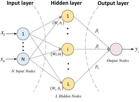
The ELM is a kind of machine learning algorithm based on the generalized single hidden layer feedforward neural network proposed by Huang, including the input layer, hidden layer and output layer. The ELM is classified and regressed by minimizing the predicted square loss and the norm of the output weight [30]. Its main characteristics are that the parameters of the hidden layer nodes can be set randomly or artificially without adjustment, and the learning process only needs to calculate the output weight. The high learning efficiency and strong generalization ability are the advantages of the ELM [31]. Its structure is shown in Fig. 1.

Figure 1. An ELM model

where x x1, 2,…,xn is the input matrix, W represents the connection weights between the input layer and the hidden layer, and b represents the biases of the hidden layer neurons. n represents the number of inputs, and L represents the number of hidden layer nodes:

11 1

1

n

L Ln L n

w w

W

w w _

 

 

=  

 

 

,

1

1

L L b b

b _

    =      

(1) 1

N

1

L i

1



n

x

1

x

(W b1,1)

(Wi bi, )

(W bL, L)

i 

L 

Output Nodes

L Hidden Nodes N Input Nodes

Input layer Hidden layer Output layer

j

Set the activation function of the hidden layer as h( ) , then the hidden layer output matrix of L hidden neurons can be expressed as:

( ) ( ) ( )

( ) ( ) ( )

( ) ( ) ( )

1 1 1 2 2 1 1

1 1 2 2 2 2 2

1 1 2 2

, , , , , ,

, , , , , ,

, , , , , ,

L L L L

N N L L N _{N L}

h w b X h w b X h w b X

h w b X h w b X h w b X

H

h w b X h w b X h w b X _

 

 

 

=  

 

 

 

(2)

j

y is the output, and its expression is:

(

)

1

, , , 1, 2, ,

L

i i i j j i

h w b x y j n

 =

= =



 1, 2,…,L are the connection weights between the hidden layer and the output layer. That is:

H=T (4)

The algorithmic process of the ELM is as follows:

Algorithm 1. The ELM algorithm

Step1. Determine the number of hidden layer nodes L, and randomly generate the connection weights W W1, 2, ,WL between the input layer and the hidden layer, as well as the biases b b1, 2, ,bL;

Step2. Determine the activation function h( ) and calculate the hidden layer output matrix H; Step3. The connection weights of the output layer can be calculated by solving the least square solution of the following equation:

min H T

  − (5)

The solution is:

 =H T+ (6) H+ is the generalized inverse of H.

2.2. A New ML-ELM Algorithm

The multilayer extreme learning machine (ML-ELM) was proposed by employing the ELM-based AEs (ELM-AEs), and its input layer is equal to the output layer. The ML-ELM integrates representation learning and classification into a single learning process, where the multiple layers of the ELM-AE are used for representation learning and the final layer of the ELM is used for classification. The ML-ELM learns the transformation from the hidden layer to the output layer, fixes all the parameters of each layer, and completes the iterative training. Therefore, the ML-ELM has a faster training speed, which can solve the time consumption problem of deep learning. Compared with the shallow structure of the ELM, the multi-layer structure of the ML-ELM enables it to capture more effective features in high-dimensional data. However, the ML-ELM directly uses the final data representation as the hidden layer to calculate the output weight, which does not guarantee the universal approximation capability of the ELM and leads to a high probability of over-fitting and low robustness [29,32].

improved, and over-fitting can be effectively prevented. The new constructed ML-ELM is shown in Fig. 2.

Figure 2. Architecture of the new ML-ELM

(a) The training mechanism randomly chooses input weights a1 and biases b1 for the input layer

of the AE, and then the transformation matrix _(1)

is obtained for representation learning in the ELM-AE.

(b) The learning process of the new input representation ( 2)

x is calculated by

(

)

g x   , where

g is an activation function.

(c) ( 2)

x is used as the input to the ELM-AE for the next representation learning step.

(d) The whole process of the ML-ELM from the input layer to the hidden layer and then to the output layer is shown. After the process of representation learning is completed, the final data representation final

x is selected as the input layer of an individual ELM. The random function is used to

generate several numbers, and the nodes corresponding to final

x are partially connected with the hidden

layer final

h , and then the output weight  is calculated. Here, c is the number of target classes.

2.3. Heuristic Kalman Algorithm

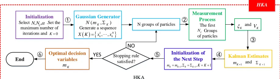
The HKA is an optimization algorithm that takes the optimization problem as a measurement process to obtain the optimal estimate [23]. The schematic diagram of the HKA [33] is shown in Fig. 3.

(1) 1 x (1) 2 x (1) d x (1) X Input (1) 1 x (1) 2 x (1) d x (1) X Output

( )1



( )1

h Hidden layer 1 (1) L h

( )1 1 h (1) 1 x (1) 2 x (1) d x (1) X Input (2) 1 x (2) 2 x 1 (2) L x (2) X New representation of input

( )1 (_ )T

1 (2) L x (2) 2 x 1 (2) L x (2) 2 x 1 1

(a , b ) (a , b )2 2

(afinal,bfinal) 

t 1 t 2 t c t

(a) (b) (c)

(d)

(2) 1 x

( )2 1 h 2 ( 2) L h (2) 1 x ( )2

h ( )2

 (i) 1 x (i) 2 x ( ) 1 i i L x ₋ ( )

(_i)T 1

final x 2 final x i final L x final h 1 final h j final L h (i) X final X ... ... ... ... ... ... ... ... ... ... ... ... (2) X(2) X (2) X Hidden layer Input Output (1) 1 x (1) 2 x (1) d x (1) X (1) 1 x (1) 2 x (1) d x (1) X

( )1  ( )1

h

1

(1)

L

h

( )1 1 h (2) 1 x (2) 2 x 1 (2) L x (2) X

( )1 (_ )T

1 (2) L x (2) 2 x 1 1

(a , b ) (a , b )2 2 ( )2

1 h 2 ( 2) L h (2) 1 x ( )2

h ( )2

 ... ... ... ... ... ... (2) X Output of ELM Hidden of ELM Input of ELM

Hidden layer of ML-ELM Input layer of

ML-ELM

Output layer of ML-ELM

ELM for Prediction

Figure 3. Schematic diagram of the HKA

The HKA is an iterative process. In the kth iteration of the HKA, x k( )is generated by the probability density function (pdf) pk( )x , and x k( ) is used as the input to the measurement process to generate the optimal value. In the Kalman estimation process, the optimal value is combined with pk( )x to generate a new pdfpk+1( )x as a reference for the next iteration [34]. The steps of the HKA are listed

below.

Algorithm 2. The HKA algorithm

Step1. Initialization. Set the HKA parameters: the number of particle groups, the number of best candidate groups, the deceleration coefficient, the number of iterations k = 0 and the maximum number of iterations.

Step2. Gaussian random generator (mk,k). A sequence of N vectors is generated according to the parameterized Gaussian distribution of the mean vector mk and variance-covariance matrix k: X(k)=





k k

x x , where i k

x is the ith vector generated in the kth iteration. Step3. Measurement. In the kth iteration, select





k k

x x  _{as the best candidate, and compute the}

optimal average value k of the best candidate and the variance value Vk after the selection.

1

1 N i

K K i x N    =

=



2 2

1, 1,K ,K n,K

1 1 1 ( ) , , ( ) T N N i i

K K n

i i

V x x

N      = =   =  − −   







Step4. Optimal estimation. In Kalman's framework, the estimators are expressed in the following forms:

mK+1=mK+LK (K−mK),

K+1=  +K K(WK− K) (9)

Among them,

1 K

( diag( ))

K K K

L =   + V − ,

2 ,k 1 2 ,K , 1 ₁ 1 1, 1

1, (w )

n i i K

n

i i K

i _{i n}

min v

n

min v max

n   = =    _{ }   _{  } _     =  _{  +}  _{ }   _{ }   





Select .Set the maximum number of iterations and

, ,

N N

0

K=

Gaussian Generator

Generate a sequence

( _K, _K)

N m 

( )  1 

, , N

k k

X K = x x

N groups of particles

Measurement Process The first Groups of particles N and K

 VK

Kalman Estimates

and

1

K

m + K+1

Initialization of the Next Step

1, 1, 1

K K K K

where vi K, represents the ith component of the variance vector Vk, and wi K, is the ith component

of the vector WK .

Step5. Initialize the next step. Set mK =mK+1 and  = K K+1.

Step6. The optimal value is obtained. If the termination rule is not satisfied, go back to Step2; otherwise, terminate the test and obtain the optimal value.

2.4. The HKA-ML-ELM

Since the connection weights and biases of the ML-ELM are generated randomly, and these two important parts will affect the prediction results, this paper uses the HKA to optimize the prediction framework of the ML-ELM. The HKA-ML-ELM includes two links: Link One is the process of the first n-1 layers of the ML-ELM, and Link Two is the process of the nth layer of the ML-ELM. The flow chart of the HKA-ML-ELM algorithm is shown in Fig. 4.

Figure 4. Architecture of the HKA-ML-ELM

Algorithm 3. The HKA-ML-ELM algorithm (a)Link One:

Step1. Initialize the parameter value of the ELM predictor and the total number of cycles n; Step2. Set the HKA parameters. Set the values of N N,  and , as well as the number of iterations k = 0 and the maximum number of cycles value;

Step3. Generate (m_K,_K). In each iteration, the normal distribution set is generated according to

the mean mK and standard deviation K of the Gaussian generator.

Step4. Random generator, According to the Gaussian distribution, N groups of X particles are randomly generated from (mK,K).

Step5. The generated particle X is used as the parameter of the ELM predictor, and the training set is brought into the ELM predictor for prediction.

N groups of particles

Measurement Process The first Groups

of particles N

Optimal decision variables

K

m

ELM Predictor

HKA-ML-ELM Predictor Start

Cost Function

Number of cycles satisfied?

NO Link

Two

YES

Train Set

Test Set

N groups of particles

Measurement Process The first Groups

of particles N

Optimal decision variables

K

m

ELM Predictor HKA-ML-ELM

Predictor

Cost Function

Selecting the Input nodes for partial connection and resetting Data set based on randomly generated numbers

Train Set Test Set

Start

Predictor Result

End

Link One Link Two

HKA HKA

Step6. The MSE of the predicted and real results is used as the cost function.

Step7. Select the optimal particle group. According to the order of the MSE values, for the first group N_ particles were selected from N groups as the candidate values.

Step8. Calculate the values of K and VK. The K value and VKvalue are calculated according to formulas (7) and (8) respectively.

Step9. The Kalman estimate. The values of mK+1 and K+1 are calculated according to formula (9).

Step10. Initialize the next update. Set mK=mK+1, = K K+1,k= +k 1.

Step11. Determine if the condition is met. If the number of iterations is reached, the iteration terminates, otherwise, it enters Step4.

Step12. Predict the test data. The optimum value mK is used as input weights and biases and is brought into the HKA-ML-ELM predictor with the test set for prediction.

Step13. Determine if the condition is met. If the maximum number of cycles is not reached, return to Step2. If the maximum number of cycles is reached, the cycle terminates, and Link Two is executed.

(b)Link Two:

Step1. Select the corresponding input nodes, based on the randomly generated number, to partially connect with the hidden layer.

Steps2-12. Same as Link One.

Step13. The predicted value is obtained.

3. EXPERIMENTS 3.1. Data Description

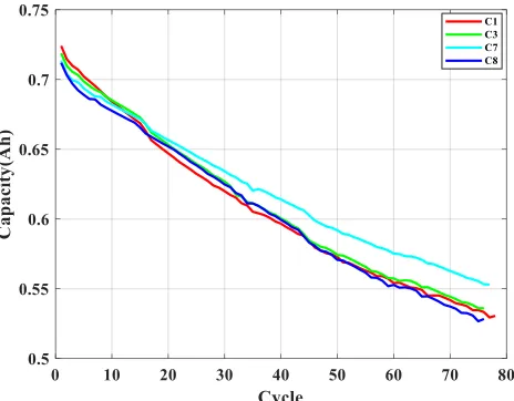
Figure 6. Change in the capacity of batteries C1, C3, C7 and C8

In this paper, there are two kinds of battery datasets.

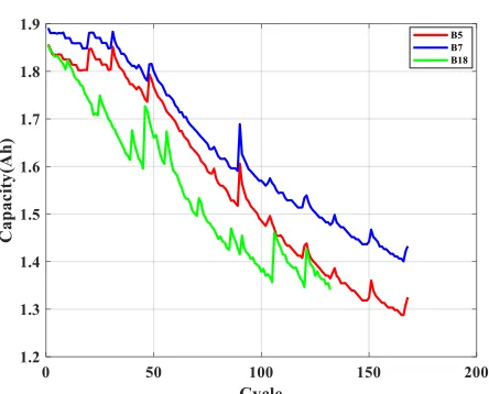
The first is from the NASA PCoE Research Center, which is available for public download on their website. Three groups of lithium-ion batteries (B5, B7 and B18) with a rated capacity of 2 Ah were used to charge, discharge and measure the resistance at 25 °C, and the monitoring data were recorded. The charge and discharge experiment method: charge in 1.5 A constant current mode until the battery voltage increases to 4.2 V, then continue to charge in constant voltage mode until the charging current drops to 20 mA. The voltages of B5, B7 and B18 are reduced to 2.7 V, 2.2 V and 2.5 V, respectively, at a constant current of 2 A. Repeated charging and discharging cycles can lead to accelerated battery ageing, while the impedance measurements can provide insight into the internal parameters of the battery as it ages. When the actual capacity of the battery was reduced to 70% of the rated capacity, that is, from 2Ah to 1.4Ah, the experiment was stopped [35]. The actual capacity of the B5, B7 and B18 batteries and the relationship between the charging and discharging cycles are shown in Fig. 5. Based on the HKA-ML-ELM algorithm, the RUL predictions are made for the three groups of data.

The second dataset is the Oxford University Battery Degradation dataset, which can be downloaded publicly on their website. Four groups of lithium-ion batteries (C1, C3, C7 and C8) with a rated capacity of 0.74 Ah were used in the experiment. The batteries were exposed to a constant-current-constant-voltage charging mode at 40 °C. Then, the driving cycle discharge profile was obtained from the Artemis urban profile. The characterization measurements were taken every 100 cycles until the end of the battery life, and monitoring data were recorded. The failure threshold was set at 75% of the rated capacity; that is, when the rated capacity decreased from 0.74 Ah to 0.555 Ah, the experiment stopped. The actual capacity of the C1, C3, C7 and C8 batteries and the relationship between the charging and discharging cycles are shown in Fig. 6. Based on the HKA-ML-ELM algorithm, the RUL predictions are made for the four groups of data.

3.2. Algorithmic Parameters and Evaluation Functions

Table 1. HKA-ML-ELM parameter values

B5 B7 B18 C1 C3 C7 C8

N 25 25 25 25 25 25 25

N_{ 5 5 5 5 5 5 5}

 0.4 0.4 0.4 0.4 0.4 0.4 0.4

L 1 1 1 1 1 1 1 Training set 83 83 65 38 37 37 37

Test set 82 82 64 37 36 37 36

In the above table, N and N are parameters of the HKA. L, Training set and Test set are

parameters of the ML-ELM.

This paper selects mean square error (MSE), correlation coefficient (R2_{) and absolute error (AE)}

as the evaluation functions to evaluate the prediction results.

4. RESULTS AND DISCUSSION

Two different datasets are selected for the experiments, namely, the NASA and Oxford University battery degradation datasets. The same dataset is tested with the ELM predictor, HKA-ELM predictor and HKA-ML-ELM predictor.

4.1. Results

The ELM algorithm and the HKA-ELM algorithm are selected as comparative experiments in this paper. The ELM parameters of the experiments are the same. Fig. 7, Fig. 8, Fig. 9, Fig. 10, Fig. 11, Fig. 12 and Fig. 13 correspond to the experimental results of B5, B7, B18, C1, C3, C7 and C8, respectively.

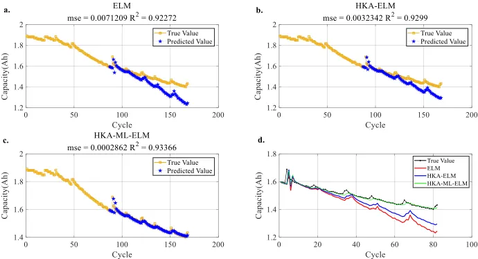
Fig. 7a, Fig. 7b and Fig. 7c represent the prediction results of the RUL of the B5 lithium-ion battery by using the ELM, HKA-ELM and HKA-ML-ELM algorithms, respectively. With the improvement of the algorithm, the predicted value is closer to the true value, and the predictive ability is continuously improved. Fig. 7d is a summary comparison of the predicted values and true value of all the methods used in this paper. Obviously, the HKA-ML-ELM algorithm has a higher prediction accuracy for the B5 lithium-ion battery.

Figure 8. Prediction of the RUL of B7

Fig. 8a, Fig. 8b and Fig. 8c represent the prediction results of the RUL of the B7 lithium-ion battery by using the ELM, HKA-ELM and HKA-ML-ELM algorithms, respectively. The predicted value of the ELM algorithm is the closest to the true value. According to Fig. 8d, the HKA-ML-ELM algorithm has higher prediction accuracy for the B7 lithium-ion battery.

Figure 9. Prediction of the RUL of B18

of the ELM algorithm is the closest to the true value. According to Fig. 9d, the HKA-ML-ELM algorithm has higher prediction accuracy for the B18 lithium-ion battery.

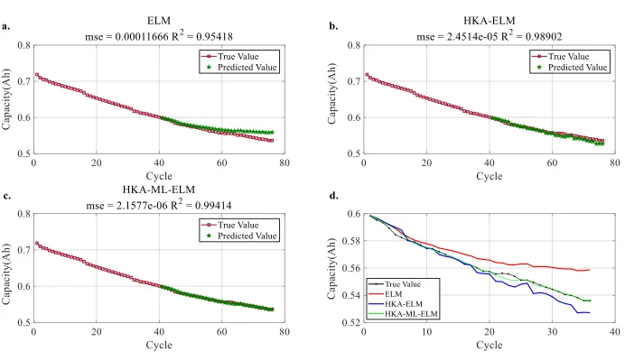
To further evaluate the predictive effect of the proposed method, the above experiments are carried out on lithium-batteries C1, C3, C7 and C8. Fig. 10a, Fig. 11a , Fig. 12a and Fig. 13a are the prediction results of the ELM algorithm. Fig. 10b, Fig. 11b, Fig. 12b and Fig. 13b are the prediction results of the HKA-ELM algorithm. Fig. 10c, Fig. 11c, Fig. 12c and Fig. 13c are the prediction results of the HKA-ML-ELM algorithm. Fig. 10d, Fig. 11d, Fig. 12d and Fig. 13d are the comparison summaries of the prediction results and true values of the three algorithms. Therefore, it can be seen that the HKA-ML-ELM algorithm has a better prediction effect. The experimental results are shown in the figures below.

Figure 10. Prediction of the RUL of C1

Figure 12. Prediction of the RUL of C7

Figure 13.Prediction of the RUL of C8 4.2. Discussion

The figures above show the predicted results of the seven experimental datasets. The HKA-ML-ELM has a higher predictive ability for the different datasets. Table 2 lists the evaluation results of the seven datasets using the three methods.

Table 2. Three algorithm evaluation results for the different datasets

Battery Algorithm RULs(cycle) MSE R2 AE

ELM 109 0.076218 0.88972 15

B5 HKA-ELM 120 0.0013789 0.92651 4

ELM 138 0.0071209 0.92272 28

B7 HKA-ELM 142 0.0032342 0.9299 24

HKA-ML-ELM 167 0.0002862 0.93366 1

ELM 77 0.079349 0.63729 20

B18 HKA-ELM 79 0.049146 0.73588 18

HKA-ML-ELM 100 0.00057741 0.77763 3

ELM 69 0.00017446 0.94224 8

C1 HKA-ELM 62 2.2202e-05 0.95975 1

HKA-ML-ELM 61 3.1147e-06 0.99496 0

ELM 74 0.00011666 0.95418 13

C3 HKA-ELM 66 2.4514e-05 0.98902 5

HKA-ML-ELM 61 2.1577e-06 0.99414 0

ELM 69 7.9851e-05 0.98579 6

C7 HKA-ELM 72 1.5704e-05 0.98951 3

HKA-ML-ELM 75 1.7892e-06 0.99635 0

ELM 69 0.00014849 0.96003 11

C8 HKA-ELM 65 3.3096e-05 0.98882 7

HKA-ML-ELM 59 3.2007e-06 0.99462 1

As shown in Table 2, compared with other methods, the HKA-ML-ELM algorithm has smaller MSE and AE values, and the R2 _{value is larger. The results show that the proposed algorithm in this}

paper has a better performance in prediction accuracy.

The figures below show the changes in the values of the MSE, R2 and AE when the three algorithms are used for different datasets. Different colors represent different algorithms: blue represents the ELM algorithm, pink represents the HKA-ELM algorithm, and yellow represents the HKA-ML-ELM algorithm.

Figure 15. MSE comparison of the three algorithms on the Oxford datasets

The MSE can evaluate the change degree of the data, and the smaller the value of the MSE is, the higher the prediction performance of the prediction model is in describing the experimental data. In Fig. 14 and Fig. 15, yellow represents the HKA-ML-ELM algorithm, and its value is much smaller than that of the other two algorithms. Therefore, the HKA-ML-ELM algorithm has a better prediction performance than the other two algorithms.

Figure 16. R2 _{comparison of the three algorithms on the NASA datasets}

The R2 _{value can reflect the prediction effect; the closer the value is to 1, the better the prediction}

effect. As shown in Fig. 16 and Fig. 17, the R2 value of the HKA-ML-ELM algorithm is much larger than that of the other two algorithms and is closer to 1. Therefore, the HKA-ML-ELM algorithm has a better prediction effect.

Figure 18. AE comparison of the three algorithms on the NASA datasets

Figure 19. AE comparison of the three algorithms on the Oxford datasets

AE is the difference between the true value and the predicted value, which can reflect the prediction accuracy of the data. The closer the value is to 0, the closer the predicted value is to the true value. As shown in Fig. 18 and Fig. 19, the AE value of the HKA-ML-ELM algorithm is closer to 0 or even equal to 0 than the other two algorithms, so this algorithm has better accuracy in the prediction of the RUL.

algorithm, ELM-HI algorithm, the ELM-Indirect algorithm and BP algorithm, respectively. For the B7 batteries, although the RUL value of the PSO-ELM algorithm in [38] is 118, which is relatively large, its AE value is much larger than that of the HKA-ML-ELM algorithm. Similarly, although the AE value of the U-LOCR-PF algorithm in [10] is 1, which is relatively small, its RUL value is much smaller than that of the HKA-ML-ELM algorithm. The AE value of the HKA-ML-ELM algorithm is 0, which is smaller than the other algorithms. The RUL value is 124, which is larger than the other algorithms. This shows that the HKA-ML-ELM algorithm has a higher prediction accuracy and better prediction effect for the B5 batteries.

For the B7 batteries, although the RUL value of the IP-RVM algorithm in [37] is 94, which is relatively large, its AE value is 5 times that of the HKA-ML-ELM algorithm. Similarly, although the AE value of the EMD-ARIMA algorithm in [39] is 2, which is relatively small, its RUL value is far smaller than that of the HKA-ML-ELM algorithm.The AE value of the HKA-ML-ELM algorithm is 1, which is much smaller than that of the other algorithms, and the RUL value is 167, which is much larger than that of the other methods. This indicates that the HKA-ML-ELM algorithm has a higher prediction accuracy and better prediction effect for the B7 batteries.

For the B18 batteries, although the RUL value of both the PF algorithm and the UPF algorithm in [36] is 96, which is relatively large, their AE values are much larger than that of the HKA-ML-ELM algorithm. Similarly, although the AE value of the R-RVM algorithm in [37] is 4, which is relatively small, its RUL value is much smaller than that of the HKA-ML-ELM algorithm. The AE value of the HKA-ML-ELM algorithm is 3, which is less than that of the other algorithms, and the RUL value is 100, which is far higher than that of the other algorithms. This shows that the HKA-ML-ELM algorithm has a higher prediction accuracy and better prediction effect for the B18 batteries.

Table 3 shows the results of comparison between the HKA-ML-ELM algorithm and other algorithms.

Table 3. Comparison of the HKA-ML-ELM algorithm and other algorithms

Data Algorithm RULs(cycle) AE

B5

PF[36] _{113 14}

R-RVM[37] 70 2

IP-RVM[37] _{74 6}

PSO-ELM[38] 118 6

EMD-ARIMA[39] 73 8

MONESN[39] 74 9

MSVM[40] _{49 5}

ELM-HI[41] 40 4

ELM-Indirect [41] _{37 3}

U-LOCR-PF[10] 100 1

BP[42] 116 8

B7

PF[36] 93 5

R-RVM[37] _{86 13}

IP-RVM[37] 94 5

EMD-ARIMA[39] _{68 2}

ARIMA[39] 51 15

HKA-ML-ELM 167 1

B18

PF[36] _{96 14}

R-RVM[37] _{44 4}

PSO-ELM[38] 80 16

UPF[36] 96 7

BP[42] 82 14

HKA-ML-ELM 100 3

By comparing the HKA-ML-ELM algorithm with other algorithms in two respects, it is concluded that the proposed method in this paper has a more prominent ability to predict the RUL of lithium-ion batteries.

5. CONCLUSION

In this paper, the HKA-ML-ELM algorithm is proposed to predict the RUL of lithium-ion batteries. First, a new multi-layer ELM network (the ML-ELM) is constructed, and the final data representation is used as the input layer of the last individual ELM in the ML-ELM. The random functions are used to generate several numbers so that the input nodes corresponding to these numbers are partially connected with the hidden layer nodes, which not only prevents over-fitting but also improves the robustness. Second, the HKA optimization algorithm is used to optimize the parameters that are randomly generated in the ML-ELM algorithm, and a better prediction effect and ability can be achieved in a shorter running time. The experimental results show that the algorithm proposed in this paper has better prediction accuracy.

ACKNOWLEDGEMENTS

This work received financial support from the National Natural Science Foundation of China (No.61873175), the Natural Science Foundation of Beijing (4173074), and the Key Project B Class of Beijing Natural Science Fund (KZ201710028028). The work was supported by Capacity Building for Sci-Tech Innovation - Fundamental Scientific Research Funds (025185305000-187) and the Youth Innovative Research Team of Capital Normal University.

References

1. K. Taehoon, W.T. Song, D.Y. Son, K.O. Luis And Y.B. Qi, Journal of Materials Chemistry A, 7 (2019) 2942.

3. J.W. Wei, G.Z. Dong And Z.H. Chen, IEEE Transactions on Industrial Electronics, 65 (2018) 5634.

4. D. Wang, F. Yang, K.L. Tsui, Q. Zhou And S.J. Bae, IEEE Transactions on Instrumentation and Measurement, 65 (2016) 1282.

5. S.J. Wang, D.T. Liu, J.B. Zhou, B. Zhang And Y. Peng, Energies, 9 (2016) 572. 6. L.F. Zheng, J.G. Zhu, D.C. Lu, G.X. Wang and T.T. He, Energy, 150(2018) 759. 7. L.F. Wu, X.H. Fu And Y. Guan, Applied Science, 6 (2016) 166.

8. A. Guha, A. Patra And K.V. Vaisakh, IEEE ICC, (2017) 33.

9. P.L.T. Duong And N. Raghavan, Microelectronics Reliability, 81 (2018) 232.

10. H. Zhang, Q. Miao, X. Zhang And Z.W. Liu, Microelectronics Reliability, 81 (2018) 288. 11. L.J. Zhang, Z.Q. Mu And C.Y. Sun, IEEE Access, 99 (2018) 1.

12. Y.C. Song, D.T. LIU, Y.D. HOU, J.X. YU And Y. Peng, Chinese Journal of Aeronautics, 31 (2018) 31.

13. X.H. Su, S. Wang, P. Michael, L.L. Zhao And Z. Ye, Microelectronics Reliability, 70 (2017) 59. 14. C. Hu, H. Ye, J. Gaurav And S. Craig, Journal of Power Sources, 375 (2018) 118.

15. G.Q. Zhao, G.H. Zhang, Y.F. Liu And B. Zhang, IEEE International Conference on Prognostics and Health Management, (2017) 7.

16. Q. Zhao, X.L. Qin, H.B. Zhao And W.Q. Feng, Microelectronics Reliability, 85 (2018) 99. 17. J. Wu, C.B. Zhang And Z.H. Chen, Applied Energy, 173 (2016) 134.

18. R.F. Roozbeh, F.Z. Maryam, C. Shiladitya And S. Mehrdad, IEEE International Conference on Prognostics and Health Management, (2016) 1.

19. Y.Z. Zhang, R. Xiong, H.W. He and M. Pecht, IEEE Transactions on Vehicular Technology, 99 (2018) 1.

20. G.B. Huang, Q.Y. Zhu and C.K. Siew, Neural Networks, 2 (2004) 985. 21. G.B. Huang, H. Zhou and C.K. Siew, Neurocomputing, 70 (2006) 489. 22. P.L.T. Duong And N. Raghavan, Microelectronics Reliability, 81 (2018) 232.

23. J. Yang, Z. Peng, Z.D. Pei, Y. Guan, H.M. Yuan and L.F. Wu, International Journal of Electrochemical Science, 13 (2018) 9257.

24. W.D. Zou, Y.Q. Xia and H.F. Li, IEEE Transactions on Cybernetics, 12 (2018) 3403.

25. X.Q. Zhang, H.B. Chen, J.J. Xu, X.F. Song, J.W. Wang and X.Q. Chen, Journal of Materials Processing Technology, 260 (2018) 9.

26. L.L.C. Kasun, H.M. Zhou, G.B. Huang and C.M. Vong, IEEE Intelligent Systems, 28 (2013) 31. 27. M.J. Chen, Y. Li, X. Luo And W.P. Wang, IEEE Internet of Things Journal, (2018) 1.

28. W.R. Wang, C.M. Vong, Y.L. Yang and P.K. Wong, Multidimensional Systems and Signal Processing, 28 (2017) 851.

29. C.M. Vong, C.Q. Chen and P.K. Wong, Neurocomputing, 310 (2018) 265.

30. C.W. Deng, S.G. Wang, Z. Li And G.B. Huang, IEEE Transactions on Systems, Man, and Cybernetics: Systems, 99 (2017) 1.

31. L. Zhang, X.H. Wang, G.B. Huang and T. Liu, IEEE Transactions on Cybernetics, 99 (2018) 1. 32. C.M. Wong, C.M. Vong, P.K. Wong and J.W. Cao, IEEE Transactions on Neural Networks and

Learning Systems, 29 (2017) 1.

33. A. Pakrashi, International Conference on Swarm, 8947 (2014) 445. 34. R. Toscano. Structured Controllers for Uncertain Systems, (2013) 107. 35. Y.Y. Li, S.M. Zhong, Q.S. Zhong and K.B. Shi, IEEE Access, 99 (2019) 1. 36. Y. Tian, C. Lu and Z. Wang, Mathematical Problems in Engineering, 3 (2014) 1. 37. F. K. Wang and M. Tadele, Journal of Power Sources, 401 (2018) 49.

41. Y.Y. Jiang, Z. Liu, H. Luo and H. Wang, Journal of Electronic Measurement and Instrumentation, 30 (2016) 179.