Int. J. Electrochem. Sci., 12 (2017) 6801 – 6828, doi: 10.20964/2017.07.30
International Journal of
ELECTROCHEMICAL
SCIENCE
www.electrochemsci.orgPrediction of SOFC Performance with or without Experiments:
A Study on Minimum Requirements for Experimental Data
Tao Yang1,2, Hayri Sezer1,2, Ismail Celik1,2,*, Harry Finklea1,3, Kirk Gerdes1
1
National Energy Technology Laboratory, Morgantown, WV 26507, United States
2
Mechanical and Aerospace Engineering Department, West Virginia University, Morgantown, WV 26506, United States
3
C. Eugene Bennett Department of Chemistry, West Virginia University, Morgantown, WV 26506, United States
*
E-mail: [email protected]
Received: 3 May 2016 / Accepted: 17 January 2017 / Published: 12 June 2017
In the present study, experiments and multi-physics simulations are utilized together to analyze and predict the polarization curves and impedance behavior of solid oxide fuel cells (SOFCs). This new procedure consists of experiments, empirical polarization analysis, and multi-physics numerical simulations. First, polarization curves and impedance behavior are measured for various fuel/air utilization conditions. Then, the empirical polarization analysis is applied in conjunction with experiments to extract estimated values of essential parameters for the cell under study. Finally, numerical simulations are performed to determine/refine the model parameters via simultaneous calibration using polarization curves and impedance behavior. It is demonstrated that at least three fuel/air utilization conditions. i.e. low utilization, low air supply, and low fuel supply, are required as a complete set of data for better understanding of the processes within the cell. The cell performances at different working loads and various cell configurations are also simulated and analyzed to understand the processes in anode and cathode separately, illustrating the capability of the proposed model. The simulations, incorporating realistic material properties, provide details of overpotential and species concentration distributions within the porous electrodes for in-depth analysis. This proposed procedure can be utilized for quick diagnostics and analysis of button cells as well as planar cells made of same material without further calibration.
Keywords: Solid Oxide Fuel Cell, Electrochemical Impedance Analysis, Multi-Physics Numerical Simulation, Polarization Analysis
1. INTRODUCTION
New design concepts to exploit these desirable aspects require thorough performance analysis at cell and stack level. In general, voltage-current (V-I) curves (aka polarization curves) and impedance behavior are commonly considered as important fuel cell performance indicators. The literature contains many studies focusing on the performance of fuel cells both experimentally and numerically, see e.g. [1-28]. In this study, we focus on mostly the modeling aspects related to SOFCs.
Numerous models have been proposed to describe and predict fuel cell performances [1-5]. Three types of losses are associated with fuel cell operation: activation loss, ohmic loss, and concentration loss. K. J. Yoon et al. [1] proposed a polarization model to fit the experimental polarization curve by generating fuel- or air-utilization dependent model parameters. In their work, polarization resistance was also calculated to verify the polarization model. S.Q. Yang et al. [2] introduced a polarization model with a detailed calculation of TPB (triple phase boundary) length, and applied the model to analyze the experimental V-I curves. Some parametric studies were also performed to investigate the effects of parameters on the cell performance of SOFCs. Recently, S. Shen et al. [4] proposed a polarization model for a mixed ionic electronic conducting (MIEC) fuel cell based on charge transport and energy conservation equations, which showed good agreement with experiments.
Impedance behavior can be measured by utilizing electrochemical impedance spectroscopy (EIS) techniques [3, 6, 18, 26, 29-32]. H. Finklea et al. [3] measured the impedance of button cells for different utilization conditions and obtained equivalent circuit models from deconvolution analysis. A. Leonide et al. utilized EIS techniques and deconvolution analysis to identify the parameters associated with various processes (e.g. charge transfer, gas transportation, reaction rates, electrical conductivity etc.) based on voluminous experiments [6, 19]. Nonlinear electrochemical impedance spectroscopy (NLEIS) was also developed to distinguish the nonlinear processes in electrochemical reactions by capturing both linear and higher harmonic voltage response due to moderate-amplitude current excitation. With this approach, the role of electrochemical kinetics, surface rate for oxygen exchange, and material properties were quantified [30-32].
Numerical simulations have been also performed to study the details of the processes occurring within solid oxide fuel cell [7-25]. W.G. Bessler et al. [8] performed numerical simulations of a planar cell by solving a set of governing equations regarding charge conservation and species transportation. They performed impedance calculations by imposing oscillating potential signals [9]. W.G. Bessler et al. [10] also developed a rapid impedance simulation method by applying Fourier transforms to voltage excitation and current relaxation. H. Zhu et al. [11-13] derived equations for elementary electrochemical reaction mechanisms in the anode and cathode, and studied the performance of button cells. S.R. Pakalapati et al. [14] performed a parametric study of half-cells with a micro-scale model of oxygen reduction reactions proposed by M. Gong et al [15]. This model considers both the bulk transfer (2PB) and surface transfer (3PB) for details of processes in the cathode.
air/fuel conditions are also important, as the uncertainty associated with parameter enumeration may be reduced.
Simultaneous analysis and calibration with V-I and impedance behavior has been largely neglected in the past literature because tens of parameters are involved in these multi-physics problems which are nonlinearly coupled. Huge amounts of experimental data are needed for the parameter identification for fuel cells, which can be costly. Indeed, the question of an optimum number of measurements arises when experimenters set the parameter intervals (e.g. 100%
2
H
P , 50%, 20%, etc.) which are necessary to accurately measure the V-I curves and impedance behavior. On the other hand, the numerical simulation must be validated by experiments to reveal the realistic physics within fuel cells. As mentioned above, parameters involved in these multi-physics problems are numerous and nonlinearly coupled. Even a simple model requires a large number of simulations. For models with more detailed reaction mechanisms, this becomes prohibitively burdensome. For example, in our previous work [14], we simulated the impedance behavior of half cell with reaction mechanisms proposed in [15]. The reaction rates are formulated in Butler-Volmer type equations, but there are 12 parameters affecting the reactions rates of surface and bulk pathways within the cathode alone. For a full cell, the total number of parameters would increase to 27 when all the multi-physics phenomena are considered.
We are interested in determining the feasibility of using minimal data sets to determine the essential performance of a fuel cell, especially when we wish to perform quick diagnostics and analyses. It is well known that experiments and numerical simulations are complementary in fuel cell performance analysis. Therefore, we develop a methodology which efficiently combines the experiments and numerical simulations to determine the cell properties and model parameters with minimal uncertainty. Some results along these lines have been presented in our previous work [41].
In this study, a physics-based SOFC simulation tool is developed for design analysis, diagnostics, and degradation predictions. This tool consists of experiments, empirical polarization analysis (EPA), and multi-physics numerical simulations (MPNS). Empirical polarization analysis is utilized in conjunction with experiments to extract essential information which is then used in MPNS. Finally, multi-physics numerical simulations, incorporating realistic configurations and spatial distribution of material properties, are used to understand the processes occurring in SOFCs. This protocol can accelerate the calibration process, and reduce the time cost of the simulations. We also believe that at least three cases, e.g. low utilization, low air supply, and low fuel supply cases, must be considered to better understand the cell performance. It is anticipated that, once calibrated for button cells, the same methodology can be used to assess gross performance of relatively large planar cells made of the same material via the same manufacturing process without further calibration.
2. METHODOLOGY
[image:4.596.63.537.203.328.2]
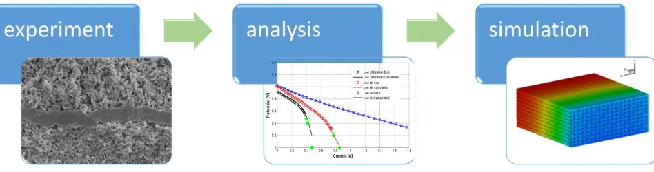
polarization analysis is then performed on the measured V-I curves to extract essential information of the cell under study, e.g. exchange current densities, ohmic resistance, etc. Then multi-physics numerical simulations are performed with parameters obtained by the empirical polarization analysis and refined by simultaneously matching polarization curves and impedance behaviors against experimental data sets. A sketch of the proposed physics based simulation methodology is depicted in Figure 1.
Figure 1. Sketch of the proposed physics based SOFC simulation and analysis procedure.
2.1 Empirical Polarization Analysis (EPA) of Measured V-I Curves
Empirical polarization analysis is applied to the measured V-I curves to extract essential information of the fuel cell under consideration. Parameter estimations derived from these simple experiments become a starting point in the multi-dimensional simulations.
The basic idea of polarization analysis is to find a function that estimates closely the measured V-I curves under different fuel and air utilization conditions. The total fuel cell operating voltage can be expressed as
V V IR
V Nernst total Nernst a c (1)
where the activation overpotential and concentration overpotential from anode and cathode are lumped into the terms a and c. The ohmic resistance R is obtained from 2D electric field simulation in which only the governing equations for the electric potential are solved. In such simulations, we employ variable electrical conductivity for nickel, LSM, and YSZ (see below).
1 {exp( ) exp[ (1 ) ]}]} ) 1 ( exp[ ) {exp( 2 2 2 0 0 RT nF RT nF i i c i i P i RT nF RT nF P P i i a a b L Fa a L Fa b a H a a a b O H a H a Fa
(2)
where
2
H
P is the bulk hydrogen concentration with unit atm, and
2 2 2 2 2
2 )/ (1 )/
1
( atm PH PN PH atm PH PN PH
c is a constant related to the bulk concentration.
These two coefficients will vary for different fuel utilization conditions. Eq.(2) captures both concentration effects and electrochemical reaction effects.
Similarly, a modified Butler-Volmer equation is used for oxygen reduction inside the active layer of the cathode which is given by
]} ) 1 ( exp[ ) {exp( 1 ]} ) 1 ( exp[ ) {exp( * 0 0 2 RT nF RT nF i i i RT nF RT nF P i i c c m L Fc c c c m O c Fc (3)
Here, reaction activity and concentration effects lump together into * 0c
i . MATLAB functions based on least square schemes are fitted to measured V-I curves for different utilization/supply conditions.
Analysis of the low fuel/air utilization cases, labeled as normal flow case in [3], generates the values of i0a, i0c, and b. In this case, the concentrations of air and fuel are so high that the utilization of air and fuel are very low when current density is small (10% at 0.5Voverpotential in experiments in [3]). Hence the following simplification is made for low utilization case:
1 / 2 2 H H P
P , / 1
2 2
O O P
P (4)
This assumption is only used in EPA, while MPNS adopts the generalized Butler-Volmer equation, i.e. Eq.(2) and Eq.(3). This protocol has been verified by the results of MPNS (see Appendix B). The steam concentration in the fuel stream can change significantly, hence it is retained in the anode equation as an unknown parameter.
The low air supply case is analyzed to estimate the exponent m and the low fuel supply case determines the value of a. The aforementioned analysis is based on the integral performances of SOFC, therefore an approximate average concentration profile of hydrogen and oxygen is assumed within the electrodes. The implications of this assumption are discussed in the results section.
2.2 Multi-Physics Numerical Simulation (MPNS)
In our previous work, similar numerical simulations were conducted using a simplified version of the current model to predict the polarization curve and impedance behavior for SOFCs [3, 14]. The whole electrodes were treated as active assuming that the well-percolated network of electrode phase and electrolyte phase extends throughout the electrode. The structural properties and effective diffusion coefficients were uniformly distributed. However, models which account for more realistic micro-structural configurations are indeed necessary to understand intricacies of SOFC performance. In the present study, we extended the multi-physics numerical simulations (MPNS) by incorporating realistic micro-structural and geometrical configurations and non-uniform property distributions. Furthermore, S.R. Pakalapati et al. [3] considered only V-I curves and Nyquist plots for the so called normal flow case with low utilization to support the assumption that the gas concentration at the counter electrode does not change the resistance of working electrode. In the current study, we consider the complete data sets, including polarization curves and impedance behavior for at least three cases (low utilization, low air supply, and low fuel supply case).
2.2.1 Governing Equations
Three contributions are considered in the charge conservation equation: specific capacitance, current associated with charge transport, and faradaic current, iF, from electrochemical reactions. The resulting charge conservation equations for electrode phases are given by [3, 8, 13, 14, 17, 24, 25]
F e e i
e eff
i t
C
) (
)
(
(5) and the charge conservation equation for electrolyte phase is
F i i e
i eff
i t
C
) (
)
(
(6)
In the bulk electrolyte, there is no interface between the electrode phase and the electrolyte phase, hence no faradaic current is present. Then the charge conservation equation Eq.(6) can be simplified to
0 )
(
ii (7)
Only diffusive gas-phase transport through porous media is considered, and it is modeled by Fick’s diffusion
D S
t
eff
)
( (8)
where Deff is the effective diffusion coefficient for species, is the molar concentration, and
) /(nF i
S F is the net source term due to electrochemical reactions (n2for H2, and n4 for O2).
2.2.2 Electrochemical Reactions
is expressed using Eq.(2) and Eq.(3) for the anode and cathode, respectively [5, 16, 33]. The anodic and cathodic overpotential, respectively, are defined by a (a i)(a i)eq and
eq i c i c
c ( ) ( )
.
2.2.3 Details of Mass Diffusion and Structural Properties
As presented in prior published work, the effective diffusion coefficient is calculated with consideration of Knudsen diffusion, binary diffusion, and tortuosity [34, 35].
1
,
1
1
Ki m
i i im n
eff
D D
y D
D
(9)
where Dij is binary diffusion and DKi is Knudsen diffusion. Details can be found in [34, 35]. In the present study, we chose nD 2.
Realistic distributions of properties are also considered and include the distribution of porosity, specific interface area between ion conducting phase and electron conducting phases, tortuosity, etc. Relations between interfacial area/tortuosity and porosity are considered as follows:
2/30 0 3
/ 2 0 0
int a
/
C C
/
a eff (10)
and
1/2 0 0 /
(11)Either the measured microstructure properties or those based on theoretical calculations (if available) are used [36].
The effective conductivity is also considered as
ieff
i(
V
i/
i)
, which means the effective conductivity is determined by the volume fraction Vi and tortuosity i of the electron-conducting or ion-conducting phase. For simplicity, the effective phase conductivity of the active layer is assumed to be identical to the support layer. For the cases considered, this is a reasonable assumption since the dominant contributor to ohmic resistance is the electrolyte.2.2.4 Numerical Algorithms
2.3 Details of the Proposed Procedure
Model parameters are generally coupled and consequently a given parameter will be sensitive to changes in other parameters. The specialized computational algorithm is therefore formulated as follows:
Step (i): Perform an integral polarization analysis of the three sets of measured V-I data to determine ohmic resistance (R), exchange current densities (i0a &i0c) and the exponents (a,b,m)
Step (ii): Refine exchange current densities (i0a &i0c) to match the polarization curve for the low utilization case.
Step (iii): Refine exponents (a,b,m) to match measured polarization curves at low current densities and impedance at OCV.
Step (iv): Adjust effective specific capacitance (Caeff &Cceff) to match the measured impedance curves.
Step (v): Adjust tortuosity(), hence effective diffusion coefficients(Deff), to improve agreements with experimental data for low air supply case and low fuel supply case.
3. RESULTS AND DISCUSSION
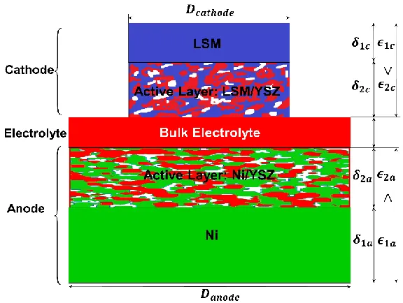
Figure 2. Two-dimensional sketch of a button cell in our simulations shown in this paper.
[image:8.596.154.442.381.598.2]
contributions of this layer to the polarization and impedance behavior of the cell are assumed to be limited to electron conduction and gas diffusion. The gas species are transported through the porous structure of both layers of each electrode. Therefore, governing equations of the whole button cell include the charge conservation within both electrodes and electrolyte and species transport within porous electrodes.
First, the methodology, which combines experiments, polarization analysis, and numerical simulation, is applied to the button cell. Three different utilization conditions are considered, low air/fuel utilization (LU) case, low air (LA) supply case, and low fuel (LF) supply case. Both polarization curves and impedance behaviors for three different fuel/air flow conditions are calibrated against experimental data. Then two more studies are presented to demonstrate that these three fuel/air flow conditions are leveraged to produce a complete set of experimental data.
Table 1 lists the supply conditions in air and fuel streams in the experiments used. In this study, the water contained in the air stream is neglected. The thickness of the full button cell is 960m, consisting of 900m anode, 10m electrolyte, and 50m cathode. The thickness of the active layer is
m
30 for the anode and 30m for cathode. Here, we want to point out that the anode thickness was
m
[image:9.596.45.537.431.490.2]250 in the simulations of [3] which was not addressed explicitly. In that study, the numerical algorithm became unstable for a thicker anode. In the present study, we have resolved this issue by modifying the code with arbitrary mesh sizes in electrodes.
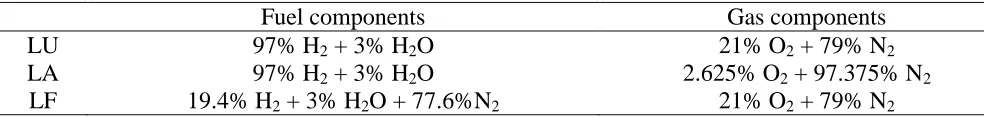
Table 1. Supply conditions in the experiments for different utilization cases.
Fuel components Gas components
LU 97% H2 + 3% H2O 21% O2 + 79% N2
LA 97% H2 + 3% H2O 2.625% O2 + 97.375% N2
LF 19.4% H2 + 3% H2O + 77.6%N2 21% O2 + 79% N2
3.1 Calibration for a Button Cell 3.1.1 Polarization Analysis
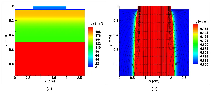
The ohmic resistance is obtained from 2D electric field simulations in which only the governing equations for the electric potential are solved. In these simulations, we use variable electric conductivity for nickel, LSM, and YSZ. Figure 3 shows the variable conductivity and contours of predicted current flow due to ohmic resistance. The calculated ohmic resistance is 0.41.
current curves from our analysis and the comparison against experimental measurements, in which good agreement can be observed.
Figure 3. Two-dimensional simulation of electric potential and current. (a) cell components and electric conductivity contours, (b) current density distribution.
Table 2. Essential cell information obtained from polarization analysis of experiments for different utilization cases.
variables values from EPA refined values in simulations
a
i0 (Am3) 8
10 29 .
1 7.0108
c
i0 (Am3) 8
10 02 .
1 2.66108
a 1.66 0.425
b 0.34 0.75
m 0.46 0.25
[image:10.596.79.517.132.322.2] [image:10.596.45.541.425.731.2]
3.1.2 Calibration of Simulations against Experiments
[image:11.596.46.552.159.424.2]The parameters used in the multi-dimensional simulations are summarized in Table 3. Table 3. Summary of parameters used in our multi-physics simulations of button cell.
Parameters Values
Thickness of anode(m) 900
Thickness of anode(m) 50
Thickness of anode(m) 10
Anode conductivity(1m1) 4.63103 Electrolyte conductivity(1m1) 0.4
Cathode conductivity(1m1) 6.34103 Reference specific capacitance at Ni/YSZ interface(Fm3) 1.43108
volumetric exchange current density in anodei0a (Am3) 8
10 0 .
7
exponent 'a' in the anode exchange current relation 0.425 exponent 'b' in the anode exchange current relation 0.75
Reference specific capacitance at LSM/YSZ interface(Fm3) 3.075107 volumetric exchange current density in cathode i0c (Am3) 8
10 66 .
2
exponent 'm' in the anode exchange current 0.25
Porosity in support layer 0.48
Porosity in active layer 0.23
[image:11.596.62.540.455.696.2]
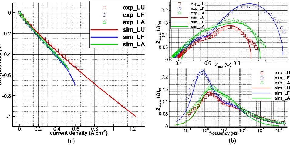
The low utilization case is first simulated with the values from polarization analysis, and the parameters are refined to match the experimental measurements. Boundary conditions shown in Table 1 are then altered for the low air supply case and the low fuel supply case. Figure 5 depicts the voltage-current curves and the corresponding impedance curves. The comparison shows good agreement between simulated and experimental results, and verifies the capability of the numerical tool accuracy. Data presented in Table 2 indicate that proper parameter evaluation requires input from both the VI analysis and the impedance simulation. As per the simulation protocol, approximate values can be obtained for the exchange current assuming uniform concentration profiles. The approximate parameter values are then used as a starting point in the multi-physics simulations, which allow more realistic concentration profiles (see Figure 6, 7, and 8). The results indicate sensitivity to the assumed concentration profile, and the modeled frequency response depicted in the Bode plots is related to the concentration effects via parameters a, b, and m(see Eq.(2) & (3)).
The simulation first determines the effective specific capacitance by matching the impedance curve for the low utilization case. Then for low air supply and low fuel supply case, the characteristic frequency is only related to concentration exponents. Therefore, the exponents are found by comparing the characteristic frequencies at low utilization case and high utilization cases. However, polarization analysis alone cannot determine these exponents accurately.
3.2 Further Validation of Proposed Model
The authors believe that a rigorous numerical model should predict the right physical processes occurring within the SOFC besides the overall performance. Therefore, in this section, we use the aforementioned calibrated numerical model to predict the details of processes within a button cell, and compare our predictions with those in the literature to further build confidence in our model. To this end, the species concentration profiles and current distribution, the cell performance of cell under various working loads, and the influence of cell geometry are investigated.
3.2.1 Details of Processes Occurring in SOFCs
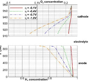
Figure 6. Simulated concentration profiles of hydrogen and oxygen within the electrodes for different total overpotentials for low utilization case.
[image:13.596.158.452.71.339.2] [image:13.596.157.454.395.663.2]
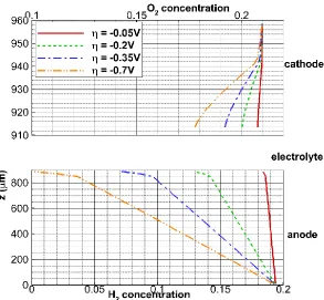
Figure 8. Simulated concentration profiles of hydrogen and oxygen within the electrodes for different total overpotentials for low fuel supply case.
Figure 9. Simulated current distribution (a) and concentration contours of hydrogen (red) and oxygen (blue) (b) for low utilization case with total1.0V which corresponds to the limiting current.
[image:14.596.157.450.68.339.2] [image:14.596.57.519.392.636.2]
the whole anode cross-section. Contour plots of hydrogen and oxygen are also shown in Figure 9(b). The contour plots of hydrogen in the anode reveal a nearly linear gradient perpendicular to the electrode/electrolyte interface within the area defined by the cathode, and a steep gradient in the radial direction. Despite the high flux of hydrogen to the anode/electrolyte zone opposite the cathode edge, the current density in this zone is smaller than in the area closer to the center of the cell. It is hard to measure these profiles inside the porous electrode in the experiments, however, similar distribution profiles can be found in simulations about anode-supported SOFC button cell with same geometry but different dimensions [42-44].
3.2.2 Prediction of Performance at Working Loads
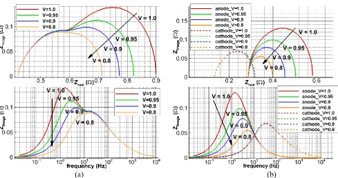
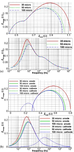
Figure 10. The simulated impedance behavior of button cell at different working loads, (top): Nyquist plots, (bottom) Bode plots, (a) impedance of whole cell, (b) impedance contributions from electrodes.
[image:15.596.55.544.258.516.2]
characteristic frequency approaches that of the cathode. This result is a consequence of the generation of relatively high water concentrations in the active layer of the anode with current flow. The effects of increasing water content arise from the second term in brackets with exponent bin Eq.(2). H. Zhu and R. J. Kee et al. [11] investigated the impedance of a button cell for various working loads utilizing H2 and CO as fuel. These authors observed reduced cell resistance as current density increased,
although there was only one arc for H2 cases. They attributed this phenomena to the high concentration
of H2O at large current density when H2is used as fuel. Our results and conclusions are consistent with
simulated cases with H2 in [11].
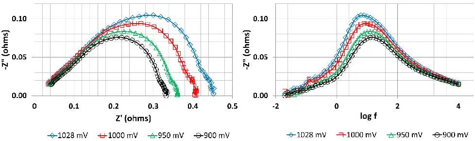
Although we did not perform such kind of study for the button cell mentioned in [3], H. Finklea et al. presented measurements from another button cell, which was manufactured by the same company as for the cell investigated in our study. It is expected that the trends from these two cells should be the same. Figure 11 shows the measured overall impedance behavior under different cell voltages. It can be observed that the low frequency arc changes significantly with cell voltage, which is associated to anode side consistent with our simulations as seen in Figure 10. Therefore, it may be concluded that our calibrated model is consistent with experimental observations on a similar cell for the performance at different working loads.
Figure 11. Measured button cell impedance under different cell voltages (1028mV, 1000mV, mV
950 , and 900mV) for low utilization cases.
3.2.3 Effects of Active Layer Thickness
[image:16.596.53.542.369.515.2]
polarization resistance on the active layer thickness is somewhat weaker than for the anode. For the anode part, we also observe in the simulations that the impedance does not change beyond an active layer thickness of approximately100m.
Figure 12. The simulated impedance behavior of button cell for different thicknesses of anode active layer. Total thickness of anode is900m, and the active layer thickness under study is30m,
m
[image:17.596.170.431.132.665.2]
Figure 13. The simulated impedance behavior of button cell for different thicknesses of cathode active layer. Total thickness of cathode is50m, and the active layer thickness under study is20m,
m
[image:18.596.149.453.68.693.2]
Predicting the influence of cell thickness on its performance is a good test case for model validation. This kind of study can be found in numerous experimental and theoretical studies [44-49]. Here, we compare the cathode thickness study (see results shown in Figure 13) with those in [45]. In [45], the whole cathode was made as active layer, and the authors also claimed better performance with thicker cathode. For the anode side, although the thickness of anode active layer in the literature varies, the results and conclusions in [46-49] are still applicable. It can be summarized that the active layer can not only increase the cell performance by adding more active zones, but also at the same time increase the resistance due to gas transport in porous media. Therefore, the cell performance may vary depending on the competition of these two components [44, 46-49]. The thickness of anode active layer used in our study is closer to the study in ([46], [47]) which showed improved performance with thicker anode active layer.
3.3 Consequences of Using Partial Data Sets
With all the previous calibration and validation study, we can conclude that our model can reveal the correct physics within SOFC after being calibrated using polarization curves and impedance behavior for three different utilization conditions. As one of the purposes of the present study, we would like to know if the model can predict the physics correctly when it is calibrated using only impedance data or only polarization data. In other words, we would like to find out the minimum requirements for data sets from experiments which can be used to calibrate a numerical model. To this end, we investigate the effects of using partial data sets, e.g. the calibration of the model using impedance data only or polarization data only.
Figure 14(a) shows simulation results with only impedance curves being calibrated. One set of simulation results (dotted line) are the calibrated results shown in Figure 5(b), while the other set (dashed line) shows the results with different values of tortuosity. The impedance behavior at open circuit voltage is not affected by the tortuosity because the utilization of gas and fuel is extremely small in such circumstances. However, as shown in Figure 14(b), the limiting current is reduced due to the reduction of the effective diffusion coefficient in Eq.(9) when we increase the tortuosity. This means that the value of tortuosity, hence the effective diffusion coefficients, cannot be calibrated when only impedance behavior is used as the targeted calibration data. This indicates that this partially calibrated model can only be used to investigate impedance behavior. For example, it is not appropriate to study species distribution by using this partially calibrated model. As mentioned in the methodology section, the diffusion coefficients are determined by matching the limiting currents of LA and LF cases. Obviously, if LA case is not included in the calibration processes, then the transport of gas species in cathode will be different from the realistic operating conditions. Similar conclusions can be made for anode side if LF case is not used.
Figure 14. Two sets of simulation results with only impedance behavior being calibrated. (a) calibrated impedance behavior at OCV, (b) corresponding polarization curves with determined properties. The difference of properties is *2. The corresponding experimental data can be
[image:20.596.54.541.72.323.2]found in Figures 5 (symbols).
Figure 15. Two sets of simulation results with only polarization curves being calibrated (a) calibrated polarization curves, (b) corresponding impedance behavior at OCV with determined properties. The difference of properties is eff
anode anode C
C* 2 and eff
cathode cathode C
[image:20.596.57.541.408.658.2]
The impedance response is a strong function of eff
C , and the location, magnitude, and peak frequency of the distinctive arcs change significantly. It can be concluded that this partially calibrated model is not suitable in analysis of anode and cathode impedance separately.
Using these two cases, we demonstrate that both polarization curves and impedance behavior are indispensable and should be used together. By considering anode, cathode, and overall cell performance as well as polarization curves and impedance behavior, at least three different air/fuel flow conditions are needed to produce a set of complete data for better understanding, hence for developing models with better physics, of the processes occurring within SOFCs.
4. CONCLUSIONS
In the present study, we present a procedure for performance analysis of solid oxide fuel cells whereby experiments and simulations are used simultaneously to supplement each other. Experimental data are analyzed to extract essential information of the fuel cell model, and estimated values are refined with detailed multi-physics simulations. This proposed tool is used to study the polarization curves and impedance behavior of a button cell with asymmetric configuration for different air/fuel utilization/supply conditions. The model is further validated by investigating the physical processes within the cell, including species and current distribution, performance at operating conditions, and influences of cell geometry. It is demonstrated that, in order to correctly assess the cell performance behavior, it is necessary not only to analyze the V-I curve alone, but also the details of the impedance measurements including Nyquist and Bode plots both in simulations and experiments. The present study also demonstrates that at least three different air/fuel flow conditions are needed to produce a set of complete data for better understanding of the processes occurring within SOFCs. Parametric study shows that the simultaneous calibration of polarization curves and impedance behavior is necessary to analyze the properties of SOFC. Comparison of current simulation results with many experimental and theoretical/computational studies published in the literature reveals that the proposed modeling procedure is reliable.
ACKNOWLEDGEMENT
Nomenclature
eff
C aintCDLeffective specific capacitance(Fm3)
symmetry factor, which is assumed to be 0.5 in this paper
n number of exchanged electrons in charge-transfer step which is
2
in this papere
electric potential of electron-conducting phase (V)
i
electric potential of ion-conducting phase (V)
e
electric conductivity of electron-conducting phase (1m1)
i
electric conductivity of ion-conducting phase (1m1)
F
i volumetric faradaic current density (Am3)
porosity of porous electrode
0
reference porosity of porous electrode
int
a volumetric interface area between electrode and electrolyte phase (m2m3)
0
a reference interface area between electrode phase and electrolyte phase (m2m3)
DL
C area-specific double-layer capacitance(Fm2) eff
C0 reference specific capacitance( ) 3
m F
tortuosity of porous electrode
0
reference tortuosity of porous electrode
molar concentration of species (molm3)
eff
D effective diffusion coefficient of species in porous media(m2s1)
S consumption/production rate due to electrochemical reactions (m2s1)
c a i
c a
, overpotential (V)
eq
electric potential in equilibrium condition (V)
Appendix A
Derivation of Polarization Model
The formula of polarization model used for anode can be derived from generalized Butler-Volmer equation, Eq.(2). The details are as follows
1 {exp( ) exp[ (1 ) ]}]} ) 1 ( exp[ ) {exp( ) 1 1 ( 1 ]} ) 1 ( exp[ ) {exp( ) 1 ( 1 1 ]} ) 1 ( exp[ ) {exp( 1 ]} ) 1 ( exp[ ) {exp( ]} ) 1 ( exp[ ) {exp( 2 2 2 2 2 2 2 2 2 2 2 2 2 2 2 2 2 2 2 2 0 0 0 0 0 0 RT nF RT nF i i c i i P i RT nF RT nF i i P P i i P i RT nF RT nF i i P P i i P i RT nF RT nF P P P P P P i RT nF RT nF P P P P P i RT nF RT nF P P i i a a b L Fa a L Fa b a H a a a b L Fa H N a L Fa b a H a a a b L Fa H N a L Fa b a H a a a b H N H a H H b a H a a a b H O H a H H b a H a a a b O H a H a Fa
(A.1)
In the above derivation, the relation between concentration of hydrogen and limiting current density is used that is
L Fa H H i i P P 1 2
where iL is limiting current density.
Similarly, we can derive the polarization model for cathode from Eq.(3)
]} ) 1 ( exp[ ) {exp( 1 ]} ) 1 ( exp[ ) {exp( 1 ]} ) 1 ( exp[ ) {exp( ]} ) 1 ( exp[ ) {exp( * 0 0 0 0 2 2 2 2 2 RT nF RT nF i i i RT nF RT nF i i P i RT nF RT nF P P P i RT nF RT nF P i i c c m L Fc c c c m L Fc m O c c c m O O m O c c c m O c Fc (A.3)
Appendix B
Justification of Assumption
In the proposed polarization model, we have the assumption Eq.(4) for low air/fuel utilization case. To investigate the effects of this assumption, we compared results from two simulations for low utilization case. The only difference between these two simulations is the Butler-Volmer equation used for
faradaic current. In one simulation (Simulation I), the generalized Butler-Volmer equation, Eq.(2) and Eq.(3), is used, while the other one (Simulation II) follows the assumption, Eq.(4), so that we have the following equations:
{exp( ) exp[ (1 ) ]}]} ) 1 ( exp[ ) {exp( ]} ) 1 ( exp[ ) {exp( 2 2 2 2 2 2 2 2 0 0 0 RT nF RT nF P P i RT nF RT nF P P P P i RT nF RT nF P P i i a a b O H a H a a a b O H a H H a H a a a b O H a H a Fa
(B.1)
{exp( ) exp[ (1 ) ]}]} ) 1 ( exp[ ) {exp( ]} ) 1 ( exp[ ) {exp( 2 2 2 2 2 0 0 0 RT nF RT nF P i RT nF RT nF P P P i RT nF RT nF P i i c c m O c c c m O O m O c c c m O c Fc
(B.2)
We then calculate the changes of current density and air/fuel concentrations with taking the simulation with generalized Butler-Volmer equations as the reference case:
II II
change(%) (B.3)
where
I is the result from Simulation I and
IIis the result from Simulation II.The change of current density is shown in Figure B.1, and changes of air and fuel concentration profiles are shown in Figure B.2 and B.3 respectively. It is seen that the differences are insignificant. Therefore, it can be concluded that the assumption Eq.(4) has little effect on the results for
0.5V , which is the case for low utilization. Hence, the assumption is valid. [image:25.596.172.411.534.700.2]
Figure B.2. Variation of air concentration profiles between the simulation with generalized Butler-Volmer equation (Simulation I) and simulation with assumption Eq.(4) (Simulation II) for low utilization case.
Figure B.3. Variation of fuel concentration profiles between the simulation with generalized Butler-Volmer equation (Simulation I) and simulation with assumption Eq.(4) (Simulation II) for low utilization case.
References
1. K. J. Yoon and S. Gopalan, J. Electrochem. Soc., 156 (2009) B311
[image:26.596.144.437.87.287.2] [image:26.596.140.426.393.589.2]
5. P. Costamagna, A. Selimovic, M. D. Borghi and G. Agnew, Chem. Eng. J. (Amsterdam, Neth.), 102 (2004) 61
6. A. Leonide, V. Sonn, A. Weber and E. Ivers-Tiffée, J. Electrochem. Soc., 155 (2008) B36 7. V. M. Janardhanan and O. Deutschmann, Z. Phys. Chem., 221 (2007) 443
8. W. G. Bessler, S. Gewies and M. Vogler, Electrochim. Acta, 53 (2007) 1782 9. W. G. Bessler, Solid State Ionics, 176 (2005) 997
10.W. G. Bessler, J. Electrochem. Soc., 154 (2007) B1186
11.H. Zhu and R. J. Kee, J. Electrochem. Soc., 153 (2006) A1765
12.H. Zhu, R. J. Kee, V. M. Janardhanan, O. Deutschmann and D. G. Goodwin, J. Electrochem. Soc., 152 (2005) A2427
13.H. Zhu and R. J. Kee, J. Electrochem. Soc., 155 (2008) B715
14.S. R. Pakalapati, K. Gerdes, H. Finklea, M. Gong, X. Liu and I. Celik, Solid State Ionics, 258 (2014) 45
15.M. Gong, R. S. Gemmen and X. Liu, J. Power Sources, 201 (2012) 204 16.W. G. Bessler, J. Electrochem. Soc., 153 (2006) A1492
17.S. Kakac, A. Pramuanjaroenkij and X. Y. Zhou, Int. J. Hydrogen Energy, 32 (2007) 761
18.K. Wang, D. Hissel, M.C. Péra, N. Steiner, D. Marra, M. Sorrentino, C. Pianese, M. Monteverde, P. Cardone and J. Saarinen, Int. J. Hydrogen Energy, 36 (2011) 7212
19.A. Leonide, Y. Apel and E. Ivers-Tiffée, ECS Trans., 19 (2009) 81
20.J. R. Ferguson, J. M. Fiard and R. Herbin, J. Power Sources, 58 (1996) 109 21.E. Achenbach, J. Power Sources, 49 (1994) 333
22.D. J. Hall and R. Gerald Colclaser, IEEE transactions on Energy Conversion, 14 (1999) 749 23.R. Bove and S. Ubertini, Modeling solid oxide fuel cells: methods, procedures and techniques,
Springer Science & Business Media (2008)
24.S. C. DeCaluwe, H. Zhu, R. J. Kee and G. S. Jackson, J. Electrochem. Soc., 155 (2008) B538 25.S. Gewies and W. G. Bessler, J. Electrochem. Soc., 155 (2008) B937
26.R. Ahmed and K. Reifsnider, Int. J. Electrochem. Sci, 6 (2011) 1159
27.G.B. Jung, L.H. Fang, C.Y. Lin, X.V. Nguyen, C.C. Yeh, C.Y. Lee, J.W. Yu, S.H. Chan, W.T. Lee, S.W. Chang and I.C. Kao, Int. J. Electrochem. Sci, 10 (2015) 9089
28.S. Su, X. Gao, Q. Zhang, W. Kong and D. Chen, Int. J. Electrochem. Sci, 10 (2015) 2487
29.A. Lasia, Electrochemical impedance spectroscopy and its applications, Springer, New York, US (2014)
30.J.R. Wilson, D.T. Schwartz and S.B. Adler, Electrochim. Acta, 51 (2006) 1389 31.S.B. Adler, ECS Trans., 58 (2013) 101
32.Y. Lu, C. R. Kreller, S. B. Adler, J. R. Wilson, S. A. Barnett, P. W. Voorhees, H.-Y. Chen and K. Thornton, J. Electrochem. Soc., 161 (2014) F561
33.X. Li, Principles of Fuel Cells, Taylor & Francis (2005)
34.F. N. Cayan, S. R. Pakalapati, F. Elizalde-Blancas and I. Celik, J. Power Sources, 192 (2009) 467 35.H. Yakabe, M. Hishinuma, M. Uratani, Y. Matsuzaki and I. Yasuda, J. Power Sources, 86 (2000)
423
36.M. Matyka, A. Khalili and Z. Koza, Phys. Rev. E, 78 (2008) 026306 37.H. L. Stone, SIAM Journal on Numerical Analysis, 5 (1968) 530
38.J. H. Ferziger and M. Peric, Computational methods for fluid dynamics, Springer Science & Business Media (2012)
39.S. R. Pakalapati, A new reduced order model for solid oxide fuel cells, Ph.D. Thesis, West Virginia University, Morgantown WV, USA (2006)
40.F. Elizalde-Blancas, Modeling issues for solid oxide fuel cells operating with coal syngas, Ph.D. Thesis, West Virginia University, Morgantown, WV, USA (2009)
43.Y. Shi, N. Cai, C. Li, C. Bao, E. Croiset, J. Qian, Q. Hu and S. Wang, J. Power Sources, 172 (2007) 246
44.Y. Shi, N. Cai and C. Li, J. Power Sources, 164 (2007) 639
45.A.V. Virkar, J. Chen, C.W. Tanner and J.W. Kim, Solid State Ionics, 131 (2000) 189
46.T. Suzuki, S. Sugihara, T. Yamaguchi, H. Sumi, K. Hamamoto and Y. Fujishiro, Electrochemistry Communications, 13 (2011) 959
47.T. Yamaguchi, H.Sumi, K. Hamamoto, T. Suzuki, Y. Fujishiro, J.D. Carter and S.A. Barnett, Int. J. Hydrogen Energy, 39 (2014) 19731
48.Y.M. Park, H.J. Lee, H.Y. Bae, J.S. Ahn and H. Kim, Int. J. Hydrogen Energy, 37 (2012) 4394 49.K. Chen, X.Chen, Z. Lü, N. Ai, X. Huang and W. Su, Electrochim. Acta, 53 (2008) 7825