Two-Fluid Eulerian-Eulerian CFD Modelling of Bubbly Flows Using an Elliptic-Blending Reynolds Stress Turbulence Model

This is a repository copy of

Two-Fluid Eulerian-Eulerian CFD Modelling of Bubbly Flows

Using an Elliptic-Blending Reynolds Stress Turbulence Model

.

White Rose Research Online URL for this paper:

http://eprints.whiterose.ac.uk/137752/

Version: Accepted Version

Proceedings Paper:

Colombo, M and Fairweather, M (2018) Two-Fluid Eulerian-Eulerian CFD Modelling of

Bubbly Flows Using an Elliptic-Blending Reynolds Stress Turbulence Model. In:

Proceedings of the 12th International ERCOFTAC Symposium on Engineering Turbulence

Modelling and Measurements. ETMM12: 12th International ERCOFTAC Symposium on

Engineering Turbulence Modelling and Measurements, 26-28 Sep 2018, Montpellier,

France. ETMM .

This is an author produced version of a paper published in Proceedings of the 12th

International ERCOFTAC Symposium on Engineering Turbulence Modelling and

Measurements.

eprints@whiterose.ac.uk https://eprints.whiterose.ac.uk/

Reuse

Items deposited in White Rose Research Online are protected by copyright, with all rights reserved unless indicated otherwise. They may be downloaded and/or printed for private study, or other acts as permitted by national copyright laws. The publisher or other rights holders may allow further reproduction and re-use of the full text version. This is indicated by the licence information on the White Rose Research Online record for the item.

Takedown

If you consider content in White Rose Research Online to be in breach of UK law, please notify us by

T

WO

-F

LUID

E

ULERIAN

-E

ULERIAN

CFD

M

ODELLING OF

B

UBBLY

F

LOWS

U

SING AN

E

LLIPTIC

-B

LENDING

R

EYNOLDS

S

TRESS

T

URBULENCE

M

ODEL

M. Colombo and M. Fairweather

School of Chemical and Process Engineering, University of Leeds, Leeds LS2 9JT, UK

M.Colombo@leeds.ac.uk

Abstract

In Eulerian-Eulerian two-fluid computational fluid dynamic (CFD) predictions of bubbly flows, the lateral void fraction distribution mainly results from a balance between the lift and wall lubrication forces. The impact of turbulence modelling on the void fraction distribution has not, however, been examined in detail. In this paper, this impact is stud-ied with an elliptic blending Reynolds stress turbu-lence model (EB-RSM) that resolves the near-wall region and includes the contribution of bubble-induced turbulence. Lift and wall lubrication forces are deliberately neglected. Comparisons against da-ta on bubbly flows in a pipe and a square duct show that the EB-RSM reproduces the lateral void frac-tion distribufrac-tion, including the peak in the near-wall region. The accuracy of this approach is comparable to best-practice high-Reynolds k- and second-moment turbulence closures that include lift and wall lubrication contributions. Overall, the role of the turbulence field is demonstrated to be signifi-cant in determining void fraction distributions, and has to be modelled appropriately if more accurate and consistent modelling of bubbly flows is to be achieved. In view of this, the present EB-RSM ap-proach is useful as a starting point to develop a more accurate and generally applicable set of clo-sure models for two-fluid CFD approaches.

1 Introduction

In multiphase gas-liquid bubbly flows, the bub-ble size distribution and the volume fraction of the gas phase strongly affect the flow of the continuous liquid phase and the design and operation of indus-trial equipment. The use of computational fluid dy-namic (CFD) models has made possible the calcula-tion of three-dimensional void fraccalcula-tion and interfa-cial area distributions whilst accounting for phe-nomena at much smaller length scales (Rzehak and Krepper, 2013; Colombo and Fairweather, 2016). For the prediction of flows of industrial-scale, Eu-lerian-Eulerian averaged two-fluid models have been the most frequent choice (Hosokawa and To-miyama, 2009; Colombo and Fairweather, 2015; Liao et al., 2015).

Eulerian-Eulerian two-fluid models treat the phases as interpenetrating continua and interphase exchanges are modelled by means of closure rela-tions. In closed ducts, the tendency of smaller bub-bles to migrate towards the walls and larger bubbub-bles to concentrate towards the centre is attributed to the action of the lift force, with the change in direction in the region of bubble diameters from 4 to 6 mm (Lucas et al., 2010). Consequently, in most CFD studies to date, the lateral void fraction distribution essentially results from a balance between the lift and wall lubrication forces acting on the bubbles. Although over the years numerous lift models have been developed, and many have been optimized to predict the wall-peak void fraction distribution, no general consensus on the most accurate model has yet been reached (Hibiki and Ishii, 2007). Addition-ally, an even larger number of slightly different models is available for the wall lubrication force (Antal et al., 1991; Hosokawa and Tomiyama, 2009; Rzehak and Krepper, 2013; Colombo and Fair-weather, 2015). However, more recently the near-wall peak of the void fraction profile was well-predicted even without lift and wall force contribu-tions by using a near-wall Reynolds stress model (RSM) (Ullrich et al., 2014). With the exception of a small number of contributions (Lopez de Bertodano et al., 1990; Mimouni et al., 2010), the role of the continuous phase turbulence has been rarely considered in previous works, in which mul-tiphase extensions of single-phase linear eddy vis-cosity models have generally been applied. Howev-er, recent direct numerical simulations (Santarelli and Frohlich, 2016) of fixed spherical bubbles in a shear flow found that, even with spherical bubbles, the lift force can become negative at high shear rates, demonstrating that the physical aspects of in-terfacial momentum transfer are more complex than generally envisaged. In addition, the presence of a liquid film between the bubble and the wall, which forms the basis of the wall lubrication theory, has also been questioned (Lubchenko et al., 2018).

con-tinuous phase turbulence on the lateral void fraction distribution is studied in a pipe and in a square duct, where the accuracy of lift and wall force models is much less well established. Results are compared to more standard high-Reynolds k- and Reynolds stress turbulence models. The action of the turbu-lence on the void fraction distribution and the bene-fits of high order turbulence modelling for overall two-fluid model accuracy and generality are ad-dressed.

2

Numerical model

In the two-fluid Eulerian-Eulerian model, a set of averaged continuity and momentum conservation equations is solved for each phase (Prosperetti and Tryggvason, 2007; Yeoh and Tu, 2010). Turbulence is resolved in the continuous phase using the EB-RSM (Manceau, 2015) that allows solution of the turbulence field up to the near-wall region. The transport equations of the Reynolds stresses are based on the corresponding single-phase formula-tion, and the pressure-strain relation is modelled us-ing the so-called “SSG model” (Speziale et al., 1991):

(1)

In the previous equation, k is the turbulence ki-netic energy, the turbulence energy dissipation rate and aij the components of the anisotropy tensor. P is the turbulence production and Sij and Wij are the strain rate and the rotation rate tensors, respectively. Near the wall, the SSG model is blended with a formulation that reproduces the near-wall asymptot-ic behaviour of the turbulent stresses:

(2)

Transition from the near-wall model in Eq. (2) to weakly inhomogeneous behaviour away from the wall is ensured by the elliptic relaxation function EB, which is obtained by solving an elliptic relaxa-tion equarelaxa-tion:

(3)

(4)

where L is the turbulence length scale. More details on the EB-RSM formulation can be found in Manceau (2015). The bubble contribution to the

continuous phase turbulence is accounted for with specific source terms that consider the conversion of energy lost by the bubbles to drag into turbulence kinetic energy in the bubble wakes (Rzehak and Krepper, 2013):

(5)

In Eq. (5), Fd is the drag force, Ur the relative

ve-locity and KBI is introduced to account for the mod-ulation of the turbulence source. In the turbulence energy dissipation rate equation, the bubble-induced source is expressed as the corresponding turbulence kinetic energy source term multiplied by the time-scale of the bubble-induced turbulence BI:

(6)

In multiphase turbulence, the bubble-induced turbulence timescale should be related to the shear-induced turbulent eddy lifetime as well as bubble length and velocity scales. The mixed timescale proposal from Rzehak and Krepper (2013) is adopt-ed, where the velocity scale is derived from the square root of the liquid turbulence kinetic energy and the length scale from the bubble diameter. C,BI is fixed to 1 and KBI is fixed to a value of 0.25, which provided good agreement over a large data-base of bubbly flows (Colombo and Fairweather, 2015). The bubble-induced turbulence model is im-plemented in the EB-RSM by splitting the contribu-tion amongst the normal Reynolds stress compo-nents. The performance of the EB-RSM is com-pared against high-Reynolds number multiphase formulations of the k- and RSM turbulence models (CD-adapco, 2016).

For the interfacial momentum transfer closures, the drag force is accounted for with the model of Tomiyama et al. (2002) and the turbulent dispersion force with the approach of Burns et al. (2004). In the high-Reynolds number models, the lift force is also included using a constant value of the lift coef-ficient CL = 0.1 (Colombo and Fairweather, 2015), and the wall force is modelled following Antal et al. (1991). As mentioned in the introduction, these two forces are neglected in the EB-RSM to highlight the impact of the turbulence field on the lateral void fraction distribution.

mesh close to the wall. Mesh-independent solutions were achieved with grids having the centre of the first cell located at a non-dimensional wall distance of 1-1.5, and the number of cells equal to 20,800 and 1,280,000 for the pipe and duct flow, respec-tively.

At the inlet, constant phase velocities and void fractions were imposed, together with an imposed pressure at the outlet. The no-slip boundary condi-tion was used at the wall. The average bubble diam-eter was considered constant and taken equal to av-erage measurements from the Hosokawa and Tomi-yama (2009), at 3.66 mm, and Sun et al. (2014), at 4.25 mm, experiments. Unfortunately, no additional detailed measurements of the average bubble di-ameter evolution and space distribution are availa-ble for the experiments considered. Second-order upwind schemes were used to discretize the convec-tive terms. Strict convergence of residuals was en-sured and the mass balance was checked to have an error always less than 0.1 % for both phases.

3

Results and discussion

In this section, numerical simulations are com-pared against experiment 4 of Hosokawa and Tomi-yama (2009) in an air-water bubbly pipe flow, and the experiment at jl = 0.75 m s-1 and ja = 0.09 m s-1 in a square duct from Sun et al. (2014).

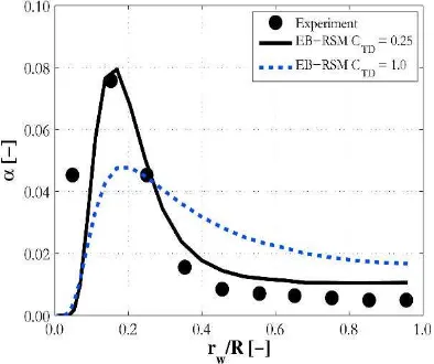
The void fraction radial profile predicted by the EB-RSM for the Hosokawa and Tomiyama (2009) experiment is shown in Figure 1, as a function of the non-dimensional radial distance from the wall rw/R. The wall-peaked void fraction profile, which is a distinctive feature of bubbly flows in pipes, is obtained even if lift and wall lubrication forces are neglected. When this is the case, the steady momen-tum balance in the radial direction for the liquid phase reduces to:

(7)

A similar balance can be written for the gas phase. Combining the two and neglecting turbulence stresses in the gas phase in view of the very low density ratio in gas-liquid bubbly flows, the follow-ing equation governfollow-ing the void fraction distribution is obtained:

(8)

From Eq. (8), turbulence in the liquid phase im-pacts the void fraction distribution and is responsi-ble for the preferential accumulation of bubresponsi-bles near the wall. In more detail, the gradient in the liq-uid phase radial turbulent stress generates a corre-sponding radial pressure gradient in the flow (Fig-ures 2 and 3) that pushes the bubbles towards the lower pressure region near the wall. There, pressure increases again approaching the wall as a conse-quence of the radial turbulent stress becoming zero. Therefore, although the wall force is neglected, fur-ther movement of the bubbles towards the wall is prevented and the wall-peaked void profile is ob-tained. Obviously, an accurate definition of the void fraction profile near the wall needs the turbulence field in that region to be finely resolved. To do so, a turbulence model able to resolve the flow field down to the viscous sub-layer is necessary.

Figure 1: Radial void fraction profile compared with Hosokawa and Tomiyama (2009) experiment.

Figure 2: Radial profile of the r.m.s of the turbulent radial velocity fluctuations compared with Hosokawa

Figure 3: Calculated radial profile of the pressure field for the Hosokawa and Tomiyama (2009)

experiment.

In Figure 1, the value of the peak is underesti-mated if the standard turbulent dispersion coeffi-cient CTD = 1.0 is used. Consequently, an excessive amount of void fraction is predicted in the centre of the pipe. More accurate predictions are obtained by reducing the turbulent dispersion coefficient to CTD = 0.25. It is, however, important to point out that it is not suggested that the turbulent dispersion force be optimized on a case-by-case basis. In this paper, the objective is to highlight the impact of the turbu-lence model predictions on the void fraction distri-bution and, to do so, other radial forces have been neglected. However, the lift force will also have a significant impact, and it should not be neglected in any general CFD modelling of bubbly flows. Cou-pling the EB-RSM model with a proper lift force model will indeed be a primary objective of future work. In view of this, the use of a reduced CTD il-lustrates that predictions using CTD = 1.0 can be fur-ther improved by including additional radial forces such as lift.

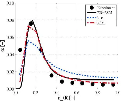
Results from the EB-RSM are comparable with, and superior to, predictions obtained with the high-Reynolds number k- and high-Reynolds stress turbu-lence models (Figure 4), which include both lift and wall lubrication forces.

Figure 5 shows how predictions of the turbu-lence kinetic energy are improved near the wall when using the EB-RSM as compared to the high-Re formulations. Properly accounting for the bub-ble-induced contribution (Eqs. (5) and (6)) also leads to accurate predictions in the centre of the pipe. Figure 6 demonstrates the ability of the EB-RSM model to reproduce the anisotropy of the tur-bulence field and, therefore, the impact of the radial pressure gradient on the void fraction distribution.

Figure 4: Radial void fraction profile compared with Hosokawa and Tomiyama (2009) experiment.

Figure 5: Radial profile of the turbulence kinetic energy compared with the Hosokawa and Tomiyama

(2009) experiment.

Figure 6: Radial profiles of the r.m.s. of the turbulent velocity fluctuations compared with the Hosokawa

and Tomiyama (2009) experiment.

experi-mentally by Sun et al. (2014). The pressure distribu-tion in the duct cross-secdistribu-tion from the EB-RSM is shown in Figure 7, where a minimum in the corner of the duct is clearly visible. Similarly to what was reported for the pipe flow, the bubbles preferentially accumulate in this low pressure region and the void fraction distribution shows a maximum correspond-ing with the corner of the duct (Figure 8).

Figure 7: Pressure field for the Sun et al. (2014) experiment calculated with the EB-RSM.

Figure 8: Void fraction field for the Sun et al. (2014) experiment calculated with the EB-RSM.

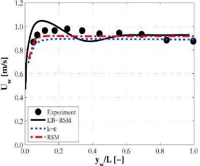
Figures 9 and 10 compare mean liquid velocity and void fraction predictions from the EB-RSM and the high-Reynolds number models. Figure 9 shows the liquid velocity profile on a line parallel to one of the lateral walls and as function of the non-dimensional distance from the perpendicular wall yw/L. Good agreement is obtained with all the mod-els, except for a small oscillation in the EB-RSM profile. This is probably due to an excessive sensi-tivity to the behaviour of the pressure field caused by the absence of any other radial forces. Figure 10 provides profiles of the void fraction along the di-agonal of the duct and as a function of the non-dimensional distance from the duct corner dw/D, where D is the diagonal length. Remarkably, the void fraction distribution is well-predicted by the EB-RSM. Therefore, although the model neglects

any lift and wall lubrication contributions, the dis-tinctive features of the void distribution, and the void peak in the corner of the duct, are correctly predicted by properly resolving the turbulence field and the near-wall region. Results are also in agree-ment with the high-Re number predictions, but the EB-RSM is the only model to predict the slight dip in the void fraction after the peak and the subse-quent further increase towards the centre of the duct.

Figure 9: Liquid velocity predictions compared with the Sun et al. (2014) experiment.

Figure 10: Void fraction predictions compared with the Sun et al. (2014) experiment.

3

Conclusions

There-fore, turbulence action has to be taken into account and reliably predicted and at least a second-moment turbulence closure that finely resolves the near-wall region is desirable. The lift force is still expected to play a prominent role and a proper lift model will be added in future work aimed at developing a two-fluid CFD model of improved accuracy and reliabil-ity.

Acknowledgements

The authors gratefully acknowledge the financial support of the EPSRC under grant EP/K007777/1, Thermal Hydraulics for Boiling and Passive Sys-tems, and EP/M018733/1, Grace Time, part of the UK-India Civil Nuclear Collaboration.

References

Antal, S.P., Lahey, R.T. and Flaherty, J.E. (1991), Analysis of phase distribution in fully developed laminar bubbly two-phase flow, Int. J. Multiphase Flow, Vol. 17, pp. 635-652.

Burns, A.D., Frank, T., Hamill, I. and Shi, J.M. (2004), The Favre averaged drag model for turbulent dispersion in Eulerian multi-phase flows, Fifth International Conference on Multiphase Flows, Yokohama, Japan, May 30 - June 4.

CD-adapco (2016), STAR-CCM+® _{Version 10.04}

User Guide.

Colombo, M. and Fairweather, M. (2015), Multiphase turbulence in bubbly flows: RANS simulations, Int. J. Multiphase Flow, Vol. 77, pp. 222-243.

Colombo, M. and Fairweather, M. (2016), RANS simulation of bubble coalescence and break-up in bubbly two-phase flows, Chem. Eng. Sci., Vol. 146, pp. 207-225.

Hibiki, T. and Ishii, M. (2007), Lift force in bubbly flow systems, Chem. Eng. Sci., Vol. 62, pp. 6457-6474.

Hosokawa, S. and Tomiyama, A. (2009), Multi-fluid simulation of turbulent bubbly pipe flow, Chem. Eng. Sci., Vol. 64, pp. 5308-5318.

Liao, Y., Rzehak, R., Lucas, D. and Krepper, E. (2015), Baseline closure model for dispersed bubbly flow: Bubble coalescence and breakup, Chem. Eng. Sci., Vol. 122, pp. 336-349.

Lopez de Bertodano, M., Lee, S.J., Lahey Jr., R.T. and Drew, D.A. (1990), The prediction of two-phase turbulence and phase distribution phenomena using a Reynolds stress model, J. Fluid Eng., Vol. 112, pp. 107-113.

Lubchenko, N., Magolan, B., Sugrue, R. and Baglietto, E. (2018), A more fundamental wall lubri-cation force from turbulent dispersion regularization for multiphase CFD applications, Int. J. Multiphase Flow, Vol. 98, pp. 36-44.

Lucas, D., Beyer, M., Szalinski, L. and Schutz, P. (2010), A new database on the evolution of air-water flows along a large vertical pipe, Int. J. Therm. Sci., Vol. 49, pp. 664-674.

Manceau, R. (2015), Recent progress in the development of the elliptic blending Reynolds-stress model, Int. J. Heat Fluid Flow, Vol. 51, pp. 195-220. Mimouni, S., Archambeau, F., Boucker, M., Lavieville, J. and Morel, C. (2010), A second order turbulence model based on a Reynolds stress approach for two-phase boiling flows. Part 1: Application to the ASU-annular channel case, Nucl. Eng. Des., Vol. 240, pp. 2233-2243.

Prosperetti, A. and Tryggvason, G. (2007), Computational methods for multiphase flow, Cambridge University Press, Cambridge, United Kingdom.

Rzehak, R. and Krepper, E. (2013), CFD modelling of bubble-induced turbulence, Int. J. Multiphase Flow, Vol. 55, pp. 138-155.

Santarelli, C. and Frohlich, J. (2016), Direct numerical simulations of spherical bubbles in vertical turbulent channel flow, Int. J. Multiphase Flow, Vol. 81, pp. 27-45.

Speziale, C.G., Sarkar, S. and Gatski, T.B. (1991), Modelling the pressure-strain correlation of turbulence: An invariant dynamical system approach, J. Fluid Mech., Vol. 227, pp. 245-272.

Sun, H., Kunugi, T., Shen, X., Wu, D. and Nakamura, H. (2014), Upward air-water bubbly flow characteristics in a vertical square duct, J. Nucl. Sci. Technol., Vol. 51, pp. 267-281.

Tomiyama, A., Celata, G.P., Hosokawa, S. and Yoshida, S. (2002), Terminal velocity of single bubbles in surface tension dominant regime, Int. J. Multiphase Flow, Vol. 28, pp. 1497-1519.

Ullrich, M., Maduta, R. and Jakirlic, S. (2014), Turbulent bubbly flow in a vertical pipe computed by an eddy-resolving Reynolds stress model, 10th International ERCOFTAC Symposium on Engineering Turbulence Modelling and

Measurements (ETMM 10), Marbella, Spain,

September 17-19.