THESES. SIS/LIBRARY R.G. MENZIES BUILDING N0.2 Australian National University Canberra ACT 0200 Australia
USE OF THESES
This copy is supplied for purposes of private study and research only. Passages from the thesis may not be copied or closely paraphrased without the
written consent of the author.
THE AUSTRALIAN NATIONAL UNMRSllY
Telephone: "61 2 6125 4631 Facsimile: "61 2 6125 4063
A comparison of combinatory methods and
GIS based MOLA (IDRISI®) for solving
Multi-Objective Land use Assessment and
Allocation Problems
By
Sunil Kumar Sharma
A thesis submitted for the degree of Doctor of Philosophy of
the Australian National University
The Australian National University
Canberra, Australia
Declaration
I declare that this thesis is based on my own research and it does not contain any material, published or submitted by another person except where duly acknowledged in the text.
£,
····~
Acknowledgements
I am very grateful to my supervisor Dr. Brian G. Lees (SRES, ANU) for his constant support, encouragement, and critical eye in completing my PhD. He is the first person who introduced me to the field of geographical information science in 1997. At that time I had not even dreamed of doing a PhD in this field. Thanks Brian, for helping me to find my career path. I am sincerely grateful to my advisors Dr. J. Walker (CSIRO) and, in particular, Dr. M. J. Hill (BRS) for their guidance, and encouraging comments on the drafts. My PhD would not have been completed without their invaluable support in all aspects of the research and writing.
I would like to thank the Federal Government of Australia for awarding me a International Post Graduate Research Scholarship (IPRS) and the Australian National University for the PhD Scholarship. I am also thankful to the Department of Forests, Nepal for approving study leave to undertake this opportunity. I am especially thankful to Prof. Kanowski (Head of School, SRES) for providing me this opportunity to pursue a PhD degree at SRES and also grateful for his constant support and encouragement to finish my PhD. I am very pleased to extend by my special thanks to Dr. Holzknecht (Academic Adviser, SRES) for providing tremendous help to improve the thesis to this standard.
their universities. I offer my appreciation to Dr Hom Pant, Dr Amrottam Shrestha, Dr
Pramod Adhikari and Rupen for their advice in my research. I am also thankful to my
colleagues, Adam, Bruce, Sanjeev, Paul and Houshang at Gl room in the Geography
Building for their friendship and support in my studies.
I am always grateful to Usha didi and her family for helping my family to settle in
Canberra and providing us guardianship. It was a great support, creating a happy environment for my research. Academic advice and support from her were also vital to
my PhD. The Australian-Nepal Friendship Society also played a great role by providing
a forum of all Nepalese and Australian friends of Nepal in Canberra and minimized
home sickness and cultural differences by organizing activities (Dashain, Tihar, New
Year Celebration) and frequent gatherings. I am also grateful to Indra and his family for their support to finish my studies.
It was my parents who dreamed to see me with a PhD degree. They supported me throughout my academic career by all means available to them, covering all financial
burdens even in a difficult economic situation. Unfortunately, it was too late when I got this opportunity for doing a PhD degree. My father, who always desired and dreamed to
see me with PhD, died six months before I got an offer letter for a PhD degree from the
ANU in Nov. 2002. My parents have always been behind my every success and also for
pursuing this degree and completing it. So I want to acknowledge them by dedicating this thesis to them.
Above all, my dear wife, Jamuna made it possible for me to complete my PhD by
providing continuous support and encouragement to finish it. My children, Suyasa
(daughter, 9 yrs) and Shorup (son, 4 yrs) were always very supportive towards my study
and agreed to remain at home on numerous occasions in order to allow me to complete
writing. They were really helpful to relieve my stress accumulated at the university after
coming back home. I would like to share this success with Jamuna, Suyasa and Shorup.
Finally, I would like to express my sincere thanks to all members of our family and all
Abstract
The aim of this study was to provide an informed choice among two combinatory
methods and GIS based MOLA module in IDRIS!® by comparing their performance in
solving a hypothetical Multi-Objective Land use Assessment and Allocation (MOLAA)
problem. Among the combinatory methods, Simulated Annealing and Tabu Search
algorithms were chosen for study. The application of Simulated Annealing has already been demonstrated in solving a MOLAA problem but Tabu Search has not been used to
a MOLAA problem before.
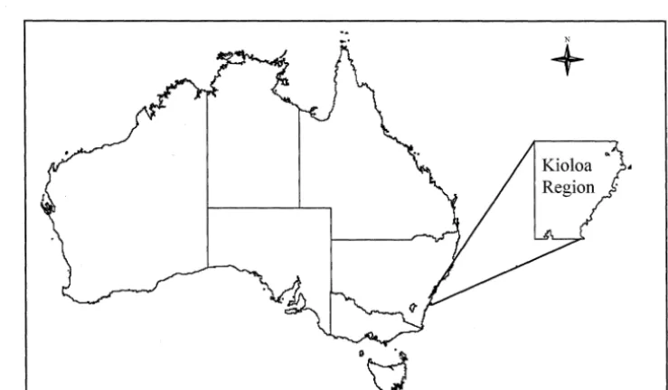
The Kioloa Region of New South Wales, Australia was chosen for designing a
hypothetical MOLAA problem due to availability and access to the digital datasets at
the Australian National University. The MOLAA problem was formulated for accomplishing six land use objectives by allocating the area to four land use types, that
is, conservation, agriculture, forestry and development, using altogether 1 7 criteria,
including 16 factors and one constraint. The criteria maps were classified in ordinal,
continuous and fuzzy scale and combined by using Weighted Linear Combination to
produce land use suitability models for each land use type. The ordinal and continuous
land use suitability models were used in solving the problem by applying the MOLA
module. In order to apply the combinatory methods, all three land use suitability
models, that is, ordinal, continuous and fuzzy, were transferred to cost suitability
models where the lowest cost value represented the best suitability and the highest cost
value represented the lowest suitability in the interval data set. Three initial input
solutions generated by the random, cheapest and greatest difference methods were used
for optimising by applying both algorithms.
Both combinatory methods maximized overall land use suitability with better spatial
compactness by allocating each land unit with the most suitable land use with the lowest
cost. At the land use level, MOLA exhibited a bias towards land uses with lower area
requirement and allocates more suitable land units to them. Though the MOLA module
is highly efficient in solving large grid MOLAA problem, the combinatory methods
deliver a solution close to the near-optimal solution with better compactness in an
acceptable time frame. Hence, the combinatory methods have been shown to be
The solutions were not significantly different at their mean cost functions between Simulated Annealing and Tahu Search at the appropriate parameters. Among the cost suitability models, both algorithms performed better in the fuzzy models in the large MOLAA problem. The initial input solution influenced the performance of the algorithms. The algorithms produced better results in the cheapest and greatest difference initial input solution in the medium grid MOLAA problem whereas the cost function was more improved using the random initial input solution in the large grid.
Although there is no significant difference in the mean cost functions between Simulated Annealing and Tahu Search, the previous one is found more efficient in solving large grid MOLAA problem. For the same values of compactness factors, Simulated Annealing produced more spatially compact land use allocation than Tahu Search. Thus decision makers/land use planners or consultants could obtain a better decision alternative to a land use allocation problem by applying Simulated Annealing with the recommended appropriate annealing schedule and initial input cost suitability model.
ANU BRS CDA CI CR CSIRO CSM DEM DTM GIS GRASS Ha HO IPA JMF M MCA MCE MCDA MCDM MCGDM MODM MOLA MO LAA NP-Hard
Acronyms
The Australian National University
Bureau of Rural Sciences
Concordance-Discordance Analysis
Consistency Index
Consistence Ratio
Commonwealth Scientific and Industrial Research Organization
Climatic Suitability Map
Digital Elevation Model
Digital Terrain Model
Geographic Information System
Geographic Resource Analysis Support System
Hectare
Hierarchical optimisation
Ideal Point Analysis
Joint Membership Function
Metre
Multi-Criteria Analysis
Multi-Criteria Evaluation
Multi-Criteria Decision Analysis
Multi-Criteria Decision Making
Multi-Criteria Group Decision Making model
Multiple Objective Decision Making
Multi-objective Land Allocation
Multi-objective Land use Assessment and Allocation
NSW
NSWNPWS
ooc
OSM
owe
PCA
RIW
SA
SDSS
SR
SSM
TS
New South Wales
New South Wales National Parks and Wildlife Service
Objectives-Oriented Comparison
Overall Suitability Map
Order Weight Combination
Principle Component Analysis
Relative Importance Weights
Simulated Annealing
Spatial Decision Support System
Similarity Relation Model
Soil Suitability Map
Glossary
Annealing schedule It comprises all the parameters used in Simulated Annealing such as cooling function, cooling rate, initial temperature, number of swaps per step and number of steps.
Cold swap The swapping of land uses between two cells decreases the cost function value.
Combinatory methods Those optimisation methods, which can solve combinatorial problems in an acceptable time frame.
Compactness function A function used in the cost minimization function in order to enhance spatial compactness.
Cooling function It is a mathematical rule or formula to reduce the initial control parameter or temperature in Simulated Annealing.
Cooling rate
Cost suitability model
Hot swap
It is the rate applied to reduce the initial control parameter or temperature in Simulated Annealing.
The models derived from land use suitability models where the lowest value represents the highest suitability and vice versa in interval scale.
The swapping of land uses between two cells increases the cost function value.
Initial control The initial value of temperature or control parameter used in parameter I temperature the Simulated Annealing.
Initial input solution
Land characteristics
Land unit
Land use suitability model
Land use type
Metropolis criterion
Neighbourhood solution
The feasible solution created for optimisation, using combinatory methods.
The physical attributes of land that may or may not favour a particular land use type.
It is represented by a cell or pixel with dimension 30 m by 30 metre in a raster data set.
It implies the classification of data sets using ordinal, continuous or fuzzy methods before deriving a land use suitability map.
It is the option to use desired use of land to achieve one or more objectives. For example, conservation, agriculture.
A criterion that probabilistically decides whether or not to accept a move with higher cost function in Simulated Annealing.
Simulated annealing
Swapping rate
Tabu length
Tabu list
Tabu Search
It is an approximation optimisation technique based on the physical process of annealing.
It is the total number of swapping of land uses between two randomly selected land use units in a step.
It specifies the size of a Tabu list or the number of iterations for restricting a 'Tabu' move.
A list of specified moves or solution not accessible for specified number of iterations.
Table of Contents
Declaration ... ii
Acknowledgements ... iii
Abstract ... v
Acronyms ... vii
Glossary ... ix
Table of Contents ... xi
List a/Tables ... xvi
List of Figures ... xix
Chapter 1 ... 1
INTRODUCTION ... 1
I. I Research problem ... I 1.2 Research objectives ... 7
I. 3 Implications of the research. ... 8
I. 4 Background concepts ... 9
1.4.1 Land and land use ... 9
1.4.2 Land valuation and land evaluation ... 10
1.4.3 Land capability and land suitability ... 11
1.4.4 Land use objectives and conflict ... 13
1.4.5 Land use planning and land use allocation ... 14
I. 5 Organization of the thesis ... 15
1.6 Papers from this thesis ... 17
Chapter 2 ... 18
APPROACHES TO MULTI-OBJECTIVE LAND USE DECISION-MAKING ... 18
2.1 Introduction ... 18
2. 2 Land use decision-making ... 18
2.3 A framework for land use decision-making ... 20
2.3.1 Problem Structuring ... 20
2.3.1.1 Stakeholders and decision makers ... 20
2.3.1.2 Land use objectives and land use (type) ... 22
2.3 .1.3 Land use evaluation criteria ... 22
2.3 .1.4 Spatial criteria in land use allocation ... 23
2.3 .2 Land use suitability assessment approaches ... 24
2.3.2.2 Taking account of factor weight ... 27
2.3.3 Decision support tool ... 36
2.3.3.1 Multi-criteria decision-making (MCDM) ... 36
2.3.3.2 GIS application in land use decision-making ... 42
2.4 Summary ... 47
Chapter 3 ... 49
METHODS FOR MULTI-OBJECTIVE LAND USE ALLOCATION ... 49
3.1Introduction ... 49
3.2 Combinatorial methods ... 49
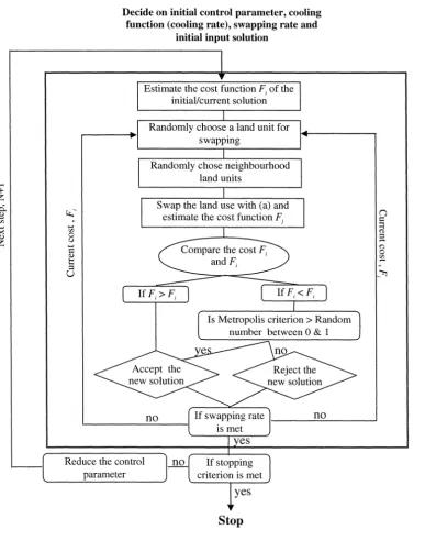
3.2.1 Simulated Annealing ... 50
3.2.1.1 Parameters for implementing Simulated Annealing Algorithm ... 54
3.2.1.2 Applying Simulated Annealing to a MO LAA problem ... 59
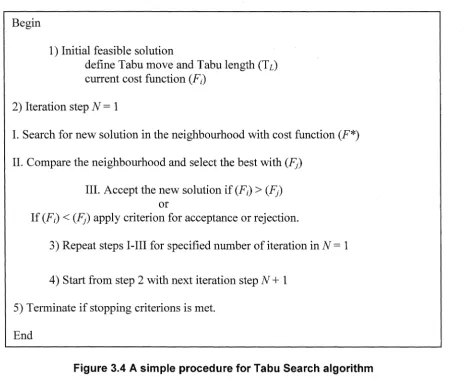
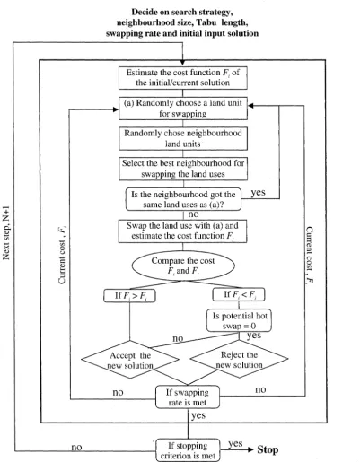
3.2.2 Tahu Search algorithm ... 61
3.2.2.1 Elements of Tahu Search ... 63
3.2.2.2 Applying of Tahu Search to a MO LAA problem ... 65
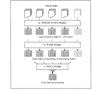
3.3 Multi objective land use allocation (MOLA) ... 66
3. 4 Summary ... 68
Chapter 4 ... 70
RESEARCH FRAMEWORK AND STUDY SITE ... 70
4.1 Introduction ... 70
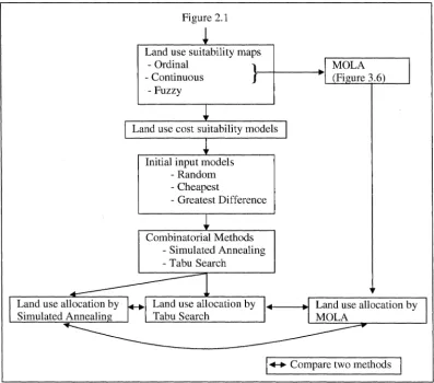
4.2 Research framework ... 70
4. 3 The Study site ... 7 4 4.3.1 Kioloa Region ... 75
4.3.1.1 Land use ... 75
4.3.1.2 Geology ... 76
4.3.1.3 Vegetation ... 76
4.3.2 The datasets for the Kioloa Region ... 76
4.3.2.1 Vegetation map ... 77
4.3.2.2 Digital Elevation Model and its derivatives ... 77
4.3.2.3 Geology dataset ... 78
4.3.2.4 Roads and tracks dataset ... 79
4.3.2.5 Park boundaries ... 79
4. 4 Summary ... 79
Chapter 5 ... 80
METHODOLOGY ... 80
5.2 Designing a hypothetical MOLAAproblemfor the Kioloa Region ... 80
5.2.1 Land use issues and objectives ... 80
5.2.2 Determining criteria for land use types ... 82
5.2.2.1 Conservation land use ... 84
5.2.2.2 Agriculture land use ... 84
5.2.2.3 Forestry land use ... 85
5.2.2.4 Development areas ... 85
5. 3 Land suitability assessment approach ... 86
5.3.1 Land use suitability models using ordinal - WLC ... 86
5.3.2 Land use suitability models using continuous - WLC ... 88
5.3.3 Land use suitability using fuzzy - WLC ... 89
5. 4 Land use input models for different methods ... 90
5.4.1 For MOLA ... 90
5.4.1.1 Ordinal land use suitability model.. ... 90
5.4.1.2. Continuous land use suitability model ... 91
5.4.2 For Combinatorial methods ... 91
5.5 Applying MOLA Module and Combinatory methods to the hypothetical MOLAA problem ... 96
5.5.1 MOLA module in IDRIS!® ... 96
5.5.2 Applying Combinatorial methods ... 97
5.5.2.1 Initial input solution for Combinatorial methods ... 97
5 .5 .2.2 Applying Simulated Annealing ... 100
5.5.2.3 Applying Tahu Search algorithms ... 105
5. 6 Summary ... 109
Chapter 6 ... 110
RESULT AND DISCUSSION I - APPL YING MOLA IN SOLVING A HYPOTHETICAL MOLAA PROBLEM ... 110
6.1 Results ... 110
6.1.1 Solving a hypothetical MOLAA problem using MOLA ... 110
6.1.1.1 Land use allocation for the ordinal land use suitability model.. ... 110
6.1.1.2 Land use allocation for continuous land use suitability model ... 114
6. 2 Discussion ... 115
6.3 Conclusion ... 117
6.4 Summary ... 118
Chapter 7 ... 119
7.1 Results ... 120
7 .1.1 Determining initial control parameter for Simulated Annealing ... 120
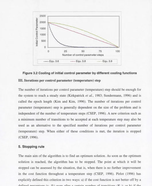
7 .1.2 Cooling function for Simulated Annealing ... 120
7 .1.3 Cost function minimization by different parameters ... 122
7.1.3.1 Influence of initial control parameter on cost function ... 123
7.1.3.2 Influence of cooling rate (CR) on the cost function ... 123
7.1.3.3 Influence of swapping rate (SR) on the cost function ... 126
7.1.4 Optimum cost function for different cost models ... 127
7.1.5 Assessing the performance of simulated annealing in solving a MOLAA problem ... 131
7.1.5.1 Analysing the spatial compactness without using the compactness function ... 131
7.1.5.2 Computation time ... 132
7 .1.6 Appropriate annealing schedule for Simulated Annealing in solving a MOLAA problem ... 133
7.1.7 Applying compactness function in solving a MOLAA problem ... 135
7.1.8 Appropriate initial input solution and cost model in solving the MOLAA problem ... 138
7. 2 Discussion ... 13 9 7.3 Conclusion ... 142
7.4 Summary ... 145
Chapter 8 ... 147
RESULTS AND DISCUSSION III - APPLYING TABU SEARCH TO THE HYPOTHETICAL MOLAA PROBLEM ... 147
8.1 Results ... 148
8.1.1 Influence of static and dynamic modes on cost function minimization .... 148
8.1.2 Influence of neighbourhood sizes on cost function minimization ... 149
8.1.3 Influence of Tahu length on cost function minimization ... 151
8.1.4 Influence of swapping rate on cost function minimization ... 151
8.1.5 Optimum cost function for different grid sizes and cost models ... 154
8.1.6 Assessing performance of Tahu Search in solving the MOLAA problem 157 8.1.6.1 Analysing the spatial compactness without compactness function ... 157
8.1.6.2 Computation time ... 157
8.1.7 Appropriate parameters for Tahu Search ... 159
8.1.8 Applying compactness function in the algorithm ... 160
8.1.9 Appropriate input model and cost model for Tahu Search ... 160
8. 2 Discussion ... 162
8. 4 Summary ... 166
Chapter 9 ... 168
COMPARING THE GIS BASED MOLA AND COMBINATORY METHODS ... 168
9.1 Results ... 168
9.1.1 Comparing the solutions to the MOLAA problem by Combinatory methods and MOLA module ... 168
9 .1.1.1 Cost function as a measure of overall of land use suitability ... 168
9.1.1.2 Spatial compactness a desirable criterion for land use allocation ... 172
9 .1.1.3 Computation time as a measure of efficiency of the methods ... 173
9 .1.2 Adding compactness function into the combinatory methods ... 173
9. 2 Discussion ... 17 4 9.3 Conclusion ... 177
9.4 Summary ... 178
Chapter 10 ... 179
CONCLUSIONS ... 179
References ... 184
Annex -1: An example of output summary from the Simulated Annealing ... 197
Annex - 2: An example of output summary from the Tahu Search ... 199
Annex - 3: An example of output file from the MOLA module ... 202
List of Tables
Table 1.1 MCDM techniques for solving single/multiple land use allocation problems. 5
Table 2.1 Scale for pair-wise comparison proposed by Saaty (1977) ... 29
Table 2.2 A Pair-wise comparison matrix for deriving relative weights ... 29
Table 2.3 Combinatory methods used for solving real world combinatorial optimization problems ... 42
Table 4.1 Area coverage of different land uses in the Kioloa region ... 75
Table 4.2 Summary of the datasets for the Kioloa region ... 76
Table 4.3 Distribution of geology type in the Kioloa Region ... 78
Table 5.1 Thresholds for criteria used for different land use types ... 83
Table 5.2 Criteria and attribute classification in ordinal scale for conservation ... 87
Table 5.3 Criteria and attribute classification in ordinal scale for agriculture ... 87
Table 5.4 Criteria and attribute classification in ordinal scale for forestry ... 87
Table 5.5 Criteria and attribute classification in ordinal scale for development use ... 87
Table 5.6 Criteria, their data types, range of values and fuzzy model applied with parameter values for different land use types ... 90
Table 5.7 Cost suitability values for small grid (10 by 10 cells) for all three cost models ... 93
Table 5.8 Cost suitability values for medium grid (100 by 100 cells) for all three cost models ... 93
Table 5.9 Cost suitability values for large grid (525 by 525 cells) for all three cost models ... 94
Table 5.10 Total and mean cost functions for different input solution and grid sizes for ordinal model ... 100
Table 5.11 Total and mean cost functions for different input solution and grid sizes for continuous model. ... 100
Table 5.12 Total and mean cost functions for different input solution and grid sizes for fuzzy model ... 100
Table 6.1 Rank values and spatial compactness for ordinal land use suitability model ... 111
Table 6.2 Distribution of rank values allocated to four land uses in a small grid by MOLA using ordinal land use suitability model ... 112
Table 6.3 Rank values and spatial compactness for continuous land use suitability model ... 115
Table 6.4 Distribution of rank values for four land use types in a small grid for continuous land use suitability model ... 115
Table 7.2 Initial control parameters for ordinal model at different hot-swap acceptance percentages ... 120 Table 7.3 Initial control parameters for continuous model at different hot-swap
acceptance percentages ... 120 Table 7.4 Initial control parameters for fuzzy model at different hot-swap acceptance
percentages ... 120 Table 7.5 Mean cost functions at different annealing schedules in Modes 1, 2 and 3 for
the medium grid of ordinal cost model.. ... 121 Table 7.6 Mean cost function at low, medium and high values of initial control
parameters (Ti) for medium grid of ordinal cost model.. ... 123 Table 7. 7 Cost function at very fast, fast, slow and very slow cooling rates for medium
grid of ordinal cost model.. ... 124 Table 7.8 Cost functions closest to the global cost functions for all three grids of ordinal cost model ... 128 Table 7.9 Cost functions closest to the global cost functions for all three grids of
continuous land use suitability model ... 128 Table 7.10 Cost functions closest to the global cost functions for all three grids of fuzzy
land use suitability model ... 128 Table 7 .11 Number of patches (Np) at for the random initial input solution of large
grids ... 131 Table 7.12 Run time for the random initial input solution of the large grid size for all
cost models ... 133 Table 7.13 Comparing cost function, spatial compactness and run time at different
annealing schedules in the random initial input solution of the ordinal cost model for the medium grid ... 134 Table 7 .14 Comparing cost function, spatial compactness and run time at different
annealing schedules in the random initial input solution of the ordinal cost model for the large grid ... 135 Table 7 .15 Spatial compactness after applying compactness function at appropriate
annealing schedule in the medium grid of ordinal cost model.. ... 135 Table 7.16 Spatial compactness after applying compactness function at appropriate
annealing schedule in the large grid of ordinal cost model ... 136 Table 7 .17 Comparing the average cost functions, run time and spatial compactness for
all initial input solutions and cost models in the medium and large grid MOLAA problem ... 138 Table 7.18 A summary of the parameters, their descriptions and hypothesis ... 146 Table 8.1 A summary of the parameters, their descriptions and hypothesis ... 14 7 Table 8.2 Mean cost function and mean difference by Tahu Search in static and
dynamic modes for medium grid (random input model) of ordinal cost model ... 148 Table 8.3 Mean cost function at different neighbourhood size for medium grid (random
input model) of ordinal cost model in static mode ... 150 Table 8.4 Comparing the mean cost functions at neighbourhood (Ns) = (1) and the
Table 8.5 Cost functions closest to the global cost functions for all three grids of ordinal cost model ... 155 Table 8.6 Cost functions closest to the global cost functions for all three grids of
continuous cost model ... 155 Table 8.7 Cost functions closest to the global cost functions for all three grids of fuzzy
cost model ... 155 Table 8.8 Number of patches (Np) at different parameters for the random input model of
medium grids ... 157 Table 8.9 Average run time for the random input model of the medium grid size for all
cost models ... 158 Table 8.10 Difference in cost functions, run time and compactness between two
different swapping rates at different Tabu lengths in the large grid ... 159 Table 8.11 Spatial compactness after applying compactness function in the medium
grids of ordinal cost model ... 160 Table 8.12 Spatial compactness after applying compactness function in the large grids
of ordinal cost model ... 160 Table 8.13 Comparing the average cost functions, run time and spatial compactness for
all the input models and cost models in the medium and large grid MO LAA problem ... 161 Table 8.14 A summary of the parameters, their descriptions and hypothesis ... 166 Table 9.1 Cost suitability values in the output from MOLA, SA and TS using ordinal
model ... 169 Table 9.2 Cost suitability values in the output from MOLA, SA and TS using
continuous model. ... 169 Table 9.3 Consistency in land use allocation between different methods in the ordinal
cost suitability model ... 170 Table 9 .4 Consistency in ideal land use allocation between different methods in the
continuous cost suitability model ... 170 Table 9.5 Spatial compactness at different compactness factor for the combinatory
List of Figures
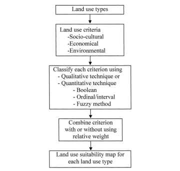
Figure 2.1 A general framework for land use suitability assessment ... 25
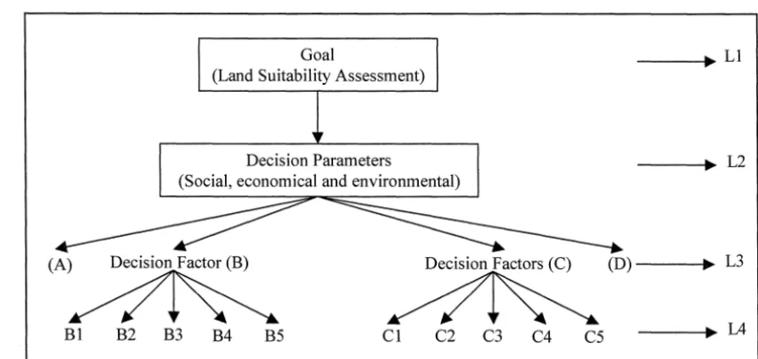
Figure 2.2 Decision hierarchy for AHP process ... 28
Figure 2.3 Membership function for single ideal point ... 33
Figure 2.4 Membership function for multiple ideal points ... 34
Figure 2.5 Membership function for assymetric left (a) and right (b) models ... 34
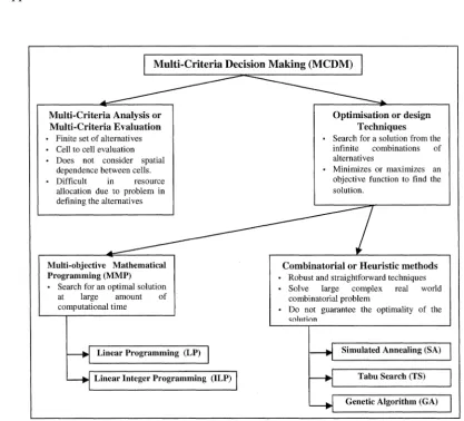
Figure 2.6 Multi criteria decision making approaches in land use decision-making ... 37
Figure 4.1 Research framework for comparing three different methods for solving a MOLAAproblem ... 71
Figure 4.2 Location of the Kioloa Region on the map of Australia ... 74
Figure 4.3 Vegetation map of the Kioloa region···'.··· 77
Figure 4.4 A digital elevation model of the Kioloa region ... 78
Figure 4.5 A geological dataset of the Kioloa Region ... 79
Figure 5.1 Decision framework for a hypothetical MOLAA ... 82
Figure 5.2 Ordinal cost suitability models for different land uses ... 94
Figure 5.3 Continuous cost suitability models for different land uses ... 95
Figure 5.4 Fuzzy cost suitability models for different land uses ... 96
Figure 5.5 Cheapest initial input solution for the large grid of continuous cost model 98 Figure 5.6 Greatest difference initial input solution for the large grid of fuzzy (cost suitability) model ... 99
Figure 6.1 Land use allocation for the Kioloa region by MOLA using ordinal land use suitability model ... 111
Figure 6.2 Land use suitability maps with values for four land uses in the small grid. Black squares indicate NODATA values ... 113
Figure 6.3 Rank maps with values for four land uses in the small grid ... 113
Figure 6.4 Land use allocation for the small grid of ordinal land use suitability model ... 114
Figure 6.5 Land use allocation by MOLA for the continuous land use model ... 114
Figure 7 .1 Comparison of cost functions at very slow cooling rates in Mode 1 with Mode 2 ... 122
Figure 7.2 Comparison of cost functions at very slow cooling rates in Mode 1 with Mode 3 ... 122
Figure 7.3 Improvement in the cost function at different cooling rates ... 124
Figure 7.4 Accepted number of cold-swap at different cooling rates ... 125
Figure 7.5 Accepted number of hot-swaps at different cooling rates ... 125
Figure 7. 7 Cost function minimization by four different swapping rates at very fast cooling rate and high value of initial control parameter. ... 127
Figure 7 .8 Random input solutions and near-optimal land use allocation by Simulated Annealing for the large, medium and small grids using the ordinal cost model ... 130
Figure 7.9 Average computation time at very slow cooling rate and four swapping rates for all three cost models in the medium grid ... 132
Figure 7 .10 Improvement in the spatial compactness applying different compactness factors to the ordinal model for the medium grid MOLAA problem ... 137
Figure 8.1 Run time for the static and dynamic modes at two Tahu lengths for the medium gird ... 149
Figure 8.2 Mean cost functions at eight different Tahu lengths for medium grid (random input solution) of ordinal cost model in static mode ... 151
Figure 8.3 Mean cost function at different swapping rates for medium grid (random input model) of ordinal cost model in static mode ... 152
Figure 8.4 Number of cold-swaps at different swapping rates for the medium grid .... 153
Figure 8.5 Number of hot-swaps at different swapping rates for the medium grid ... 153
Figure 8.6 Improvement in the cost function at different swapping rates with Tahu
length T1 = 48 for the medium grid ... 153
Figure 8.7 Near-optimal land use allocation in the small, medium and large MOLAA problems by Tahu Search using random initial input solution of the ordinal cost suitability model ... 156
Figure 8.8 Computation time for four Tahu lengths at different swapping rates for the large grid in ordinal cost model.. ... 158
Figure 9.1 Comparing the acceptance of hot-swaps and cold-swaps using the
appropriate parameters between the Simulated Annealing and Tahu Search ... 171
Figure 9 .2 Comparing the cost functions using the appropriate parameters between the Simulated Annealing and Tahu Search ... 171
Figure 9.3 Comparing the cost functions minimization by the cold-swaps only between the Simulated Annealing and Tahu Search ... 171
Figure 9.4 Comparing the acceptance of the cold-swaps per step after the hot-swaps became zero in the Simulated Annealing and Tahu Search ... 172
Figure 9 .5 Spatial compactness by three methods in the ordinal model ... 172
Chapter 1
INTRODUCTION
1.1 Research problem
Land use is ever-changing in order to cope with the demands of population growth
(Fisher et al., 1996; Pieri, 1997; Theobald et al., 2000; Ligtenberg et al., 2001). A
global estimate of land use change suggests that 1.2 billion ha. of forest/woodland have
been lost since the 1700s. However, the area of agricultural land expanded by the same
amount in the period (Richards, 1990). Inappropriate land use changes have been
blamed for massive land degradation and associated environmental and social problems
Rossiter, 1996; Nehme and Simoes, 1999). These problems are more pronounced in downstream ecosystems of catchments (Allan et al., 1997) because they affect water
quality, biodiversity and loss of habitat (Dumanski, 1997). In Australia, land
degradation has become the largest environmental problem, causing dry land salinity,
acidification, contamination and vegetation degradation (ASEC, 2001). The cost of this
is estimated to be about A$ 788 millions a year (Castles, 1992). The UN has recognized
land degradation as a global problem affecting the goal of sustainable development and
has been emphasizing the need for action at both local and national levels (WCED,
1987). To arrest further land degradation and environmental problems, the sustainable
use of land resources to the extent of their potential, and not exceeding their capacity,
has become a primary focus within the concept of sustainable development (van Lier,
1998).
Land use planning at the local level has emerged as a primary tool to deal with the
global problem of land degradation; it partially contributes to the achievement of
sustainable development through protecting natural and man-made heritage (Bruff and
Wood, 2000). A major issue in sustainable use of land resources is allocation of the
resources to compatible land uses with respect to land quality and the desire of the
stakeholders concerned. The best possible use of land resources has become imperative
in order to keep a balance between the finite limitations of land resources and the
To this end, a zoning approach has been used in land use planning to control land use but in practice, this approach has failed to cope with the new demands of land use change (Yewlett, 2001). Several methodologies have been developed to assist in the process of land use decision-making for appropriate allocation of desired land uses. This research aims to deal with some of the methodologies of land allocation for sustainable land use planning in order to ensure perpetual benefits to future generations.
Growing concern about the environment and natural resources has given sustainable use of land resource an importance in the public eye. The public is now playing an important role in sustainable land use planning, taking part in and contributing to decision-making processes. In Australia, land use planning is the primary strategy adopted to combat land degradation and other environmental problems, with the involvement of the local communities. The wide public concern over land issues is shown in the establishment of over 4,250 Landcare Groups throughout Australia to work together towards a more sustainable use of the resources (DAFF, 2004). However, land use decision-making about the allocation of available and often limited land resources for meeting social, economic and environmental objectives has become a complex issue in land use planning processes. Ultimately, the land use decision determines the social, economic and environmental conditions in a locality (Arnold, 1999).
Decisions for allocating land use are taken at various spatial scales (Bouma, 2001) by considering bio-physical, social, economic and environmental factors (Fisher et al., 1996). The bio-physical attributes of the land largely determine land quality or suitability for different land uses (Ligtenberg et al., 2001). However, the decisions are mainly subjected to the public (stakeholders) interest and government land use policies. It has become essential to involve the public/stakeholders in land use planning (Selman, 2001). They raise land use issues and set the objectives, the desired land uses and area requirement for each land use type.
1991) or a research and development facility location (Tomlin and Johnston, 1988) are typical examples of a single land use decision problem. However, land use planning at landscape or regional level generally involves several land uses for achieving the wide range of land use objectives desired by the stakeholders. In this situation, land use allocation becomes a multiple land use decision problem. These multiple land uses often compete for the same land unit (Lockwood et al., 1996) and conflicts among land uses become evident. This adds complexity to the land use decision-making, as the conflicting land use needs cannot be met simultaneously under limited resource conditions (Monarchi et al., 1976).
The allocation of multiple and/or conflicting land uses poses a great challenge to decision-makers and planners to arrive at a consensus decision among all the stakeholders. A land use decision to allocate multiple and conflicting land uses requires reconciliation of any conflict by making a trade-off between these land uses based on their relative suitability in order to allocate the best possible land use option to each land parcel. Therefore, a solution to multiple and conflicting land use problems involves the consecutive tasks of suitability assessment of each land unit against each land use alternative and then allocating the most suitable alternative. Such a problem is appropriately described as Multi Objective Land use Assessment and Allocation (MOLAA). This problem is also known by other names such as Multi Objective Land Allocation (Eastman et al., 1993), and Multi site Land Use Allocation (MLUA) (Diamond and Wright, 1989; Aerts, 2002; Aerts and Heuvelink, 2002).
Conflicts of interest among stakeholders are also inevitable in resource allocation decision-making (Bojorquez-Tapia et al., 1994; Lahdelma et al., 2000; Fraser and Chisholm, 2000; Liu and Stewart, 2004; Christou et al., 2004; Wester-Herber, 2004). In addition to such conflicts, the large number of land parcels or units, their spatial variability, the existence of several criteria for land evaluation and also the specified constraints such as area and shape requirements make this problem quite complex and are difficult to solve manually (Tomlin and Johnston, 1988). Therefore, adopting a comprehensive approach for land use planning that integrates social, economic and environmental factors has been emphasized for maintaining the integrity of the social and natural environments and keeping a balance with economic growth (Pieri, 1997; van Lier, 1998). Various techniques and approaches have been developed for land use suitability in order to accommodate diverse groups of stakeholders and take into account their interests in the decision-making. It is believed that these techniques are helpful for reconciling the land use conflict among the stakeholders and achieving a consensus in the multi-objective land use decision-making (Bojorquez-Tapia et al., 2001).
s.
N.
1.
2.
3.
4.
5.
6.
8.
Table 1.1 MCDM techniques for solving single/multiple land use allocation problems
Name of the technique Application and limitation Authors Multi-criteria Group Evaluates feasible land use (Malczewski, Decision-making Model pattern using multiple criteria 1996)
(AHP and Integer Linear Programming)
GIS based multivariate Land use suitability assessment (Bojorquez-application and participatory decision- Tapia et al.,
making 2001)
MAGISTER (Multi-criteria Generates a suitability map for (Joerin and Analysis with GIS for a single land use using Musy, 2000)
Territory) multiple criteria
MCEandGIS Application to agricultural land (Janssen and
use Rietveld, 1990)
Integration of MCE and For single land use allocation (Carver, 1991)
GIS basedonMCE
Multi-objective For single land use allocation (Diamond and
Programming Modelling Wright, 1989)
Integer Linear Multiple land use allocation (Aerts, 2002) Programming for small number of land units
An optimum solution to a MOLAA problem may be achieved by allocating each land parcel (unit) with the best possible land use, meeting all specified constraints (area or shape requirement). The solution will maximize overall land use suitability. However, the optimum solution lies within the innumerable possible combinations of the land units and land use alternatives and constraints (Diamond and Wright, 1989). Computationally, it is not feasible to search for every possible combination of decision variables (land unit and land uses) and constraints (area or shape requirement) to find the optimum solution in a reasonable amount of time, using either systematic or mathematical optimisation techniques within the MCDM. Many real world problems are of this nature and have been classified as combinatorial problems (van Laarhoven and Aarts, 1987; Aarts and Korst, 1989; Voudouris, 1997).
Three famous approximation optimisation techniques that have proven useful for generating an acceptable solution to many real world combinatorial problems are Simulated Annealing, Genetic Algorithm and Tahu Search (van Laarhoven and Aarts, 1987). Simulated Annealing has been successfully applied in solving a multi-objective land use allocation problem in a post-mining restoration site in As Pontes, Spain using raster data (Aerts, 2002). The algorithm delivered a solution by minimizing the cost function, allocating each land unit with the best possible land use, that is, with the lowest development cost. The development cost model was derived by using two land attributes applying different factors for these land uses (Aerts, 2002; Aerts and Heuvelink, 2002). Nevertheless, this algorithm has not been compared with other combinatorial methods so far. Therefore, the comparative performance of Simulated Annealing and the quality of the solution are untested. From an application viewpoint, a comparison of Simulated Annealing with one of the combinatorial methods in solving the same MOLAA problem may provide users with an informed choice of these methods, based on the quality of the solution and the performance of the algorithm.
Although Genetic Algorithms have been used for MOLAA problems at the farm level, they have not been applied at larger scales, that is, landscape or regional scale. Matthews et al. (2000) noted that use of raster data causes computational inefficiency of the algorithm. Tahu Search is not yet tested for a MOLAA problem; however, it has successfully delivered an efficient and effective solution to similar combinatorial problems. Based on its simplicity and on its demonstrated applicability to similar problems using raster data, Tahu Search algorithm has been found to be appropriate for solving the same MO LAA problem in this research in order to compare its solution with that of Simulated Annealing.
The main goal of this study is to compare the performance of two combinatory methods, that is, Simulated Annealing and Tabu Search and the MOLA module in IDRIS!® in order to provide an informed choice among these methods in solving a multi-objective land use allocation problem. In the research design, it was planned to test the application of both combinatory methods in a hypothetical MOLAA problem in the Kioloa region in New South Wales (Australia). The performance of these methods were assessed based on the improvement in the cost function, spatial compactness, computation time and input model requirements.
In land use allocation, a larger patch of the same land use is more desirable for many reasons than a scattered distribution of one land use (Aerts, 2002). For example, a spatially compact reserve area is preferred because of low management cost (McDonell et al., 2002). Hence, a compactness function has been incorporated in both
combinatorial methods to enhance the spatial compactness in land use allocation. The solutions found by applying compactness function were compared between these two methods.
1.2 Research objectives
The main objective of the research is to compare the performance of Simulated Annealing, Tabu Search and the MOLA module in IDRIS!® by applying them to solve a Multi Objective Land use Assessment and Allocation (MOLAA) problem. The aim is to provide an informed choice among these methods to the users. These methods treat each cell of the raster dataset as a land unit and yield a solution by searching for the best possible combination of all the decision variables (land use types and land units). The following parameters will be assessed in the output solution for comparing the performance of these methods:
• improvement (minimization) of the cost functions;
• spatial compactness in terms of number of patches for the different land uses; • enhancement of spatial compactness after incorporating compactness function in
Simulated Annealing and Tabu Search algorithms. • computational (run) time taken to deliver the solution;
are applied with different combination of settings of parameters to three different initial
input solutions derived from three cost suitability models.
1.3 Implications of the research
Land use planners or decision makers facing multiple land use allocation problems during the land use planning process may use these methods as a decision support tool
for generating a solution to a specific MOLAA problem. The selection of one decision
support tool is not an easy task and the users should employ a conscious logic in making
their choice (Lahdelma et al., 2000).
The users would ideally be interested in obtaining the most comprehensive solution, in
the least computational time, with simple data input. However, the solutions generated
by these methods may not be the same. To be able to decide on the most appropriate
method, the users (decision makers/planners) should know have some knowledge of the
methods applicable to the MOLAA problem, as well as the input requirements and the quality of the solutions reached from these methods. This research aims to address these
multiple interests of users; thus, the implications of the research can be broadly stated as
follows.
• To allow the characterization of three methods for different circumstances, data
and intentions;
• To provide users of the MOLAA with information necessary to make informed
choices among these methods.
Decision support tools have been developed to facilitate decision-making by providing
alternative solutions to a problem. However, how good is that solution? The
stakeholders may judge the quality of the solution by assessing whether or not their
values/interests have been truly reflected in the solution. The equity or fairness of the
decision-making process will enhance the effectiveness and acceptability of the decision
(Hunt and Haider, 2001 ). It is necessary for the decision makers to ensure 'procedural fairness' of the decision support tool in order to bring them to a consensus decision.
Hence the implication of this research will also on the 'procedural fairness' of these
i
i
1.4 Background concepts
1.4.1 Land and land use
'Land' has a very wide meaning and scope in geo-political, socio-cultural and economic terms (Hamblin, 2001). Hence, land cannot be defined in an easy way. However, every human can conceive of it in its physical identity. In economic terms, it is the wealth and capital input for production activities. In a geo-technical context, land is the outer crust of the earth and also includes inland water bodies, estuaries and coastal areas. It has a permanent ge9graphical location covering a finite area and can be described by its physical characteristics such as topography, soil and subsurface structure and composition (Davis, 1976). These characteristics are used for classifying land categories and are also taken into account for land use planning.
'Land use' is defined as all kinds of human intervention in order to derive goods and services from land and can be categorized into three groups, production (agriculture, forestry, grazing, mining), services (conservation or ecological services, water production, recreational) and infrastructure development (housing, roads, bridges) (Vink, 1975). According to Eastman et al. (1993) land uses can be both complementary and conflicting. Complementary land uses can co-exist together spatially as well as temporally whereas conflicting land uses cannot.
There have been attempts to classify land uses into coherent groups by generalizing detailed observations. Some of the major land use classifications include the World Land Use Survey (early 1930s), Second Land Utilization Survey (late 1960s), The United States Geological Survey and The National Land Use Classification (Rhind and Hudson, 1980). These broad schemes have attempted to provide land use classification for a particular purpose, and vary widely in terms of the extensiveness of the area, the map scales or source of data (for example remote sensing imagery). None of these classifications coincide in terms of the number of land use classes and their description. In Australia, land uses have most recently been classified into nine classes based on the major use of land and the level of anthropogenic intervention (Stewart, 2001 ).
land use might also be conservation reserve. This research focuses on land use allocation for different uses of land as determined by human beings.
1.4.2 Land valuation and land evaluation
'Land valuation' is the economic gain from the goods and services supported by the land (Davis, 1976; Hanink and Cromley, 1998). Some values attached to land like recreational, environmental, aesthetic and social values are difficult to measure in monetary terms. However, the pricing of these values can be accomplished by some indirect methods like hedonic valuation, travel cost and household production function (Mcconnel, 1993) and contingent valuation (Lockwood et al., 1996).
'Land evaluation' is the quantitative or qualitative assessment process for assessing potential use of land by using some land attributes (Rossiter, 1996). According to the F AO, land evaluation is a part of the land use planning process used to assess the performance of land in terms of economic gain, social impacts and environmental consequences of present land use (F AO, 1976). F AO has developed a Land Evaluation Framework or FAO Framework in order to standardize the methods and reconcile different methods used by different countries (Davidson, 1992). The main aim of land evaluation is to grade land for particular land uses, analysing the social, economic and environmental implications and finally to identify the suitability of the· land for one or more land uses.
1.4.3 Land capability and land suitability
The terms 'land capability' and 'land suitability' seem to be quite similar and are often used interchangeably. Vink (1975) defined these terms as the ability of the land to offer a certain specified land use as determined by the socio-cultural and economic conditions. Davis (1976) has defined land capability in two domains. First, he defined land capability in terms of land itself, as a measure of a combination of inherent physical attributes of the land, the climate and the vegetation. Second, he attempted to classify land capability based on specific land uses such as agriculture, forestry and engineering through assessing the extent of physical limitations, management and conservation requirements. This definition combines both the land's physical characteristics and climatic information and also accounts for the limitations imposed by these physical attributes.
The initial intention was to classify land into different capability classes for agricultural land use. The US Soil Conservation Service had first classified land capability into eight capability classes, four sub-classes and several units based on soil survey data (Rhind and Hudson, 1980). Though this land capability classification was intended to be used in making agricultural decisions, it was applied to all planning purposes (Steiner, 1983). Subsequently, other countries like Canada and Britain developed their own land capability classification, in order to suit land use planning and management (Davidson, 1992). The main aim of these classifications was to facilitate land use planning through categorizing land into different classes or subclasses based on land characteristics, considering the factors and the constraints that favour or limit a land use type.
However, land use decisions based merely on the land's physical attributes were soon realized to be inadequate to satisfy the growing environmental consciousness and economic thinking of the public on land use issues (Bojorquez-Tapia et al., 1994). Planners or decision makers responded to it by including social, economic and environmental implications of proposed land uses besides the land's physical capability. A comprehensive evaluation of land units for particular land uses has thus become essential for assessing their relative suitability for different land uses.
fitness of a land unit for a particular land use. McHarg (1969) used land suitability as
the presence of all the favourable parameters in the absence of the constraints for a
particular land use, making the land 'intrinsically suitable' for that particular use.
Land suitability measures the condition or state of land relative to a particular land use
indicating land quality (Dumanski, 1997). Land quality signifies the condition of land
resources relative to different land uses like agricultwe ~ conservation and forestry (Pieri et al., 1995). It is measured by the suitability of the laind for a specific use and can be
enhanced or degraded by land use type and management practices (Dumanski, 1997). A
land suitability assessment provides a rating for each land unit with respect to its
suitability for each land use, to enable the planners to make an objective decision based on the relative suitability values of all potential land uses; suitability has been
categorized into actual or current suitability and potential land suitability (Brinkman and Smyth, 1973; Vink, 1975; Hall et al., 1992). Current or actual land suitability implies
suitability of land in its present condition, that is, ~thout improving or changing the
land conditions. Potential land suitability takes into account land suitability that is
feasible only after some major land improvement requiring a major capital investment has taken place.
Different approaches have been adopted for analysing land suitability for the purpose of
land use planning. The Dutch method is a land capability classification focused solely
on soil characteristics, thus its approach is mainly appropriate for land suitability
assessment for arable and grassland uses. McHarg (I ~69) proposed a method for land suitability assessment combining the characteristics
of
land use, natural parameters and their compatibility. Within agricultural land use, the la.lid's suitability for different cropshas been extensively researched to aid decision-makiag by providing the best crop type
for each land unit (Johnson et al., 1994; Ahamed et al., 2000; Ceballos-Silva and
Lopez-Blanco, 2003).
This research therefore assesses the relative suitability- of each land unit for all potential
land uses, taking into consideration not only the land's attributes in relation to each land
use type, but also including appropriate spatial or non-spatial, social, economic and
environmental parameters. The inclusion of other evi:tluation criteria besides the land's attributes implies the suitability of the land unit for the prescribed land use rather than
for this research. These evaluation criteria are combined following a rule of combination as decided by the decision makers and the stakeholders. This research applies different approaches to land suitability assessment and the solutions will be compared. The details of these approaches will be discussed in Chapters 2 and 5.
1.4.4 Land use objectives and conflict
Land serves a wide range of objectives that may be social, cultural, economic or environmental. These objectives are the key to making decisions on the evaluation criteria (Huddleston, 2002) and also land use types for ultimate land use allocation for either single or multiple land use types. In the case of a single land use, a decision-making problem may arise when there are several land parcels or units suitable for the specified land use and only one site has to be chosen. It requires an assessment of all potential land parcels and finding the best, most suitable site for the desired land use. This problem has been called a 'single facility location problem' or 'facility siting problem' (Tomlin and Johnston, 1988; Carver, 1991).
A 'Multiple Land Use problem' requires the allocation of the most suitable sites for each land use. However, the multiple land uses must be further segregated into compatible or non-compatible land uses depending on whether they can coexist or not (Eastman et al., 1993). Compatible land uses can be allocated to the same land parcel at the same time. These may be complementary or coexisting land uses. During the designing of the land use problem, compatible land uses can be merged together into one land use type and allocated to the same unit of land.
system for a consensus decision among stakeholders on a multiple and conflicting land use allocation problem.
1.4.5 Land use planning and land use allocation
FAO (1976) defined land use planning as a procedure to identify the most suitable land use from the available land use options, taking into consideration the social and economic conditions and land and water capabilities. However, the involvement of interest groups or stakeholders in land use planning is not made explicit in this definition. Recently, the Sahtu Land Use Planning Board," Canada (2003) defined land use planning as identifying guiding principles for using land and its resources for the social, cultural and economic interests of all the stakeholders. In the Northern Territory Government's (2003: 1) point of view, "land use planning is the process whereby the Government works with the community to establish agreements on how land suitable for development can be identified, serviced, built upon and used for social economic purposes in environmentally sustainable ways".
One of the main goals of land use planning is to achieve economic efficiency, social equity and sustainability of the resource. It is necessary for land use planning to guide decision-making on land use (F AO, 1976). It aims to harmonize economic development with environmental sustainability to fulfil the social, cultural and economic aspirations of the people. Land use planning has become an indispensable part of sustainable development throughout the world to ensure that current as well as future, land use changes will not threaten or damage the environmental· sustainability of the region.
' !
1.5 Organization of the thesis
This thesis focuses on two combinatory methods and one GIS based MOLA module in solving a MOLAA problem and compares their performance in order to provide an informed choice among these methods based on the run time, optimum result and the input required from prospective users (planners or decision makers). The thesis is divided into ten chapters. A brief description of each chapter is presented here:
Chapter 1 : Introduction
This chapter discusses the issues and problems of land use planning/decision-making and formulates a research problem for comparing two combinatory methods and a GIS based MOLA module in IDRISI® software in solving a MOLAA problem. This chapter also presents the research objective, implications and some background concepts in order to clarify relevant terminology in the context of this research.
Chapter 2: Approaches of multi-objective land use decision-making
A framework in the context of land use decision-making is presented in this chapter. Different techniques of land suitability assessment and decision support tools focussing on various methods of the Multi-Criteria Decision Making (MCDM) are discussed based on the available literature.
Chapter 3: Methods for multi-objective land use allocation
The theoretical principles of combinatory methods and Simulated Annealing and Tahu Search algorithm are elucidated here. This chapter also describes the MOLA module in IDRIS!®.
Chapter 4: Research framework and study site
The framework for this research and a brief note on each step in the framework are provided in this chapter. The study site and the available digital datasets are also discussed.
Chapter 5: Methodology
methods. This chapter also specifies the parameters for Simulated Annealing and Tahu
Search.
Chapter 6: Result I - Applying MOLA in solving a hypothetical MO LAA problem
This chapter presents the results obtained after applying the MOLA module in solving a
hypothetical MOLAA problem in the Kioloa region, NSW. The ordinal and continuous
land use suitability models are used and the results are analysed in the MOLAA
problem in a small grid.
Chapter 7: Result II - Applying Simulated Annealing to the hypothetical MOLAA
problem
The results of applying Simulated Annealing to the hypothetical MOLAA problem
using the ordinal, continuous and fuzzy cost suitability models are presented. Different
combinations of annealing schedules are applied to three different initial input solutions
produced by the random, cheapest and greatest difference methods. An appropriate
annealing schedule and initial input model will be sought for applying Simulated Annealing to a MO LAA problem.
Chapter 8: Result III -Applying Tahu Search to the hypothetical MOLAA problem
This chapter presents the results of applying Tahu Search to the same hypothetical
MOLAA problem using the same cost suitability models. Different parameters and
initial input solutions are used for finding the best parameter combinations and input
solution for applying Tahu Search to a MO LAA problem.
Chapter 9: Result IV - Comparing the combinatory methods and MOLA module in
solving the hypothetical MOLAA problem
The solutions obtained by applying Simulated Annealing, Tahu Search and the MOLA
module to the same hypothetical MOLAA problem are compared in this chapter. The
quality of the solution and efficiency of these methods are compared and assessed in
solving a MO LAA problem.
Chapter 10: Conclusions
This chapter presents the conclusions reached in relation to this research. The conclusions are drawn on the appropriateness of application of each of these methods in
solving a MOLAA problem using the different input rriodels chosen. Recommendations
1.6 Papers from this thesis
Sharma S. K. and Lees B. G., 2004 A comparison of simulated annealing and GIS
-I
based MOLA for solving Multi-Objective Land use Assessment and Allocation Problem. Paper presented at XVII International Conference on Multi-Criteria Decision Making,
6-11 Aug. 2004, Whistler, British Colombia, Canada.
Sharma, S. K., 2004 Spatial decision support using Simulated Annealing, Paper presented at the Fifth Australasian Postgraduate Workshop on GISc, Social and
Environmental Modelling, 1-6 Feb. 2004, Kioloa, New South Wales, Australia.
Chapter 2
APPROACHES TO MULTI-OBJECTIVE LAND USE
DECISION-MAKING
2.1 Introduction
Multi-Objective Land use Assessment and Allocation (MOLAA) is a typical example of
a land use decision-making problem. In this problem, the prime aim of the decision
maker is to reach a consensus decision on land use allocation among stakeholders
through maximizing the overall land use suitability of multiple and often conflicting
land uses. In order to approach a MOLAA problem at landscape or regional scale, it is
imperative for the decision makers to follow a framework of land use decision-making which enables them to achieve the above aim. This chapter will briefly explain the
concept of decision-making in the context of land use, present an analytical framework
and describe each element of the framework. Various approaches and techniques have
also been developed to deal with the complexity of land use decision-making. This
chapter will thus also evaluate some of these approaches and techniques being used for
land use decision-making.
2.2 Land use decision-making
Decision-making is a situation that arises due to the availability of choices or options to
address a problem. Hwang et al. (1979) defined decision-making as a process of
choosing appropriate option(s) to accomplish desired objective(s) from the potential
alternatives. To Eastman et al. (1993), it is a selection from a set of available options,
actions or expectations. He called these alternatives the "decision frame" and referred to
the area where the decision frame is applied as the "candidate set". The set belonging to
each member of a decision frame is called a "decision set". In decision-making one has to decide which decision frame applies to each of the candidate sets. The above
definitions by Hwang et al. (1979) and Eastman et al. (1993) imply that land use
decision-making is a process of matching available land parcels with appropriate land
Land use decision making with several stakeholders or decision makers has become a very complex task because of conflicts of interest regarding the land use (Mills and Clark, 2001). This difficulty may be attributed to differences in socio-economic aims among the stakeholders (Bojorquez-Tapia et al., 2001). Land itself adds complexity to the decision-making process, as not all land is suitable for all land uses, rather it offers varying relative suitability for different land uses, depending upon the land's characteristics together with the land use requirement (Hall et al., 1992). A land unit may be suitable for more than one non-compatible land use, all of which could not co-exist on the same land unit in the same time and space (Eastman et al., 1993). In addition, the immobility and finiteness of the land add further limitations to the land use decision-making process.
Land use decision-making for a single land use is relatively easy and straightforward and can be accomplished by comparing the suitability values of the entire available, potential land parcels. However, the decisions become more complex and challenging with the involvement of multiple land uses due to the involvement of stakeholders having social, economic and political differences (Brill et al., 1982). Davis (1976) has ascribed the complexity of land use decision-making to divided land ownership, and multiple authorities among the federal and state governments, private landowners and interest groups. However, the severity of the problem may be attributed to the sensitivity of the area, its social, economic and environmental importance and the extent of the area. At farm level, land use decisions have been found to be influenced by the land holding size and also the economic status of the farmer (Ravnborg and Rubiano, 2001). As in other domains, land use decision-making is also characterized by risk and uncertainty due to the incompleteness and lack of accuracy of the datasets (Aerts, 2002). In summary, land use decision-making problems tend to be case-specific and are governed by the extent (size), data sources and their accuracy, heterogeneity among the stakeholders and their land use interests and also the bio-physical characteristics of the land itself.