Performance Improvement Of Split Savonius Rotor By CFD

(1)

PERFORMANCE IMPROVEMENT OF SPLIT SAVONIUS ROTOR BY CFD

NUR HAYATI BINTI HASSAN

(2)

PERFORMANCE IMPROVEMENT OF SPLIT SAVONIUS ROTOR BY CFD

NUR HAYATI BINTI HASSAN

This report is submitted

in fulfillment of the requirement for the degree of Bachelor of Mechanical Engineering (Thermal-Fluids)

Faculty of Mechanical Engineering

UNIVERSITI TEKNIKAL MALAYSIA MELAKA

(3)

ii

DECLARATION

I declare that this project report entitled Performance Improvement of Split Savonius Rotor by CFD is the result of my own work except as cited in references.

(4)

iii APPROVAL

I hereby declare that I have read this project report and in my opinion this report is sufficient in terms of scope and quality for the award of Bachelor of Mechanical

Engineering (Thermal-Fluids)

(5)

iv

DEDICATION

(6)

v ABSTRACT

(7)

vi ABSTRAK

Turbin angin Split Savonius adalah sejenis turbin angin vertikal. Turbin angin Split

Savonius yang asas terdiri daripada dua jenis bilah iaitu bilah mara dan bilah kembali.

Bilah mara menghasilkan daya seret dari aliran utama manakala bilah kembali

menghasilkan daya kembali dari arah bertentangan melalui jurang yang dikenali sebagai

pertindihan. Dua jenis daya kilas dijana daripada pergerakan putaran antara bilah-bilah

ini dan bendalir yang digunakan iaitu daya kilas positif dan negatif. Objektif utama kajian

ini adalah untuk mengendalikan analisa numerik dua dimensi antara pemutar asas Split

Savonius dan konfigurasi baru dari segi daya kilas positif bersih dan pekali prestasi. Tiga

jenis konfigurasi baru direka berdasarkan pemutar asas Split Savonius dengan

mengekalkan diameter plat, pertindihan dan nisbah aspek malar. Kajian pensahihan

dilaksanakan dengan membandingkan nilai daya kilas yang diperolehi daripada kaedah

numerik dengan nilai daya kilas yang diperolehi daripada kaedah eksperimentasi.

Metodologi yang sahih tersebut digunakan bagi mensimulasi konfigurasi baru.

Peningkatan pekali prestasi antara nilai 0.78% sehingga 1.33% telah dicapai bagi halaju

masuk yang berbeza-beza untuk konfigurasi 1. Konfigurasi-konfigurasi lain tidak

(8)

vii

ACKNOWLEDGEMENT

Alhamdulillah. I would like to express my greatest appreciation towards my supervisor, Dr. Cheng See Yuan who I would not be able to complete this study without. Thank you for accepting me as your PSM’s student and giving me the opportunity to learn so much from you. Thank you for constantly advising and guiding me throughout this study with patience.

I would like to thank other FKM lecturers for sharing their knowledge in respective area of study. I would also like to thank UTeM’s CAE assistant engineer, Mr. Rizal for allowing me to use the facility and ensuring it is in the best condition.

(9)

viii CONTENT

CHAPTER CONTENT PAGE

DECLARATION ... ii

APPROVAL ... iii

DEDICATION ... iv

ABSTRACT ... v

ABSTRAK ... vi

ACKNOWLEDGEMENT ... vii

LIST OF FIGURES ... x

LIST OF TABLES ... xiii

LIST OF ABBREVIATIONS ... xiv

LIST OF SYMBOLS ... xv

INTRODUCTION ... 1

1.1 BACKGROUND ... 1

1.2 PROBLEM STATEMENT ... 3

1.3 OBJECTIVE ... 4

1.4 SCOPE OF PROJECT ... 4

LITERATURE REVIEW ... 5

2.1 ENERGY IN THE WIND ... 5

2.2 WIND TURBINE ... 6

2.3 OPTIMIZATION OF SAVONIUS WIND TURBINE ... 7

2.3.1 BLADE DESIGN ... 7

2.3.2 NUMBER OF BLADES ... 10

2.3.3 END PLATE DESIGN ... 11

2.3.4 NUMBER OF STAGES ... 12

2.3.5 OVERLAP RATIO ... 12

2.3.6 ASPECT RATIO ... 13

(10)

ix

METHODOLOGY ... 15

3.1 INTRODUCTION ... 15

3.2 GEOMETRY ... 17

3.3 MATHEMATICAL MODELLING ... 21

3.3.1 GOVERNING EQUATION ... 22

3.3.2 TURBULENCE MODELLING ... 23

3.3.3 MESHING ... 25

3.3.4 SETUP AND SOLUTION ... 33

3.3.5 SOLUTION CONVERGENCE 34

RESULTS AND DISCUSSION ... 49

4.1 VALIDATION STUDY ... 49

4.2 COMPARATIVE STUDY ... 50

SUMMARY ... 75

REFERENCES ... 76

(11)

x

LIST OF FIGURES

Figure 1.1 Darrieus Wind Turbine. (Source: McAdam, 2016) 2 Figure 1.2 Conventional Savonius Wind Turbine. (Source: REUK.co.uk, Wenlong Tian,

2015) 2

Figure 1.3 Split Savonius Wind Turbine. (Source: Frederikus Wenehenubuna, Andy Saputraa, Hadi Sutanto, 2014) 3 Figure 2.1 Streamlines, primary and opposing torques. (Source: John Patrick Abraham, 2012) 7

Figure 2.2 40 Degree Twisted Blade. (Source: Abdul Qadir Versiani, 2015) 9 Figure 2.3 3D view of helical Savonius turbine. (Source: A. Reza Hassanzadeh, 2013) 9

Figure 2.4 Rotor configurations. (Source: J., 2007) 10

Figure 2.5 Applied boundary conditions. (Source: Sukanta Roy, 2013) 14

Figure 3.1 Methodology flow chart 16

Figure 3.2 Schematic of two-bladed conventional Split Savonius rotor. (Source: U.K Saha, 2008) 17

Figure 3.3 CAD drawing of computational domain for Conventional Split Savonius wind turbine 18

Figure 3.4 Schematic of Design 1 19

Figure 3.7 Triangular Meshing for Conventional Savonius 25

Figure 3.8 Transition between Stationary and Rotating Domains for Conventional Rotor 26

Figure 3.9 Prism Mesh Layers around Blade in Rotating Domain for Conventional Rotor 26

Figure 3.10 Triangular Meshing for Design 1 27

Figure 3.11 Transition between Stationary and Rotating Domains for Design 1 27

(12)

xi

Figure 3.15 Prism Mesh Layers around Blade in Rotating Domain for Design 2 29

Figure 3.18 Prism Mesh Layers around Blade in Rotating Domain for Design 3 31

Figure 3.19 Mesh Metrics Spectrum. (Source: Ozen Engineering, 2014) 32

Figure 3.20 Monitors for Conventional rotor at V = 6.0 m/s (a) scaled residual (b) moment coefficient (c) drag coefficient (d) lift coefficient 37

Figure 3.23 Monitors for Design l rotor at V = 6.0 m/s (a) scaled residual (b) moment coefficient (c) drag coefficient (d) lift coefficient 40

Figure 3.24 Monitors for Design 1 rotor at V = 8.23 m/s (a) scaled residual (b) moment coefficient (c) drag coefficient (d) lift coefficient 41

(13)

xii

Figure 4.2 Torque per height against inlet velocity for conventional rotor, design 1, design

2 and design 3 52

Figure 4.3 Coefficient of performance against inlet velocity for conventional rotor, design 1, design 2 and design 3 52

Figure 4.4 Variation of torque of conventional rotor with time value for V = 6.0 m/s 54

Figure 4.5 Variation of torque of conventional rotor with time value for V =8.23 m/s 55

Figure 4.6 Variation of torque of conventional rotor with time value for V =10.17 m/s 56

Figure 4.7 Variation of torque of Design 1 rotor with time value for V = 6.0 m/s 57

Figure 4.16 Velocity Distribution for V = 6.0 m/s (a) Conventional (b) Design 1 (c) Design 2 (d) Design 3 67

Figure 4.19 Pressure Distribution for V = 6.0 m/s (a) Conventional (b) Design 1 (c) Design 2 (d) Design 3 70

Figure 4.20 Pressure Distribution for V = 8.23 m/s (a) Conventional (b) Design 1 (c) Design 2 (d) Design 3 71

(14)

xiii

LIST OF TABLES

Table 1 Conventional Split Savonius Dimensions (Source: U.K Saha, 2008) 18

Table 2 Design 1 Dimensions 19

Table 5 Variation of Reynolds Number and Turbulence Intensity. (Source: U.K Saha,

2008) 23

Table 6 Estimated values of turbulent kinetic energy and turbulent dissipation rate.

(Source: U.K Saha, 2008) 24

Table 7 Details of specific dissipation rate and turbulent viscosity ratio. (Source: U.K Saha,

2008) 24

Table 8 Total Number of Elements and Nodes 31

Table 9 Mesh quality metrics 31

(15)

xiv

LIST OF ABBREVIATIONS

BC Before Century

HAWT Horizontal Axis Wind Turbine VAWT Vertical Axis Wind Turbine CFD Computational Fluid Dynamics

CAD Computer Aided Drawing

2D Two Dimensional

3D Three Dimensional

RANS Reynolds Average Navier Stokes

LES Large Eddy Simulation

DNS Direct Numerical Simulation PDE Partial Differential Equation

ASM Algebraic Stress Model

RSM Reynolds Stress Model

TBS Tandem Blade Savonius

TSR Tip Speed Ratio

(16)

xv

LIST OF SYMBOLS

𝐶𝑂𝑃 Power Coefficient/ Coefficient of Performance 𝑃𝑠 Shaft Power/ Mechanical Power

P Power Available in The Wind

T Torque

Ω Angular Velocity/ Rotational Velocity

Ρ Density

A Area

V Velocity/ Speed

𝐷𝑓 Diameter of End Plate

D Diameter of Rotor

D Diameter of Chord

T Thickness of Chord

E Overlap

e’ Second Overlap

N Frequency of Rotation (rpm)

(17)

1 CHAPTER 1

INTRODUCTION

1.1 BACKGROUND

The Sun radiates 1.74×1017_{W energy to the Earth per hour and approximately 2%} of this energy is converted into wind energy (Energy and Environment, 2016). Wind has been used as a source of energy as early as 5000 BC when wind energy is used to propel boats along Nile River (Wind Energy Foundation, 2016). By the end of 2015, 432.9GW wind power capacity has been installed globally led by Germany and United States of America (Global Wind Energy Council, 2016). This improvement has been possible with the use of wind turbine technology. Wind turbine is used to generate electricity by converting kinetic energy of the wind into mechanical energy which is used to turn the rotor and power up the generator, thus, generating electricity.

(18)

2

efficiency due to lack of body force and surface force (Bagus Wahyudi, Sudjito Soeparmanb, H W M Hoeijmakersc, 2014). However, Savonius wind turbine is built due to its uncomplicated and low cost construction (Bagus Wahyudi, Sudjito Soeparmanb, H W M Hoeijmakersc, 2014) (Abdul Qadir Versiani, 2015). It is a slow rotating machine with higher torque compared to Darrieus wind turbine. Savonius rotor is not affected by the direction of wind thus suitable for non-uniform wind areas (Bagus Wahyudi, Sudjito Soeparmanb, H W M Hoeijmakersc, 2014) (Abdul Qadir Versiani, 2015). It is normally used for small water pumping applications.

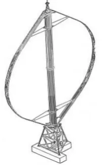
[image:18.595.255.356.259.422.2]

Figure1.1 Darrieus Wind Turbine. (Source: McAdam, 2016)

(19)

[image:19.595.179.437.81.225.2]

3

Figure 1.3 Split Savonius Wind Turbine. (Source: Frederikus Wenehenubuna, Andy Saputraa, Hadi Sutanto, 2014)

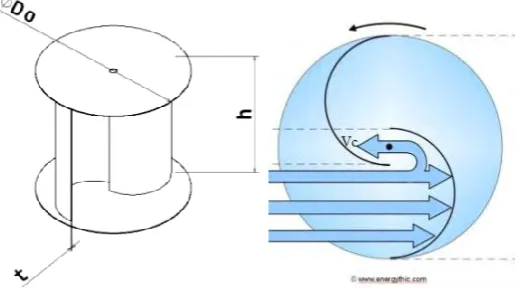
Basic Split Savonius wind turbine consists of two blades; advance blade and return blade. Advance blade produces drag force from main flow whereas return blade develops return force from opposite direction through a gap between blades called overlap. Overlap serves as an entry of outflow from advance blade to return blade. Overlap is the main difference between Conventional Savonius wind turbine and Split Savonius wind turbine (Bagus Wahyudi, Sudjito Soeparmanb, H W M Hoeijmakersc, 2014). There are few modification done to improve Split Savonius rotor in previous researches such as number of blades, blades twist angle, number of stages, overlap ratio, aspect ratio and end plates presence.

1.2 PROBLEM STATEMENT

(20)

4

1.3 OBJECTIVE

The research objective is:

1. To conduct a two dimensional comparative study between conventional Split Savonius rotor and new configured Split Savonius rotors by performing CFD analysis.

1.4 SCOPE OF PROJECT

The scopes of research are:

1. Wind velocities used are 6.0, 8.23, and 10.17 m/s.

2. Modification is made to conventional Split Savonius rotor by changing the rotor shape to obtain higher torque.

3. Three new rotor configurations are drawn by using commercial software, ANSYS DesignModeler.

4. CFD simulation is performed by using commercial CFD software, ANSYS Fluent to study moment coefficient at the blades.

5. Torque and coefficient of performance are calculated by using these values.

(21)

5 CHAPTER 2

LITERATURE REVIEW

2.1 ENERGY IN THE WIND

According to Albert Betz in 1919, any wind turbine regardless the design, is only capable of converting not more than 59.3% of wind kinetic energy into mechanical energy. Betz limit is also known as the theoretical maximum power efficiency of wind turbines. Power efficiency of wind turbine can be measured by using power coefficient equation, 𝐶𝑂𝑃. 𝐶𝑂𝑃 is the ratio between mechanical power and power available in the wind.

𝐶𝑂𝑃 = 𝑃𝑠

𝑃 (2.1)

Where 𝑃𝑠 , is the mechanical power and 𝑃 is the power available in the wind. Mechanical power of wind turbine can be calculated by using equation (2.2).

𝑃_𝑠 = Tω (2.2)

Where T is the mechanical torque (Nm) and ω is the angular speed (rad/s). In the present study, brake torque is considered as mechanical torque for above equation. Angular speed can be calculated from equation (2.3).

ω = 2𝜋𝑁₆₀ (2.3)

(22)

6

Power available in the wind can be calculated by using equation (2.4).

𝑃 = 1₂ρA𝑉3 _(2.4)

Where ρ is the air density (kg/𝑚3_{), A is the projected area of the rotor (}_𝑚2_{) and V is the} wind speed (m/s).

2.2 WIND TURBINE

Bagus wahyudi et al. in his study states that Savonius wind turbine is a pure drag type wind turbine which highly influenced by density, blade sweep area and fluid velocity (Bagus Wahyudi, Sudjito Soeparmanb, H W M Hoeijmakersc, 2014). However, according to Abdullah Al-Faruk et al., it is observed that at low angle of attack, lift force contributes to the overall torque generation which then concluded Savonius wind turbine is a combination of drag and lift forces type of wind turbine (Abdullah Al-Faruk, 2016). As mentioned earlier VAWT has lower efficiency compared to HAWT. Regardless its low efficiency, VAWT is used due to several advantages. VAWT is smaller than HAWT thus requires smaller footprint compared to HAWT. Due to this advantage, some of VAWT application involves other building in which VAWT is mounted to such as cellular communication tower (John Patrick Abraham, 2012). VAWT does not need control system to search for wind direction as it is able to rotate regardless the flow direction. VAWT is able to start rotate at lower wind speed compared to HAWT thus it is suitable to be used for power generation at lower wind speed area. VAWT rotates slower than HAWT resulting in higher mechanical power compared to HAWT.

(23)

[image:23.595.162.448.72.312.2]

7

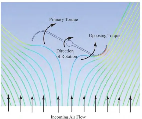
Figure 2.1 Streamlines, primary and opposing torques. (Source: John Patrick Abraham, 2012)

2.3 OPTIMIZATION OF SAVONIUS WIND TURBINE

Number of researches has been conducted to increase the efficiency of Savonius wind turbine. Mohammed Hadi Ali states that performance of Savonius wind turbine is related to these three principles; speed of blade tip is directly proportional to speed of the wind, maximum torque is proportional to the speed of wind squared and maximum power is proportional to the speed of wind cubed (Ali, 2013). Optimization of Savonius wind turbine is measured by using 𝐶𝑂𝑃 equation. Thus, researchers normally compared their new configurations with conventional torque which is then used to calculate 𝐶𝑂𝑃.

2.3.1 BLADE DESIGN

(24)

8

and improve balancing of the couple forces. Previously, three models with different tandem blades configuration were simulated by CFD; Overlap TBS, Symmetrically TBS and Convergent TBS (B Wahyudi, 2013). By using maximum pressure gap between upstream and downstream equation, it is determined that Convergent TBS is capable of generating more power compared to the others. Water is used as working fluid in this study to increase the fluid momentum force acting on the blade. Response surface method and CFD show the variation in velocity and pressure near blades region. Pressure gap occurs across the rotor from upstream to downstream area indicate that power extracted by the rotor is causing it to rotate. Static pressure on convex side of both blades is lower than those on concave side due to high water velocity flowing over the convex side which produce torque to rotate the blades. Drag force acting on the return blade is increased due to compartment gap narrowing in tandem blades adjacent to the axis which increase pressure dynamics on the concave blades. It is observed that with the use of both deflector and tandem blade, velocity ratio on narrow gap and torque produced by drag force on return blade are improved compared to the configuration with tandem blades alone. Deflector caused positive static moment at any tip diameter for both angle deflector designs; radial and tangential whilst configuration without deflector shows the presence of negative values in some range.