This is a repository copy of Spectral Filtering as a Tool for Two-Dimensional Spectroscopy: A Theoretical Model.
White Rose Research Online URL for this paper: http://eprints.whiterose.ac.uk/133173/
Version: Supplemental Material
Article:
Green, D, Camargo, FVA, Heisler, IA et al. (2 more authors) (2018) Spectral Filtering as a Tool for Two-Dimensional Spectroscopy: A Theoretical Model. Journal of Physical
Chemistry A, 122 (30). pp. 6206-6213. ISSN 1089-5639 https://doi.org/10.1021/acs.jpca.8b03339
© 2018 American Chemical Society. This is an author produced version of a paper
published in Journal of Physical Chemistry A. Uploaded in accordance with the publisher's self-archiving policy.
[email protected] https://eprints.whiterose.ac.uk/
Reuse
Items deposited in White Rose Research Online are protected by copyright, with all rights reserved unless indicated otherwise. They may be downloaded and/or printed for private study, or other acts as permitted by national copyright laws. The publisher or other rights holders may allow further reproduction and re-use of the full text version. This is indicated by the licence information on the White Rose Research Online record for the item.
Takedown
If you consider content in White Rose Research Online to be in breach of UK law, please notify us by
Spectral Filtering as a Tool for Two-Dimensional
Spectroscopy: A Theoretical Model
SUPPORT INFORMATION
Dale Green,
†Franco V. A. Camargo,
†,¶Ismael A. Heisler,
†Arend G. Dijkstra,
‡and Garth A. Jones
∗,††School of Chemistry, University of East Anglia, Norwich Research Park, Norwich, NR4
7TJ, UK
‡School of Chemistry, University of Leeds, Leeds, LS2 9JT, UK
¶CAPES Foundation, Ministry of Education of Brazil, Brasilia DF 70040-202, Brazil
This document contains a complete description of the theoretical model used in this study,
in support of the summary presented in the main text. All Liouville pathways involved in
the analysis are presented, as well as further details of the porphyrin monomer modelled and
additional examples of the calculated 2D spectra.
Porphyrin Monomer
In this work we model the same bisalkynyl porphyrin molecule used by Camargo et al in
reference 1, for which the linear absorption spectrum shows three bands, associated with
three accessible excited singlet states. The lowest in energy of these,S1, corresponds to the
Q band, which has a maximum for the fundamental transition at 15 650 cm−1. The second
band, B, (ca. 21000 - 24 000 cm−1) to S
2 is significantly more intense than the Q band and
the third band,N toS3 is very weak, but very broad (ca. 28000 - 34 000 cm−1). Asymmetric
substituents on the porphyrin macrocycle result in a lowering of the molecule’s symmetry
fromD4htoD2h, separating the dipole moment into individualxandycontributions. TheQx band shows a clear vibronic progression due to coupling to a zinc-porphyrin breathing mode
of 375 cm−1. The shallow band at ca. 17 000 cm−1 contains contributions fromQ
y as well as
Qx overtones resulting from coupling to a higher energy vibrational mode of 1340 cm−1.2–4 The structure of the bisalkynyl zinc porphyrin and its linear absorption spectrum are
pre-sented in figure S1, reproduced from reference 1. Here we restrict our model to the vibronic
Qx band and consider coupling to only the 375 cm−1 mode. We assume any contribution from Qy is small because the maximum Qy intensity is less than 30% of the maximum Qx
intensity, causing the vibronic progressions associated with Qy to be similarly weaker, and
Qy to Qx relaxation takes place in 110 fs or less.5 Accounting for energy transfer between modes is beyond the scope of this work, where the inclusion of additional modes rapidly
OC8H17
C8H17O
N N
N N
OC8H17
C8H17O
Si(C6H13)3
(C6H13)3Si Zn
Qx
[image:4.612.96.497.84.227.2]Qy
Figure S1: Molecular structure (left) and linear absorption spectrum (right) of the 5,15-bisalkynyl zinc porphyrin monomer.
Theoretical Model
Vibronic Hamiltonian
The system Hamiltonian is constructed from the ground,|gi, and first excited,|ei, electronic
states,
HS =|gihghg|+|eihehe| (S1)
where intramolecular vibrational modes are introduced in the nuclear Hamiltonians as the
sum of simple harmonic oscillators,6
hg =
X
j
p2
j 2mj
+1 2mjω
2
jq2j
(S2)
he = ¯hωeg0 +
X
j
p2
j 2mj
+ 1 2mjω
2
j(qj −dj)2
(S3)
Here mj, pj and qj are respectively the mass, the momentum and the spatial coordinate of
a particular vibrational mode, j, of frequency ωj. The excited electronic state is raised by
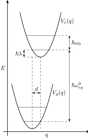
the fundamental transition energy, ¯hω0
eg, and is coupled linearly to the system coordinates
q E
d ~ω
0 eg
~ω0
~λ
Vg(q)
[image:5.612.215.395.73.356.2]Ve(q)
Figure S2: Potential Energy Surface of the displaced harmonic oscillator.
On conversion to a dimensionless coordinate system using,
Pj =
p
¯
hωjmj
−1
pj; Qj =
r
ωjmj ¯
h
qj; ∆j =
r
ωjmj ¯
h
dj
the nuclear Hamiltonians can be written as,
hg = 12
X
j ¯
hωj(Pj2+Q2j) =
X
j ¯
hωj
b†jbj +12
(S4)
he = ¯hωeg0 + 12
X
j ¯
hωj Pj2+ (Qj−∆j)2
= ¯hωeg0 +X j
¯
hωj
b†jbj − ∆j
√
2(bj +b
†
j) + 12∆ 2
j +12
= ¯h(ωeg0 +λ) +X j
¯
hωj
b†jbj− ∆j
√
2(bj+b
†
j) + 12
(S5)
are the vibrational annihilation (creation) operators,
b† =
r
mω
2¯h
q− i mωp
= √1
2(Q−iP) (S6)
b =
r
mω
2¯h
q+ i
mωp
= √1
2(Q+iP) (S7)
such that,
b†b = 1
2(Q−iP)(Q+iP)
Q= b+b
†
√
2 and P =
b−b†
i√2
The reorganisation energy, ¯hλ, is related to the Huang-Rhys parameter, S, by
λ=X j
λj =
X
j
Sjωj =
X
j
mjωj2d2j
2¯h (S8)
Sj = 12∆2j =
mjωjd2j
2¯h (S9)
The system Hamiltonian is then diagonalised to incorporate the off-diagonal coupling
terms and determine the accurate vibronic eigenfunctions. All simulations are completed
using the adiabatic vibronic basis.
Bath Hamiltonian
The environment is defined as an infinite ensemble of harmonic oscillators, such that the
total bath Hamiltonian is given by,
HB =
X
n
X
α
p2
nα 2mnα
+1 2mnαω
2
nαx
2
nα
=X n
X
α ¯
hωnα a†nαanα+12
(S10)
Here, mnα, pnα and ωnα are respectively the mass, the momentum and the frequency of the
The bath modes couple linearly to the system, such that the total interaction Hamiltonian
(including HB) is,
HI =
X
n
X
α
"
p2
nα 2mnα
+ 1 2mnαω
2
nα
xnα−
gnα
mnαω2nα
Bn(q)
2#
(S11)
where gnα is the dimensionless coupling strength and Bn(q) is a system operator which
controls the action of the bath onto the system coordinates, q.7,8
The distribution of coupling strengths is described by the spectral density of each bath,
Jn(ω).
Jn(ω) =
X
α
g2
nα 2mnαωnα
δ(ω−ωnα) (S12)
Every spectral density is assumed to have the Debye form for an overdamped Brownian
oscillator,
Jn(ω) = 2ηn
ωγn
ω2+γ2
n
(S13)
In our model, we separate the environment into three baths to individually account
for dephasing processes (n = 1), intramolecular vibrational relaxation (IVR) (n = 2) and
fluorescence (n = 3). The bath coupling operators are defined as,
B1 = (− |gi hg|+|ei he|)⊗
X
ν
|νihν| (S14)
B2 =|gi(b+b†)hg|+|ei(b+b†)he| (S15)
B3 = ˆµ= (|gihe|+|eihg|)⊗
X
ν
|νihν| (S16)
where P
ν|νihν| is the identity operator over the nuclear degrees of freedom and ˆµ is the dipole moment operator of the system. These operators are then transformed to the adiabatic
vibronic basis using the same unitary transformation with which the system Hamiltonian
was diagonalised.
phonon baths are set to be the same, whilst the coupling strength of the fluorescence bath is
chosen to be very weak (η3 = 1 cm−1). This allows the definition of a complete model, whilst
acknowledging that the fluorescence timescale of the porphyrin monomer is significantly
slower (ca. 1 ns) than the timescale of the photon echo simulations (≤1 ps) in this study.
Hierarchical Equations of Motion (HEOM)
For a bath of harmonic oscillators, the correlation function is related to the spectral density
via,
Cn(t) = 1
π
Z ∞
0
dωJn(ω)
coth
β¯hω
2
cosωt−isinωt
(S17)
where β is the inverse temperature, assumed the same for all baths.
The solution of this integral can be expressed as the sum of exponential terms,9
Cn(t) = ηnγn
" cot ¯ hβγn 2 −i
exp (−γnt) +
∞
X
k=1
8πk
(2πk)2−(¯hβγ
n)2 exp
−2¯hβπkt #
(S18)
which can then be re-expressed in terms of the bosonic Matsubara frequencies, νnk;k =
0,1,2, ..., M, and corresponding exponential prefactors, cnk,6,10
Cn(t) = ηnγn
" cot ¯ hβγn 2 −i
exp (−νn0t) +
M
X
k=1
4νnk ¯
hβ(ν2
nk −γn2)
exp (−νnkt)
#
= M
X
k=0
cnke−νnk|t| (S19)
νn0 = γn (S20)
νnk = 2πk
¯
hβ (S21)
cn0 = ηnγn
cot ¯ hβγn 2 −i (S22)
cnk =
4ηnγn ¯
hβ
νnk
ν2
nk−γn2
The evolution of the density matrix is separated into a hierarchy of auxiliary density
operators (ADOs), ρj, given by
˙
ρj(t) = −
i
¯
hL+
N
X
n=1
M
X
k=0
jnkνnk
!
ρj(t)−i
N
X
n=1
M
X
k=0
Bn×ρj+nk(t)
−i
N
X
n=1
M
X
k=0
jnk
cnkBnρj−
nk(t)−c
∗
nkρj−
nk(t)Bn
−
N
X
n=1
2ηn ¯
hβγn −
ηncot
¯
hβγn 2
−
M
X
k=1
cnk
νnk
!
Bn×Bn×ρj(t) (S24)
where L is the Liouvillian operator and B×
nρ = [Bn, ρ] denotes the commutator of the bath coupling operator, Bn, and the density matrix.11
The ADOs are defined in terms of theN(M+1)-dimensional vectorsj= (j10, . . . , jnk, . . . , jN M) andj± = (j
10, . . . , jnk±1, . . . , jN M), which contain elements for each Matsubara frequency of each bath. The coefficients of the vectors, jnk, define the depth of the hierarchy for a
partic-ular ADO, with the true reduced density matrix equivalent to the ADO with all coefficients
equal to zero.
The hierarchy must therefore be terminated with respect to the number of Matsubara
frequencies involved and the depth associated with each frequency. We adopt the termination
criterion of Dijkstra and Prokhorenko, who select a convergence parameter, Γ, beyond which
the evolution is assumed to be within the Markovian limit.11 The convergence parameter
determines the number of Matsubara frequencies via,
2(M + 1)π
β >Γ (S25)
and the hierarchy depth according to,
N
X
n=1
M
X
k=0
jnkνnk >Γ (S26)
the timescale of the bath fluctuations.
Linear Absorption Spectrum
The linear absorption spectrum is calculated as the Fourier transform of the first order
molecular response function, R(1)(t 1).9,12
σA(ω)∝
Z ∞
−∞
dteiωtR(1)(t1)∝
Z ∞
−∞
dteiωtTrg
ˆ
µGˆ(t1, t0)[ˆµ, ρ(−∞)]
(S27)
Here the trace is taken over the ground state degrees of freedom only and the dynamical
map ˆG(t1, t0) indicates use of the HEOM to propagate the result of the commutator from
time t0 to time t1.
2D Photon Echo Spectroscopy
The pulse sequence for four-wave mixing 2D photon echo spectroscopy is depicted in figure
S3. Whilst τ,T and t define the separation of the pulse centres and the signal, as described
in the main text, the interaction events can occur at any time under the Gaussian envelopes.
Hence the separation of the interaction events is given by t1, t2 and t3, which are the time
references used in the double-sided Feynman diagrams presented below.13
time
τ1 τ2 τ3
t= 0
τ T t
P(3)(t)
[image:10.612.140.478.516.636.2]t1 t2 t3
For a particular ordering of pulses, the rephasing wavevector is defined as,
ks =−k1+k2+k3 (S28)
with the non-rephasing wavevector as,
ks=k1−k2+k3 (S29)
By swapping the order in which the first two pulses arrive at the sample, the
non-rephasing signal can be produced in the non-rephasing direction, equivalent to the use of negative
coherence times (τ <0).
Several non-linear fields are emitted from the sample in a photon echo measurement,
but, importantly, the rephasing and non-rephasing signals involve a single interaction of the
sample with each electric field.
Equation of Motion-Phase Matching Approach (EOM-PMA)
The system-field interaction Hamiltonian is given by the semi-classical dipole approximation
such that,
ˆ
HSF(t) = −µˆ· E(r, t)
= −
3
X
m=1
ˆ
µ·(χmEm(t−τm) exp(−iωmt+ikmr)) +c.c.
= −
3
X
m=1
exp(ikmr)·Vm(t) +c.c. (S30)
The total electric field, E(r, t), is separated into three pulses with frequency ωm = 2πνm
and wavevectorkm. The electric field strength is given byχm and the field envelope,Em(t−
Em(t−τm) = exp
−(t−τm)2 2σ2
= exp
−4 ln 2(t−τm)2
τ2
p
(S31)
The full width at half maxima (FWHM) of the laser pulses in the time and frequency
domains are,14,15
time FWHM = τp = 2
√
2 ln 2σ (S32)
frequency FWHM = 4 ln 2
πcτp
(S33)
Here, the spatial and temporal oscillations of the electric field have been separated to
define the coupling operators, Vm(t), m= 1,2,3.
Vm(t) = (ˆµχmEm(t−τm) exp(−iωmt)) (S34)
The system-field interaction Hamiltonian is incorporated into the Liouvillian operator as
a time-dependent correction term,
Lρ(t) = [HS−HSF(t), ρ(t)] = [HS−µˆ· E(r, t), ρ(t)] (S35)
The Liouvillian is then solved as part of the HEOM and propagated using equation S24.
In the knowledge that the rephasing and non-rephasing signals are produced in the phase
matched direction, ks, after a single interaction with each of the three laser pulses, the
Liouvillian can be re-expressed in terms of the coupling operators Vm(t) according to,
L1ρ1(t) = [HS−HSF(t), ρ1(t)] = [HS−V1(t)−V2†(t)−V
†
3(t), ρ1(t)] (S36)
The solution of this Liouvilian produces the non-Hermitian auxiliary ρ1(t), which
ac-counts for a number of Liouville pathways, including the rephasing and non-rephasing
con-tributions, as well as a multitude of other non-linear signals.
with respect to each laser field, ρ1(λ1, λ2, λ3;t) becomes a generating function for Liouville
pathways which can be expanded as the Taylor series,16,17
ρ1(λ1, λ2, λ3;t) =
∞
X
i,j,k=0
λi1λj2λk3ρi,j,k1 (t) (S37)
The rephasing and non-rephasing Liouville pathways are associated with the ρ111
1 (t)
con-tribution. This can be isolated by combining a series of permutations, where each of the
field interactions are sequentially removed, according to equation S38.16
λ1λ2λ3ρ1111 (t) = ρ1(λ1, λ2, λ3;t) +ρ1(λ1,0,0;t)−ρ1(λ1,0, λ3;t)−ρ1(λ1, λ2,0;t)
−ρ1(0, λ2, λ3;t)−ρ1(0,0,0;t) +ρ1(0,0, λ3;t) +ρ1(0, λ2,0;t)
+O(λi
1λ
j
2λk3), i+j+k >3 (S38)
These permutations define eight auxiliary operators which each correspond to a unique
Liouvillian. The auxiliary operators are defined as,
ρ1 = ρ1(λ1, λ2, λ3;t)
ρ2 = ρ1(λ1, λ2,0;t)
ρ3 = ρ1(λ1,0, λ3;t)
ρ4 = ρ1(λ1,0,0;t)
ρ5 = ρ1(0, λ2, λ3;t)
ρ6 = ρ1(0, λ2,0;t)
ρ7 = ρ1(0,0, λ3;t)
ρ8 = ρ1(0,0,0;t)
L1ρ1(t) = −
i
¯
h
h
HS−V1(t)−V2†(t)−V
†
3(t), ρ1(t)
i
(S39)
L2ρ2(t) = −
i
¯
h
h
HS−V1(t)−V2†(t), ρ2(t)
i
(S40)
L3ρ3(t) = −
i
¯
h
h
HS−V1(t)−V3†(t), ρ3(t)
i
(S41)
L4ρ4(t) = −
i
¯
h[HS−V1(t), ρ4(t)] (S42)
L5ρ5(t) = −
i
¯
h
h
HS−V2†(t)−V3†(t), ρ5(t)
i
(S43)
L6ρ6(t) = −
i
¯
h
h
HS−V2†(t), ρ6(t)
i
(S44)
L7ρ7(t) = −
i
¯
h
h
HS−V3†(t), ρ7(t)
i
(S45)
The macroscopic polarization in the phase-matched direction is then calculated using,
Pk(3)s (τ, T, t) = exp(iksr)Tr(ˆµ(ρ1(t)−ρ2(t)−ρ3(t) +ρ4(t)−ρ5(t) +ρ6(t) +ρ7(t))) +c.c.
(S46)
where the isolation of the rephasing/non-rephasing phase-matched contribution from
equa-tion S38 has been reproduced by the combinaequa-tion of the evolved auxiliary states. The number
of Liouvillians required can be reduced by enforcing the rotating wave approximation, but
here we adopt the full form to keep the model general.17,18
The third order polarization is calculated as the expectation value of the dipole moment
operator and the combined states, where the spatial oscillations have been factorised out
into the exponential prefactor, following the initial definition of the system-field interaction
The spatial component is calculated according to the pulse sequence in figure S3, using
k1·r = ω(τ1) (S47)
k2·r = ω(τ1+τ) (S48)
k3·r = ω(τ1+τ+T) (S49)
whereτ1 is the time from the beginning of the simulation to the centre of the first laser pulse.
The exponential prefactor for the rephasing signal is therefore given by,
exp(iksr) = exp(i(−k1+k2+k3)r) = exp(iω(τ1+ 2τ +T)) (S50)
with the non-rephasing prefactor by,
exp(iksr) = exp(i(k1−k2+k3)r) = exp(iω(τ1+T)) (S51)
2D photon echo spectra are then calculated as the double Fourier transform of the third
order polarization with respect to τ and t.15,19 The rephasing spectra require an inverse
transformation with respect to the coherence time (∝exp[−iωττ]), whilst the non-rephasing
require a forwards transformation (∝exp[+iωττ]).
SPE(ωτ, T, ωt) =
Z ∞
−∞
dt
Z ∞
−∞
dτexp[∓iωττ] exp[+iωtt]iPk(3)s (τ, T, t) (S52)
Initial Conditions
We assume factorised initial conditions, where the system and bath are completely
un-correlated prior to the simulation, and the system density matrix is initially defined as a
Liouville pathway analysis
For the specific case of the displaced harmonic oscillator with two electronic states, each
coupled to two vibrational levels, there are 32 double-sided Feynman diagrams that survive
the rotating wave approximation. Here we limit the analysis to pathways which have a
starting population in the lowest vibrational level of the ground electronic state, |g0i, and
the pathways are assigned following the 2D electronic spectroscopy convention ofR1−4.
Non-oscillatory population pathways are removed from the data via fit of a single
expo-nential function to the oscillations along the population time. Performing a Fourier transform
of the residuals then produces amplitude spectra which distinguish positively and negatively
oscillating coherence pathways. Here we identify positive coherences, ∝e+iω0T, in blue and
negative coherences, ∝e−iω0T, in red such that,
|g0i hg1| ∝e+iω0T; |g1i hg0| ∝e−iω0T
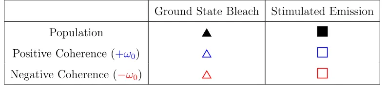
The population and coherence pathways for ground state bleach and stimulated emission
[image:16.612.109.506.487.575.2]processes are labelled using colour-coded symbols, as defined in table S1.
Table S1: Symbol Key for Liouville pathways.
Ground State Bleach Stimulated Emission
Population
Positive Coherence (+ω0)
Negative Coherence (−ω0)
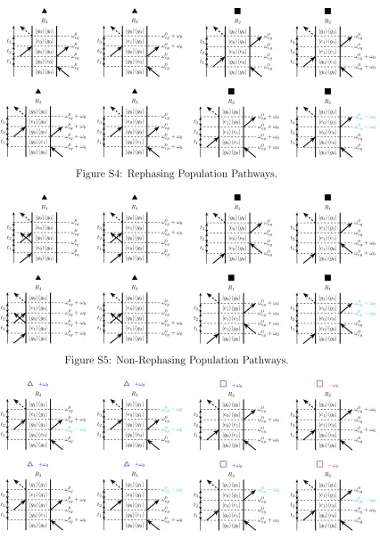
All 32 Liouville pathways are presented in figures S4 - S7 as double-sided Feynman
diagrams (see SI of reference 1). These diagrams are drawn in the usual manner, with the
t1 t2 t3 ω0 eg ω0 eg ω0 eg ω0 eg
|g0ihg0|
|g0ihe0|
|g0ihg0|
|e0ihg0|
|g0ihg0| R3 t1 t2 t3 ω0 eg ω0 eg ω0
eg+ω0 ω0
eg+ω0
|g0ihg0|
|g0ihe0|
|g0ihg0|
|e1ihg0|
|g0ihg0| R3 t1 t2 t3 ω0 eg ω0 eg ω0 eg ω0 eg
|g0ihg0|
|g0ihe0|
|e0ihe0|
|e0ihg0|
|g0ihg0| R2
t1 t2 t3
ω0
eg+ω0 ω0
eg+ω0 ω0
eg ω0
eg
|g0ihg0|
|g0ihe1|
|e1ihe1|
|e1ihg1|
|g1ihg1| R2
t1 t2 t3
ω0
eg+ω0 ω0
eg+ω0 ω0
eg+ω0 ω0
eg+ω0
|g0ihg0|
|g0ihe1|
|g0ihg0|
|e1ihg0|
|g0ihg0| R3
t1 t2 t3
ω0
eg+ω0 ω0
eg+ω0 ω0
eg ω0
eg
|g0ihg0|
|g0ihe1|
|g0ihg0|
|e0ihg0|
|g0ihg0| R3
t1 t2 t3
ω0
eg+ω0 ω0
eg+ω0 ω0
eg+ω0 ω0
eg+ω0
|g0ihg0|
|g0ihe1|
|e1ihe1|
|e1ihg0|
|g0ihg0| R2 t1 t2 t3 ω0 eg ω0 eg ω0
eg−ω0
ω0
eg−ω0
|g0ihg0|
|g0ihe0|
|e0ihe0|
|e0ihg1|
[image:17.612.108.534.67.672.2]|g1ihg1| R2
Figure S4: Rephasing Population Pathways.
t1 t2 t3 ω0 eg ω0 eg ω0 eg ω0 eg
|g0ihg0|
|e0ihg0|
|g0ihg0|
|e0ihg0|
|g0ihg0| R4 t1 t2 t3 ω0 eg ω0 eg ω0
eg+ω0 ω0
eg+ω0
|g0ihg0|
|e0ihg0|
|g0ihg0|
|e1ihg0|
|g0ihg0| R4 t1 t2 t3 ω0 eg ω0 eg ω0 eg ω0 eg
|g0ihg0|
|e0ihg0|
|e0ihe0|
|e0ihg0|
|g0ihg0| R1
t1 t2 t3
ω0
eg+ω0 ω0
eg+ω0 ω0
eg ω0
eg
|g0ihg0|
|e1ihg0|
|e1ihe1|
|e1ihg1|
|g1ihg1| R1
t1 t2 t3
ω0
eg+ω0 ω0
eg+ω0 ω0
eg+ω0 ω0
eg+ω0
|g0ihg0|
|e1ihg0|
|g0ihg0|
|e1ihg0|
|g0ihg0| R4
t1 t2 t3
ω0
eg+ω0 ω0
eg+ω0 ω0
eg ω0
eg
|g0ihg0|
|e1ihg0|
|g0ihg0|
|e0ihg0|
|g0ihg0| R4
t1 t2 t3
ω0
eg+ω0 ω0
eg+ω0 ω0
eg+ω0 ω0
eg+ω0
|g0ihg0|
|e1ihg0|
|e1ihe1|
|e1ihg0|
|g0ihg0| R1 t1 t2 t3 ω0 eg ω0 eg ω0
eg−ω0
ω0
eg−ω0
|g0ihg0|
|e0ihg0|
|e0ihe0|
|e0ihg1|
|g1ihg1| R1
Figure S5: Non-Rephasing Population Pathways.
t1 t2 t3 ω0 eg ω0
eg−ω0
ω0
eg+ω0 ω0
eg
|g0ihg0|
|g0ihe0|
|g0ihg1|
|e1ihg1|
|g1ihg1| R3 +ω0 t1 t2 t3 ω0 eg ω0
eg−ω0
ω0
eg
ω0
eg−ω0
|g0ihg0|
|g0ihe0|
|g0ihg1|
|e0ihg1|
|g1ihg1| R3 +ω0 t1 t2 t3 ω0
eg+ω0 ω0
eg ω0
eg+ω0 ω0
eg
|g0ihg0|
|g0ihe1|
|e0ihe1|
|e0ihg0|
|g0ihg0| R2 +ω0 t1 t2 t3 ω0 eg ω0
eg+ω0 ω0
eg ω0
eg+ω0
|g0ihg0|
|g0ihe0|
|e1ihe0|
|e1ihg0|
|g0ihg0| R2
−ω0
t1 t2 t3
ω0
eg+ω0 ω0
eg ω0
eg+ω0 ω0
eg
|g0ihg0|
|g0ihe1|
|g0ihg1|
|e1ihg1|
|g1ihg1| R3 +ω0 t1 t2 t3 ω0
eg+ω0 ω0
eg ω0
eg
ω0
eg−ω0
|g0ihg0|
|g0ihe1|
|g0ihg1|
|e0ihg1|
|g1ihg1| R3 +ω0 t1 t2 t3 ω0
eg+ω0 ω0
eg ω0
eg
ω0
eg−ω0
|g0ihg0|
|g0ihe1|
|e0ihe1|
|e0ihg1|
|g1ihg1| R2 +ω0 t1 t2 t3 ω0 eg ω0
eg+ω0
ω0
eg−ω0
ω0
eg
|g0ihg0|
|g0ihe0|
|e1ihe0|
|e1ihg1|
|g1ihg1| R2
−ω0
t1 t2 t3 ω0 eg ω0
eg−ω0
ω0
eg ω0
eg+ω0
|g0ihg0|
|e0ihg0|
|g1ihg0|
|e1ihg0|
|g0ihg0| R4
−ω0
t1 t2 t3 ω0 eg ω0
eg−ω0
ω0
eg−ω0
ω0
eg
|g0ihg0|
|e0ihg0|
|g1ihg0|
|e0ihg0|
|g0ihg0| R4
−ω0
t1 t2 t3
ω0
eg+ω0 ω0
eg ω0
eg ω0
eg+ω0
|g0ihg0|
|e1ihg0|
|e1ihe0|
|e1ihg0|
|g0ihg0| R1
−ω0
t1 t2 t3 ω0 eg ω0
eg+ω0 ω0
eg+ω0 ω0
eg
|g0ihg0|
|e0ihg0|
|e0ihe1|
|e0ihg0|
|g0ihg0| R1 +ω0 t1 t2 t3 ω0
eg+ω0 ω0
eg ω0
eg ω0
eg+ω0
|g0ihg0|
|e1ihg0|
|g1ihg0|
|e1ihg0|
|g0ihg0| R4
−ω0
t1 t2 t3
ω0
eg+ω0 ω0
eg
ω0
eg−ω0
ω0
eg
|g0ihg0|
|e1ihg0|
|g1ihg0|
|e0ihg0|
|g0ihg0| R4
−ω0
t1 t2 t3
ω0
eg+ω0 ω0
eg
ω0
eg−ω0
ω0
eg
|g0ihg0|
|e1ihg0|
|e1ihe0|
|e1ihg1|
|g1ihg1| R1
−ω0
t1 t2 t3 ω0 eg ω0
eg+ω0 ω0
eg
ω0
eg−ω0
|g0ihg0|
|e0ihg0|
|e0ihe1|
|e0ihg1|
|g1ihg1| R1
[image:18.612.109.530.73.248.2]+ω0
Figure S7: Non-Rephasing Coherence Pathways.
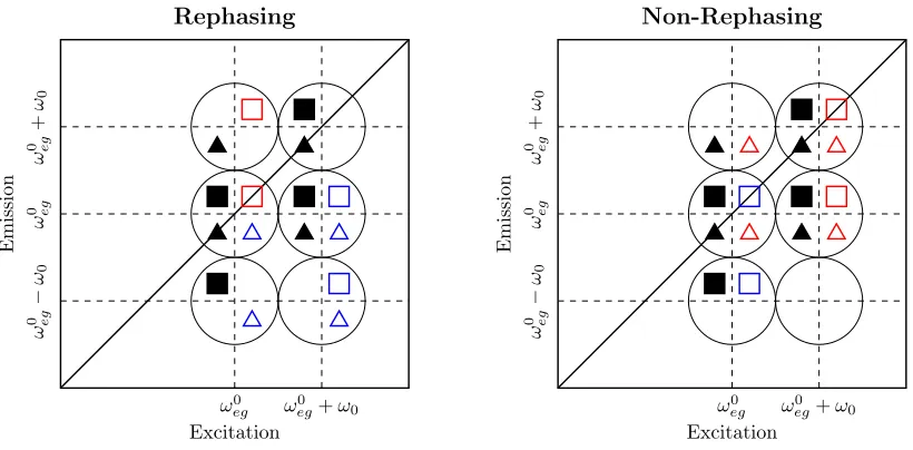
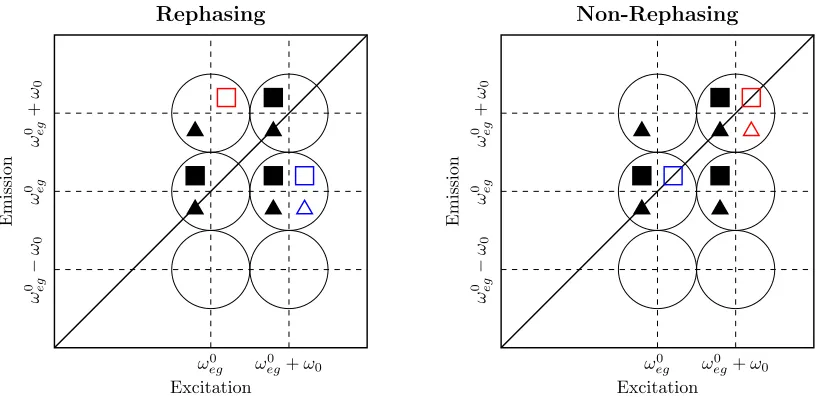
For the centred laser spectrum simulation, all 32 pathways contribute, with the peak
locations predicted as shown in figure S8 for the rephasing and non-rephasing spectra. Here
the population pathways have been included, identifying peak locations to which they would
contribute, were they not removed from the amplitude spectra by the exponential fitting
procedure, as described above.
ω0
eg ω
0
eg+ω0
ω 0 eg ω 0 eg + ω0 ω 0 eg − ω0 Rephasing E m is si on Excitation ω0 eg ω 0
eg+ω0
ω 0 eg ω 0 eg + ω0 ω 0 eg − ω0 Non-Rephasing E m is si on Excitation
[image:18.612.104.514.414.616.2]On blue-shifting the laser spectrum, all pathways involving the ω0
eg−ω0 transition
fre-quency (highlighted cyan in figures S4 - S7) are eliminated from the spectra. This results
in the loss of the lower emission frequency peaks from the amplitude spectra, as shown in
figure S9.
ω0
eg ω
0
eg+ω0
ω
0 eg
ω
0 eg
+
ω0
ω
0 eg
−
ω0
Rephasing
E
m
is
si
on
Excitation
ω0
eg ω
0
eg+ω0
ω
0 eg
ω
0 eg
+
ω0
ω
0 eg
−
ω0
Non-Rephasing
E
m
is
si
on
[image:19.612.104.514.172.374.2]Excitation
Figure S9: Peak location key diagram for the blue-shifted laser spectrum simulation, includ-ing population pathways, for Rephasinclud-ing (left) and Non-Rephasinclud-ing (right) amplitude spectra. The Liouville pathways are identified as per table S1, producing peaks in the spectra iden-tified by the encompassing black circles.
Additional 2D Spectra Examples
Summaries of calculated rephasing and non-rephasing 2D spectra (real, normalised) for both
~
ωt
/
10
3cm
−
1
T= 0 fs T= 50 fs
Rephasing (Real)
T= 100 fs
~
ωt
/
10
3cm
−
1
~ωτ /103cm−1
T= 200 fs
~ωτ /103cm−1
T= 400 fs
~ωτ /103cm−1
[image:20.612.95.514.74.312.2]T= 800 fs
Figure S10: Rephasing (real) spectra for the centred laser spectrum simulation.
~
ωt
/
10
3cm
−
1
T= 0 fs T= 50 fs
Non-Rephasing (Real)
T= 100 fs
~
ωt
/
10
3cm
−
1
~ωτ /103cm−1
T= 200 fs
~ωτ /103cm−1
T= 400 fs
~ωτ /103cm−1
T= 800 fs
[image:20.612.96.514.371.609.2]~
ωt
/
10
3cm
−
1
T= 0 fs T= 50 fs
Rephasing (Real)
T= 100 fs
~
ωt
/
10
3cm
−
1
~ωτ /103cm−1
T= 200 fs
~ωτ /103cm−1
T= 400 fs
~ωτ /103cm−1
[image:21.612.94.514.74.311.2]T= 800 fs
Figure S12: Rephasing (real) spectra for the blue-shifted laser spectrum simulation.
~
ωt
/
10
3cm
−
1
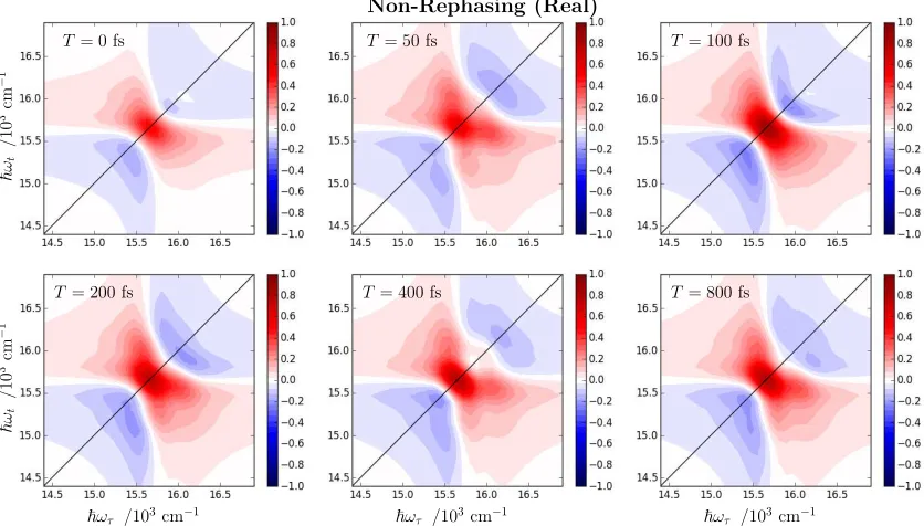
T= 0 fs T= 50 fs
Non-Rephasing (Real)
T= 100 fs
~
ωt
/
10
3cm
−
1
~ωτ /103cm−1
T= 200 fs
~ωτ /103cm−1
T= 400 fs
~ωτ /103cm−1
T= 800 fs
Figure S13: Non-Rephasing (real) spectra for the blue-shifted laser spectrum simulation.
[image:21.612.94.515.359.592.2]Computational Details
The evolution of the auxiliary density operators is solved using the fourth order Runge-Kutta
method and FORTRAN 90, with a time step of 0.05 fs. Construction of the system and all
other manipulations were performed using Python, making use of the standard NumPy and
matplotlib packages, as well as the quantum object class of the QuTiP (Quantum Toolbox
in Python) package.20,21
References
(1) Camargo, F. V. A.; Grimmelsmann, L.; Anderson, H. L.; Meech, S. R.; Heisler, I. A.
Resolving Vibrational from Electronic Coherences in Two-Dimensional Electronic
Spec-troscopy: The Role of the Laser Spectrum. Phys. Rev. Lett. 2017,118, 033001.
(2) Camargo, F. V. A.; Anderson, H. L.; Meech, S. R.; Heisler, I. A. Full Characterization
of Vibrational Coherence in a Porphyrin Chromophore by Two-Dimensional Electronic
Spectroscopy. J. Phys. Chem. A2015,119, 95–101.
(3) Drobizhev, M.; Stepanenko, Y.; Dzenis, Y.; Karotki, A.; Rebane, A.; Taylor, P. N.;
An-derson, H. L. Extremely Strong Near-IR Two-Photon Absorption in Conjugated
Por-phyrin Dimers: Quantitative Description with Three-Essential-States Model. J. Phys.
Chem. B 2005, 109, 7223–7236.
(4) Camargo, F. V. A. Unravelling Vibrational and Electronic Coherences via
Two-Dimensional Electronic Spectroscopy of Zinc-Porphyrins. Ph.D. thesis, University of
East Anglia, 2017.
(5) Kim, S. Y.; Joo, T. Coherent Nuclear Wave Packets in Q States by Ultrafast Internal
Conversions in Free Base Tetraphenylporphyrin. J. Phys. Chem. Lett. 2015, 6, 2993–
(6) Mukamel, S. Principles of Nonlinear Optical Spectroscopy; Oxford University Press:
New York, 1995.
(7) Dijkstra, A. G.; Tanimura, Y. Linear and Third- and Fifth-Order Nonlinear
Spectro-scopies of a Charge Transfer System Coupled to an Underdamped Vibration.J. Chem.
Phys. 2015, 142, 212423.
(8) Tanimura, Y. Stochastic Liouville, Langevin, Fokker-Planck, and Master Equation
Ap-proaches to Quantum Dissipative Systems. J. Phys. Soc. Jpn. 2006,75, 082001.
(9) Chen, L.; Zheng, R.; Shi, Q.; Yan, Y. Optical Line Shapes of Molecular Aggregates:
Hierarchical Equations of Motion Method.J. Chem. Phys. 2009, 131, 094502.
(10) Dijkstra, A. G.; Tanimura, Y. System Bath Correlations and the Nonlinear Response
of Qubits. J. Phys. Soc. Jpn. 2012, 81, 063301.
(11) Dijkstra, A. G.; Prokhorenko, V. I. Simulation of Photo-Excited Adenine in Water with
a Hierarchy of Equations of Motion Approach. J. Chem. Phys. 2017, 147, 064102.
(12) Tanimura, Y. Reduced Hierarchy Equations of Motion Approach with Drude plus
Brow-nian Spectral Distribution: Probing Electron Transfer Processes by means of
Two-Dimensional Correlation Spectroscopy. J. Chem. Phys. 2012, 137, 22A550.
(13) Brixner, T.; Manˇcal, T.; Stiopkin, I. V.; Fleming, G. R. Phase-Stabilized
Two-Dimensional Electronic Spectroscopy. J. Chem. Phys. 2004, 121, 4221–4236.
(14) Sharp, L. Z.; Egorova, D.; Domcke, W. Efficient and Accurate Simulations of
Two-Dimensional Electronic Photon-Echo Signals: Illustration for a Simple Model of the
Fenna-Matthews-Olson Complex. J. Chem. Phys. 2010, 132, 014501.
(15) Leng, X.; Yue, S.; Weng, Y.-X.; Song, K.; Shi, Q. Effects of Finite Laser Pulse Width
(16) Gelin, M. F.; Egorova, D.; Domcke, W. Efficient Method for the Calculation of
Time-and Frequency-Resolved Four-Wave Mixing Signals Time-and its Application to Photon-Echo
Spectroscopy. J. Chem. Phys. 2005, 123, 164112.
(17) Gelin, M. F.; Egorova, D.; Domcke, W. Efficient Calculation of Time- and
Frequency-Resolved Four-Wave-Mixing Signals. Acc. Chem. Res. 2009, 42, 1290–1298.
(18) Cheng, Y.-C.; Lee, H.; Fleming, G. R. Efficient Simulation of Three-Pulse Photon-Echo
Signals with Application to the Determination of Electronic Coupling in a Bacterial
Photosynthetic Reaction Center .J. Phys. Chem. A 2007, 111, 9499–9508.
(19) Cheng, Y.-C.; Engel, G. S.; Fleming, G. R. Elucidation of Population and Coherence
Dynamics using Cross-Peaks in Two-Dimensional Electronic Spectroscopy.Chem. Phys.
2007, 341, 285–295.
(20) Johansson, J.; Nation, P.; Nori, F. QuTiP: An Open-Source Python Framework for the
Dynamics of Open Quantum Systems.Comput. Phys. Commun.2012,183, 1760–1772.
(21) Johansson, J.; Nation, P.; Nori, F. QuTiP 2: A Python Framework for the Dynamics