systems
.
White Rose Research Online URL for this paper:
http://eprints.whiterose.ac.uk/122382/
Version: Accepted Version
Article:
Genes, C., Esnaola, I. orcid.org/0000-0001-5597-1718, Perlaza, S.M. et al. (2 more
authors) (2018) Robust recovery of missing data in electricity distribution systems. IEEE
Transactions on Smart Grid. ISSN 1949-3053
https://doi.org/10.1109/TSG.2018.2848935
© 2018 IEEE. Personal use of this material is permitted. Permission from IEEE must be
obtained for all other users, including reprinting/ republishing this material for advertising or
promotional purposes, creating new collective works for resale or redistribution to servers
or lists, or reuse of any copyrighted components of this work in other works. Reproduced
in accordance with the publisher's self-archiving policy.
[email protected] https://eprints.whiterose.ac.uk/
Reuse
Items deposited in White Rose Research Online are protected by copyright, with all rights reserved unless indicated otherwise. They may be downloaded and/or printed for private study, or other acts as permitted by national copyright laws. The publisher or other rights holders may allow further reproduction and re-use of the full text version. This is indicated by the licence information on the White Rose Research Online record for the item.
Takedown
If you consider content in White Rose Research Online to be in breach of UK law, please notify us by
Robust Recovery of Missing Data in Electricity
Distribution Systems
Cristian Genes, I˜naki Esnaola, Samir M. Perlaza, Luis F. Ochoa, and Daniel Coca.
Abstract—The advanced operation of future electricity distri-bution systems is likely to require significant observability of the different parameters of interest (e.g., demand, voltages, currents, etc.). Ensuring completeness of data is, therefore, paramount. In this context, an algorithm for recovering missing state variable observations in electricity distribution systems is presented. The proposed method exploits the low rank structure of the state variables via a matrix completion approach incorporating prior knowledge in the form of second order statistics. Essentially, the recovery method combines nuclear norm minimization with Bayesian estimation. The performance of the new algorithm is compared to the information-theoretic limits and tested through simulations using actual data of an urban low voltage distribution system. The impact of the prior knowledge is analyzed when a mismatched covariance is used and under a Markovian sampling that introduces structure in the observation pattern. Numerical results demonstrate that the proposed algorithm is robust and outperforms existing state of the art algorithms.
Index Terms—recovery of missing data, distribution systems, matrix completion, Bayesian estimation
I. INTRODUCTION
T
HE wide-spread adoption of residential scale low carbon technologies, such as photovoltaic systems and electric vehicles, undoubtedly brings technical challenges to the elec-tricity distribution systems. This is because these systems have been designed for passive loads, see [1] and [2]. From the standpoint of the smart grid vision, electricity distribution systems including low voltage (LV) circuits, are likely to adopt more active roles so as to cost-effectively manage controllable network elements and participants [3]. As a result, monitoring and control procedures are expected to face increasingly de-manding performance requirements posed by the dynamic and unknown scenarios that the smart grid gives rise to. Advanced control strategies require timely and accurate data describing the state of the grid. In this setting, the sensing infrastructure is expected to provide complete and reliable state information of the distribution system. However, in practical scenarios,Cristian Genes and Daniel Coca are with the Department of Automatic Control and Systems Engineering, University of Sheffield, Sheffield S1 3JD, UK.
I˜naki Esnaola is with the Department of Automatic Control and Systems Engineering, University of Sheffield, Sheffield S1 3JD, UK, and also with the Department of Electrical Engineering, Princeton University, Princeton NJ 08540, USA.
Samir M. Perlaza is with the Institut National de Recherche en Informatique et Automatique (INRIA), Lyon, France, and also with the Department of Electrical Engineering, Princeton University, Princeton NJ 08540, USA.
Luis F. Ochoa is with the Department of Electrical and Electronic En-gineering, The University of Melbourne, Melbourne 3010, Australia, and also with the School of Electrical and Electronic Engineering, The Univer-sity of Manchester, Manchester M13 9PL, UK. ([email protected], [email protected], [email protected], luis [email protected], and [email protected]).
the operator faces challenges like data injection attacks [4], [5] or missing data [6], [7]. Sensor failures, unreliable com-munication or data storage issues are some of the causes for incomplete sets of observations. As a consequence, the state of the grid is not perfectly known and control mechanisms are difficult to implement. For instance, accurate measurements are necessary to implement a centralized control scheme for voltage regulation in distribution systems [8]. In view of this, it is vital to develop estimation procedures for the missing data using the available observations.
Missing data recovery can be cast as a minimum mean square error (MMSE) estimation problem when a probabilistic description of the underlying process governing the state variables is available. However, the MMSE estimation relies on accurate second order statistics which is an unrealistic assumption in practical scenarios [7], [9]. The increased num-ber of nonlinear loads and the turbulent nature of distributed generation options in the locally controlled grid affects the precision of the postulated statistics for the state variables. For that reason, the efficiency of MMSE estimation is limited in the smart grid context [7].
Matrix completion (MC) was recently proposed to recover missing data from partial observations [10]. The main advan-tage is that the recovery via MC requires mild assumptions about the setting, e.g. access to second order statistics is not required. Instead, matrix completion-based recovery exploits the fact that correlated state variable vectors give rise to approximately low rank data matrices. That being the case, the recovery of the missing entries of low rank matrices is feasible in a convex optimization context provided that a sufficient fraction of the entries is observed [10], [11], and [12]. The key theoretical results therein are based on the assumption that the locations of sampled entries are uniformly distributed. In practice, however, this assumption is not always satisfied. For instance, in electricity distribution systems, missing data entries tend to display significant structure across both space and time [7]. The applicability of MC recovery for non-uniform sampling is studied in [6] and [13]. Not surprisingly, low rank minimization tools are also used to address the problem of electricity price forecasting [14] and to develop a framework for efficient processing of synchrophasor data [6]. However, the nature of synchrophasor data is different from the LV distribution data used in this work. In particular, data describing the state variables of a LV distribution system exhibits lower temporal resolution and significant correlation that permits modeling the state variables as a stochastic process.
algorithm is the low computational cost which allows the use matrices with up to one billion entries [15]. On the other side, the main shortcoming of SVT is that it requires parameter tuning for the thresholding step and there are no guidelines for choosing the optimal value. In [16] the problem of opti-mal soft-thresholding is addressed using Stein's unbiased risk estimate (SURE) [17] where a closed-form expression for the performance of the soft-thresholding step is provided in a denoising framework.
This paper proposes an information-theoretic framework for assessing the performance of missing data recovery tech-niques in electricity distribution grids. The advantage of this viewpoint is twofold. First, the fundamental limits of missing data recovery in electricity distribution systems are characterized. As a result, the optimal performance attainable by a given sensing infrastructure can be specified. Secondly, existing missing data recovery algorithms can be benchmarked against the fundamental limits. On the other hand, operational regimes in which the performance is largely suboptimal can be identified. In view of this, a novel algorithm for recovering missing data in electricity distribution systems is presented. The proposed recovery method is based on SVT [15] and ad-dresses two distinct challenges posed by electricity distribution systems:
• Practical missing data patterns do not follow independent and identically distributed observation patterns,
• The sensing infrastructure introduces noise.
The proposed algorithm addresses these challenges by provid-ing an adaptive thresholdprovid-ing based on second order statistics. To that end, the addition of a MMSE estimation step makes possible the use of SURE [17] in a missing data recovery setting. The performance of the new algorithm is tested against SVT recovery [15] and MMSE estimation under realistic assumptions, i.e., the postulated statistics are not accurate and the sampling pattern is not uniform. Numerical results show a significant gain in performance for both cases when compared to SVT recovery. Remarkably, the proposed algorithm is robust to mismatched second order statistics which suggests that accurate statistics are not required to recover missing LV data in electricity distribution systems.
II. SYSTEM MODEL
Consider a LV distribution system with L feeders. Each feeder includes a sensing unit that measures the electrical magnitudes of operational interest at predetermined time in-stants. These measurements that include phase active power, phase reactive power and phase voltage support the operator in controlling, monitoring, and managing the network. In practice, the acquisition process provides the operator with a noisy and incomplete set of state variables. For that reason, the operator needs to recover the missing LV data using the available observations.
A. Source Model for State Variables
For a given electrical magnitude s, let m(i,js) be the
cor-responding value at feeder i ∈ {1,2, ..., L} at time j ∈
0 50 100 150 200 250 300 350
[image:3.612.318.545.64.238.2]10-4 10-2 100 102 104
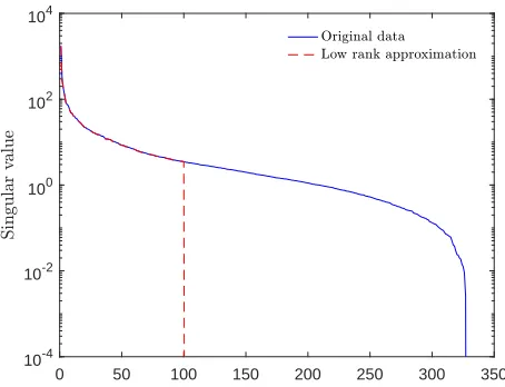
Figure 1. Singular values of the matrixMcontaining the voltage measure-ments, whenN=L= 500, compared to a low-rank approximation of the same matrix when the rank is one hundred.
{1,2, ..., N}. The matrix of state variables for magnitudes, de-noted byM(s)∈RN×L, contains the aggregated state variable
vectors from all feeders, i.e. M(s) ∆= [m(s) 1 ,m
(s) 2 , ...,m
(s) L ]
where,m(s)
i = [m (s) i,1, m
(s) i,2, ..., m
(s) i,N]
T ∈RN. Without loss of
generality the analysis is carried out for a particular electrical magnitude, and therefore, the indexsis dropped. The resulting data matrix M contains the state variable of interest at time
instants1,2, ..., N for allLfeeders.
Actual LV data is used to model the statistical structure of the data generated in a low voltage electricity distri-bution system. The actual LV data set under consideration contains values from 200 residential secondary substations across the North West of England collected from June 2013 to January 2014. The data collection is part of the “Low Voltage Network Solutions” project run by Electricity North West Limited [18]. Each substation creates a daily file containing values of voltage, current and power levels for all three phases. An analysis of the distribution and sample covariance matrix of the voltage measurements in the LV data set under consideration is presented in [7]. Therein, it is shown that state variables can be modelled as a multivariate Gaussian random process, more specifically for alli ∈ {1,2, ..., L}, it holds that
mi∼N(µ,Σ), (1)
and mi is a sequence of independent and identically
dis-tributed random variables. Consequently,Mis a realization of
the random process describing the value of the state variable of interest across the grid. The significant correlation among the state variables observed in the LV data set induces a large condition number [19] in the singular value decomposition, i.e. there are a few singular values that concentrate most of the norm of the matrix, and therefore, the matrix can be modelled as approximately low rank, see [10], [11], and [12]. That being the case, the truncated low-rank approximation of the matrix obtained by setting the rank(M)−Ksmallest singular values
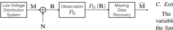
Low Voltage Distribution
System
Missing Data Recovery Observation
PΩ
N
[image:4.612.50.341.54.106.2]M R PΩ(R) cM
Figure 2. Block diagram describing the system model.
some values of K. For instance, Fig. 1 depicts the singular values, in decreasing order, of the matrix M. It also shows
the singular values of a low rank approximation of the same matrix. Interestingly, the first five singular values in decreasing order concentrate 98.78% of the matrix nuclear norm while the first thirty singular values concentrate99.4%of the matrix nuclear norm. This justifies posing the recovery problem as a rank minimization problem. It is important to note that the recovery strategies analyzed do not impose constraints on the minimum number of observations per column. In contrast, the information cascading matrix completion (ICMC) based recovery in [6] operates under the assumption that there is a minimum number of observations per column which is lower bounded by the rank [20]. Moreover, the ICMC recovery requires knowledge of the rank of the matrix to be estimated [20] which is not a realistic assumption in a practical scenario. Fig. 2 describes the distribution system monitoring model. In this setting, the electrical magnitudes describing the state of the system are modelled as a random process that outputs a realization M ∈ RN×L every N time instants. The state
of the grid is fully described by the entries of the matrix
M. However, the operator observes a subset of the complete
set of state variables, i.e. measurements are lost during the acquisition process. The aim of the estimation process is to recover the missing entries.
B. Acquisition
The sensing infrastructure introduces additive white Gaus-sian noise (AWGN) as a result of the thermal noise present at each sensor. The resulting measurements are given by
R=M+N, (2)
where
(N)i,j∼ N(0, σ2), (3)
for i ∈ {1,2, ..., N} and j ∈ {1,2, ..., L}. Moreover, it is also assumed that only a fraction of the complete set of measurements (entries in R) are communicated to the
operator. Denote by Ω the subset of observed entries, i.e., Ω⊆ {1,2, ...N} × {1,2., ..., L}. By definition it follows that Ωis given by
Ω=∆{(i, j) : (R)i,j is observed}. (4)
Formally, the acquisition process is modelled by the function f :RN×L→R|⌦|withf(M) =P⌦(R)where
P⌦(R) = (R)⌦, (5)
and |Ω|denotes the cardinality of Ω. The observations given by (5) describe all the data that is available to the operator for estimation purposes and therefore, the recovery of the missing data is performed from the observationsP⌦(R).
C. Estimation
The estimation process of the complete matrix of state variables based on the available observations is modelled by the function g:R|⌦|→RN×L. The estimateMc=g(f(M))
is obtained by solving an optimization problem based on an optimality criterion. In this paper, the optimality criterion is the mean square error (MSE) given by
MSE(M;g) = E
kM−g(f(M))k2 F
N L , (6)
wherek·kFdenotes the Frobenius norm. The normalized mean
square error (NMSE) is defined as
NMSE(M;g) =MSE(M;g) N L
kMk2 F
. (7)
For this optimality criterion, the optimal estimate of the missing data is given by the MMSE estimate
c
MMMSE=E[M|f(M),Σ], (8)
where Σ ∈ RN×N is the covariance matrix defined in (1).
Note that, in general, obtaining the optimal estimate cMMMSE
requires knowledge of the probability distribution describing the state variables. If the state variables follow a Gaussian distribution it boils down to the knowledge of the second order moments, i.e. the covariance matrixΣwhich needs to be
known prior to the estimation process. In practice, the operator relies on postulated statistics that typically do not match the actual statistics. Consequently, the accuracy of the estimate is a function of the difference between the real and the postulated statistics.
III. INFORMATION-THEORETICLIMIT
In order to assess the performance of the missing data recovery techniques in absolute terms, this section introduces the optimal performance theoretically attainable (OPTA) by an estimator g when the state variables follow a multivariate Gaussian distribution. For a given number of observations, the minimum distortion achievable by any estimation method is determined by the rate-distortion function [21]. In the electric-ity distribution setting described above, the observations are corrupted by additive white Gaussian noise which determines the finite rate at which information about the state variables is obtained. Consequently, the optimal performance is bounded by the capacity of the AWGN channel, denoted byC, i.e.,
R(D)< C, (9)
whereR is the rate at which the source needs to be observed to achieve a distortion D. In view of this, the OPTA for a multivariate Gaussian source is given by
R(D)≤ |Ω|
2N Llog10(1 +snr), (10) where the signal to noise ratio, denoted bysnr, is defined as
snr=∆ 1 NTr(Σ)
where σ2 is defined in (3). The rate-distortion function of a
multivariate Gaussian process is computed using the following parametric equations [22]
(
R(θ) = N1 PNi=0−1max(0, 1 2log
λi
θ)
D(θ) = 1 N
PN−1
i=0 min(θ, λi),
(12)
where R is the source rate in nats/symbol, D is the mean square error distortion per entry, λi is the ith largest
eigen-value of Σ, and θ is a parameter. The NMSE theoretically
attainable, NMSE(M;OPTA), follows from combining (7) and
(12) and is determined by
NMSE(M;OPTA) =D N L
kMk2 F
. (13)
IV. RECOVERY OF MISSING DATA
In this section, the information-theoretic limit for missing data recovery presented in Section III, is compared with MMSE estimation and the singular value thresholding (SVT) recovery.
A. Minimum Mean Squared Error Estimation
Linear MMSE (LMMSE) estimation achieves the optimal performance in the recovery of missing data for a given set of observations Ωwhen the data is generated by a multivariate Gaussian source and the optimality criteria is the MSE. However, this estimation procedure relies on access to second order statistics of the state variables. In particular, the available entries from the columni of the matrixRare given by
P⌦(ri) =Ai(mi+ni), (14)
where Ai is defined such that Aimi = P⌦(mi) and i ∈
{1,2, ..., L}. Consequently, the LMMSE estimate for each state variable vector is given by
b
mi=µ+Γi(P⌦(ri)−Aiµ), (15)
whereµis defined in (1) and
Γi =ΣATi(AiΣATi +σ2I)−1, (16)
i ∈ {1,2, ..., L}. The normalized error achieved by the LMMSE estimator is given by
NMSE(M;LMMSE) =kM−McLMMSEk 2 F
kMk2 F
, (17)
whereMcLMMSE= [mb1,mb2, ...,mbL], withmbidefined in (15).
B. Singular Value Thresholding
Low rank matrices are recovered from a subset of the entries via rank minimization techniques under mild coherence conditions on the set of observations [10]. Specifically, the missing entries are recovered by solving the following rank minimization problem:
minimize
X rank(
X)
subject to P⌦(X) =P⌦(M).
(18)
Unfortunately, this rank minimization problem is NP-hard. Favorably, in [10] it is shown that when the entries on Ω are sampled uniformly at random, the solution of the rank minimization problem in (18) is obtained with high probability by solving the nuclear norm minimization problem in (20).
SVT is a matrix completion algorithm [15] which produces a sequence of matrices Xk that converges to the unique
solution of the following optimization problem:
minimize X τk
Xk∗+1
2kXk
2 F
subject to P⌦(X) =P⌦(M),
(19)
wherekXk∗ is the nuclear norm of the matrix X. Note that
when τ→ ∞, the optimization problem in (19) converges to the nuclear norm minimization problem proposed in [10]
minimize
X k
Xk∗
subject to P⌦(X) =P⌦(M).
(20)
For large values of τ, SVT provides the solution to the nuclear norm minimization problem. Compared to alternatives like SeDuMi [23] or SDPT3 [24], SVT features a lower computational cost per iteration. This is achieved by exploiting the sparsity ofYk and the low-rank property ofXk to reduce
storage requirements. The low computational cost results in the possibility of using larger matrices. Simulation results in [15] show that SVT recovers matrices with nearly a billion entries. In comparison, SeDuMi and SDPT3 produce accurate solutions for squared matrices with dimension close to fifty. In [25] the structure of the problem is exploited to reduce the memory requirements and increase the matrix size up to 350. Because of the dimension of the data sets produced by low voltage distribution systems, the remaining of the paper focuses on the SVT as a benchmark MC-based recovery. The main idea in SVT consists in the following iteration steps:
(
Xk=D
τ(Yk−1),
Yk =Yk−1+δs P⌦(M)−P⌦(Xk),
(21)
whereY0=0,δs is the step size that obeys0< δs<2, and
the soft-thresholding operator,Dτ, applies a soft-thresholding
rule to the singular values of Yk−1, shrinking these towards
zero. Note that the index k is not a power but an iteration index. For a matrixY∈RN×L of rankrwith singular value decomposition given by
Y=USVT, S=diag({σi(Y)}1≤i≤r), (22)
whereUandVare unitary matrices of sizeN×randL×r,
respectively, and σi(Y)are the singular values of the matrix
Y, the soft-thresholding operator is defined as
Dτ(Y) ∆
=UDτ(S)VT, withDτ(S) =diag({(σi(Y)−τ)+}),
(23) where t+ = max(0, t). Interestingly, the choice of τ is
important to guarantee a successful recovery, since large values guarantee a low-rank matrix estimate but for values larger than max
i (σi(
Y)) all the singular values vanish. In [15],
0 0.2 0.4 0.6 0.8 1 10-8
[image:6.612.55.294.66.256.2]10-6 10-4 10-2
Figure 3. LV data recovery performance using SVT, LMMSE estimation, for different levels of mismatch, and the OPTA, when SNR= 20dB.
performance when the number of missing entries is large. The choice of τ governs the performance trade-off between the high and low sampling regimes. Large values ofτyield a good performance when a small number of observations is available. Conversely, smaller values of τ yield a good performance when a large number of observations is available. Unfortu-nately, finding the optimal threshold when the matrix is sparse is still an open problem. In general, the value of the threshold for soft-thresholding based recovery algorithms is obtained via numerical optimization in [7] and [12]. The same soft-thresholding operator,Dτ, is used in a different framework for
denoising [12], [26], and [27]. In this context, the performance of the denoiser, measured in MSE, is estimated using Stein's unbiased risk estimate (SURE) [17]. In [16] a closed-form expression for the unbiased risk estimate is presented for the operatorDτ.
C. Performance Evaluation with Actual LV Data
This subsection presents a comparison between LMMSE and SVT, and the theoretical limit, OPTA, using actual LV data. The test matrix, M, is a square matrix of size 500, i.e.
N =L = 500, and contains voltage measurements covering the state of the grid for a period of 2 hours. Each column represents a different state variable vector that describes the grid on a different day and for a different feeder. The entries inΩare sampled uniformly at random with probability
P[(i, j)∈Ω] = 1
N LE[|Ω|], (24) and the performance of the SVT-based recovery is defined in terms of the NMSE given by
NMSE(M;SVT) = kM−cMSVTk 2 F
kMk2F , (25)
wherecMSVTis the SVT estimate ofMbased onP⌦(R). Let
γ be the ratio of missing entries for the matrixM, that is:
γ∆= 1− 1
N L|Ω|. (26)
Since the performance of the LMMSE estimator depends on the covariance matrix Σ, a mismatched covariance matrix
model [28] and [29] is introduced to account for the difference between the postulated and actual statistics. Specifically, the postulated covariance matrix is given by
Σ∗=Σ+ 1
SMR
kΣk2F
k∆k2 F
∆, (27)
where Σ is the actual covariance matrix in (1), ∆=HHT
withH∈RN×N any matrix whose entries are distributed as
N(0,1). The strength of the mismatch is determined by the signal to mismatch ratio (SMR), which is defined such that for SMR= 1 the norm of the mismatch is equal to the norm of the real covariance matrix, i.e.,kΣk2
F =k 1 SMR
kΣk2
F
k∆k2
F ∆k2
F.
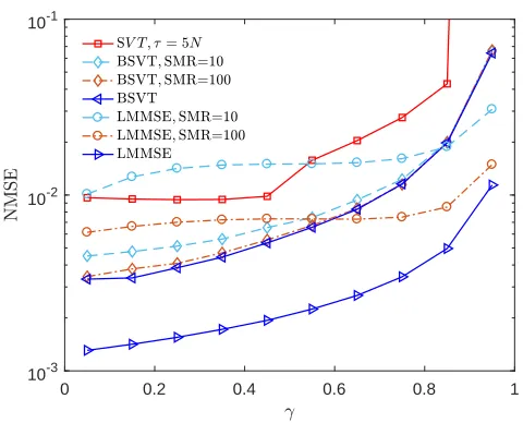
Fig. 3 shows the performance, measured in NMSE, for the SVT-based recovery compared to the performance of the LMMSE estimator when different levels of mismatch are introduced and to the theoretical limit given by the OPTA. Numerical results in this section are obtained for a signal to noise ratio value of SNR= 20dB, where SNR= 10∆ log10snr.
It can be seen that the performance of the SVT algorithm is closer to the theoretical limit when the number of missing entries is large. Interestingly, the LMMSE estimator gives bet-ter performance when SMR≥100. However, when SMR=10 and γ ≤ 0.55 the SVT algorithm outperforms the LMMSE estimator. Moreover, the SVT provides a better recovery for SMR=1 for almost all values ofγ. In view of this, the LMMSE estimation requires accurate second order statistics to perform competitively in this setting which is an unrealistic assumption in a practical scenario. Moreover, the performance of the SVT algorithm depends of the threshold τ [7] which is difficult to optimize for this case.
V. MAINRESULT
This section introduces a novel algorithm for missing data recovery that incorporates imperfect second order statistics. The new approach is based on the SVT algorithm but it exploits the information about the second order statistics to optimize the thresholdτ at each iteration k.
A. Soft-thresholding parameter
B. Exploiting second order statistics
In order to overcome the limitation imposed by the sparse structure of the matrix Yk
, the proposed algorithm estimates the missing entries prior to the soft-thresholding step. Thus, the available prior knowledge is exploited to produce an estimate of the entries not contained inΩ. In this case, at each iteration k of the proposed algorithm the matrixZk is computed as
Zk=Yk+Lk, (28)
where Yk is defined as in the SVT algorithm and Lk is the
LMMSE estimate given by
Lk =P⌦c(µ) +Σ⌦c⌦Σ−1
⌦⌦(P⌦(Yk)−P⌦(µ)), (29)
whereΩis the set of observed entries,Ωc
is the set of missing entries,Σ⌦c
⌦is the covariance matrix between the entries in
Ωc
and the entries in Ω and Σ⌦⌦ is the covariance matrix
of the entries in Ω. In a nutshell, the unknown entries are estimated using the LMMSE-based recovery at each iteration k. The result is a complete matrixZk
for which the tuning of the threshold is feasible.
C. Optimization of thresholding parameter
Following the brief discussion in Section IV-B, the closed-form expression for the risk estimator provided in [16] is incorporated into the proposed algorithm. The use of SURE is made possible by the addition of the LMMSE step, which provides a linear estimation for the entries inΩc. This ensures
that the matrix provided as input to the soft-thersholding step is complete and the optimization of τ is solvable as a denoising problem. In this context, the performance of the soft-thresholding operator can be estimated when the input matrix accepts the following model [16]
Z=M+W, (30)
where the entries ofW are
(W)i,jiid∼ N(0, σ2
Z), (31)
for i∈ {1,2, ..., N} andj ∈ {1,2, ..., L}. In this setting, the SURE [17] is given by
SURE(Dτ)(Z) =−N Lσ2Z+
min(N,L)
X
i=1
min(τ2, σ2 i(Z))
+ 2σZ2div(Dτ(Z)),
(32)
where σi(Z) is the i-th singular value of Z for i ∈
{1,2, . . . , N}. A closed-form expression for the divergence of this estimator is obtained in [16]. For the case in which
Z∈RN×L the divergence is given by
div(Dτ(Z)) =
min(N,L)
X
i=1
I(σi(Z)> τ) +|N−L|
(σi(Z)−τ)+
σi(Z)
+ 2
min(N,L)
X
i6=j,i,j=1
σi(Z)(σi(Z)−τ)+
σ2
i(Z)−σ2j(Z)
,
(33)
whenZhas no repeated singular values and is zero otherwise.
Therefore, combining (32) and (33) gives a closed-form ex-pression for the performance of the soft-thresholding operator for different values of τ and different noise levelsσ2
Z. The proposed algorithm approximatesσ2
Zwith the weighted sum of the noise in Ω and in Ωc
. Consequently, σ2
Zk is
calculated as
σ2Zk=
kYk−P
⌦(M)k2F+|Ωc|DLMMSE
N L , (34)
whereDLMMSE represents the average noise per entry in Ωc.
The optimal threshold for the matrixZk is denoted byτ∗k and
it is calculated using
τk
∗ =arg min
τ
SURE(Dτ)(Zk), (35)
whereσ2
Zk is given by (34).
Note that the cost function in (35) is quasiconvex and is solved using standard optimization tools [16] over a predefined interval [τmin, τmax]. Therefore, the iterations of the proposed
algorithm are
Xk=D
τ(Zk−1),
Yk =Yk−1+δb P⌦(M)−P⌦(Xk), Zk =Yk+Lk,
(36)
where theDτ is defined by (23) and the step sizeδb is similar
to the step sizeδsin the SVT algorithm. The initial conditions
are Z0 = 0, Y0 = 0 and τ = 0. The stopping criteria is
similar to the SVT algorithm, namely
kP⌦(Xk−M)kF
kP⌦(M)kF
≤ǫ. (37) A more detailed description of the proposed algorithm is presented in Algorithm 1.
Algorithm 1 Bayesian Singular Value Thresholding
Input: observations setΩ, and observed entriesP⌦(R), mean
µ, covariance matrix Σ, step size δb, tolerance ǫ, and
maximum iteration count kmax
Output: McBSVT
1: Set Y0=0 2: Set Z0=0
3: Set τ= 0
4: Set Ωc ={1,2, ..., N} × {1,2, ..., L} \Ω
5: fork= 1tokmax do
6: Compute[U,S,V] =svd(Zk−1)
7: SetXk =Pmin(N,L)
j=1 max(0, σj(Zk−1)−τ)ujvj
8: ifkP⌦(Xk−M)kF/kP⌦(M)kF ≤ǫthen break
9: end if
10: SetYk=Yk−1+δ
b P⌦(M)−P⌦(Xk)
11: SetLk =P⌦c(µ) +Σ ⌦c
⌦Σ−⌦⌦1(Y k−P
⌦(µ))
12: SetZk=Yk+Lk
13: Setσ2
Zk= (kY
k−P
⌦(M)k2F+|Ω c|D
LMMSE)/N L
14: Setτ=arg min
τ
SURE(Dτ)(Zk)
15: end for
The main advantage of the proposed algorithm is that the threshold is optimized at each iteration facilitated by the prior knowledge incorporated into the structure of the algorithm. First, an initial guess of the unavailable entries is formed, at each iteration k, based on Yk and the covariance matrix
Σ. The results are aggregated in the matrix Zk which is
approximated by the model in (30). In this case, an estimate of the noise level, σ2
Zk, is needed to compute the SURE.
The optimal value of τ for Zk is obtained by minimizing
SURE(Dτ)(Zk) in (32). Admittedly, the optimization of the
threshold is only possible as long as second order statistics are available. Therefore, the new approach requires additional knowledge that is not necessary when using the SVT algo-rithm. That being said, the SVT algorithm requires setting the value for the threshold which in general is difficult to tune. The same amount of prior knowledge, i.e., covariance matrix, is required by the LMMSE estimator. Still, when the postulated statistics are not accurate, the performance of the LMMSE-based recovery reduces by up to an order of magnitude in NMSE (See Fig. 3). For the proposed algorithm, the trade-off between the performance and the accuracy of the prior knowledge is studied in Section VI.
VI. NUMERICALANALYSIS
This section analyzes the performance of the BSVT algo-rithm using the LV data set presented in Section II-A. The data matrixM, utilized to assess the performance of the proposed
algorithm, is the same used in Section IV-C and contains the voltage measurements from the electricity distribution system. Moreover, the performance of the BSVT algorithm is also measured in terms of NMSE given by
NMSE(M;BSVT) =kM−McBSVTk 2 F
kMk2F , (38)
where McBSVT is the output of the BSVT recovery. The
performance of each recovery technique is averaged over one hundred realizations ofΩfor each ratio of missing entries. Nu-merically, the proposed algorithm is evaluated on three aspects. First, the gain in performance for the optimized threshold is assessed. The Section VI-A compares the performance of the SVT-based recovery with the BSVT algorithm when accurate second order statistics are available. Secondly, the robustness of the BSVT recovery when perfect prior knowledge is not available is evaluated. A comparison between the SVT al-gorithm, the LMMSE estimator and the BSVT recovery is presented for different SMR values. The case in which perfect second-order statistics are available is also included. Finally, the robustness of the BSVT recovery to different sampling patterns is evaluated using Markov-chain-based sampling. The numerical performance of the new algorithm is compared to the SVT algorithm in a practical scenario in which the positions of the missing entries are not uniformly distributed and the postulated statistics are not accurate.
A. Performance of the optimized threshold
In this section, the performance of the new algorithm is compared to the SVT-based recovery using the same data
0 0.2 0.4 0.6 0.8 1
[image:8.612.317.557.62.256.2]10-3 10-2 10-1
Figure 4. LV data recovery performance using SVT, LMMSE estimation and BSVT for different levels of mismatch, when SNR= 20dB.
matrix M and the same sets of available entries, Ω, for a
particular ratio of missing entries γ as defined in (26). The positions of the missing entries are sampled uniformly at random from the set of all entries.
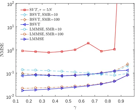
Fig. 4 depicts the performance of both algorithms when applied in identical scenarios and SNR= 20dB. Clearly, the optimized threshold and the Bayesian estimation step increase the performance of the proposed algorithm when accurate second order statistics are available. When the postulated statistics, i.e., those available to the operator are identical to the real statistics, the BSVT algorithm provides a better performance for all values of γ. The gain in performance is larger when the ratio of missing entries is smaller than 0.4. Interestingly, the boost in performance is substantial in the region in which SVT is least efficient when compared to the fundamental limit (See Fig. 3).
However, in practical scenarios the postulated and actual statistics are different. The impact of mismatched statistics is considered in the following section.
B. Robustness with respect to mismatched statistics
In order to address the problem of missing data recovery in a realistic scenario, a level of mismatch between the real covariance matrix and the one available to the operator is considered. The mismatch covariance matrix model presented in (27) is used in this section to assess the sensibility of the proposed algorithm to inaccurate prior knowledge. Hence, the LMMSE estimator and the BSVT algorithm are compared in the no-mismatch regime and for a SMR value of 100 and 10. The performance of the SVT-based recovery is included as a benchmark for comparing rank minimization based ap-proaches.
0 0.2 0.4 0.6 0.8 1 10-3
[image:9.612.320.557.62.256.2]10-2 10-1 100 101
Figure 5. LV data recovery performance using SVT, LMMSE estimation and BSVT for different levels of mismatch, when SNR= 10dB.
0.1 0.2 0.3 0.4 0.5 0.6 0.7 0.8 0.9 10-2
10-1 100 101 102
Figure 6. LV data recovery performance using SVT, LMMSE estimation and BSVT for different levels of mismatch, when SNR= 0dB.
with the LMMSE estimator, the performance of the BSVT algorithm does not change significantly when mismatch oc-curs. Moreover, the BSVT algorithm gives better recovery than the SVT-based recovery in all mismatch regimes throughout the range of γ. In comparison with the LMMSE estimation, the BSVT algorithm performs better for SMR = 100 when γ≤0.65. Furthermore, for SMR= 10the proposed approach is the best performing recovery method for almost all values of γ.
Fig. 5 depicts the performance of different estimation methods for different values of mismatch and SNR = 10 dB. Interestingly, the proposed approach outperforms SVT by almost an order of magnitude. Remarkably, the optimization of τ boosts the performance of the new algorithm in medium and low SNR regimes.
Fig. 6 shows the performance of SVT, BSVT and LMMSE for different values of mismatch in the low SNR regime
0 0.2 0.4 0.6 0.8 1
[image:9.612.55.296.63.256.2]10-6 10-5 10-4 10-3 10-2 10-1
Figure 7. LV data recovery performance using SVT, LMMSE estimation and BSVT for different levels of mismatch, when SNR= 50dB.
(SNR= 0 dB). Note that the case in which γ = 0.05 is not included in Fig. 6 because neither SVT nor BSVT converge to a low rank matrix in the experiments carried out for this paper. However, forγ≥0.15the new algorithm outperforms SVT by an order of magnitude.
A comparison between SVT, BSVT and LMMSE for dif-ferent values of mismatch is presented in Fig. 7 for a value of SNR= 50 dB. As expected, SVT outperforms BSVT in the noiseless case as in that case the problem in this paper boils down to the problem setting in [15]. It is worth noting that the fast degradation with respect to observation noise of SVT reported in [15] is also corroborated by the simulations in this work.
In practical scenarios, when the mismatch regime is difficult to establish, the choice between LMMSE and SVT is difficult to make. Interestingly, the impact of imperfect second order statistics for both LMMSE and BSVT is more significant in the high SNR regimes. However, BSVT is a robust alternative and gives better recovery in a wide range of missing data regimes.
C. Robustness with respect to different sampling patterns
The problem of recovering missing data when the subset of missing entries is not uniformly sampled is addressed in this section. In practical scenarios, a sensor failure or a downtime in the communication line provides the operator with a number of consecutive unavailable measurements in the state variable vectors. LetL0 be the number of consecutive missing entries.
The expected value ofL0varies depending on the reliability of
the sensing infrastructure. In the uniform sampling model this scenario is not possible. Therefore, a more general sampling procedure is introduced.
The proposed sampling model is based on a two-state Markov Chain. In this setting, for each entry (M)i,j of the
matrix M, the finite state machine depicted in Fig. 9, is
[image:9.612.56.295.309.500.2]0 0.2 0.4 0.6 0.8 1 10-3
[image:10.612.55.296.63.256.2]10-2 10-1
Figure 8. LV data recovery performance for the Markov-chain-based sampling model, using SVT and BSVT for different levels of mismatch, whenE[L0] = N and SNR= 20dB.
Figure 9. State diagram for the Markovian sampling model.
to the operator, or in state S2 in which case the entry is not
available. As before, the set Ω contains all the entries from the matrix M that are available to the operator. In Fig. 9,
p1 is the transition probability from state S1 toS2 andp2 is
the transition probability from S2 toS1. Hence, the expected
value of the ratio of missing entries is given by the steady state probability of being in S2. Consequently, the expected value
of the ratio of missing entries for the Markovian sampling model is
E[γ] = p1 p1+p2
. (39)
The expected number of consecutive missing entries, E[L0],
is:
E[L0] = n
X
l=0
l p1 p1+p2
(1−p2)l. (40)
Solving (40) for n→ ∞and combining with (39) leads to E[L0] =
1−E[γ] p2
2
(1−p2). (41)
Therefore, for any given γ and L0, using (39) and (41), p1
andp2are identified such that on average the sampling model
in Fig. 9 has a ratio of missing entries γ and the length of the vectors with consecutive missing entries L0. Note that
the case E[L0] = 1 reduces to the uniform sampling model
with probability P[(i, j)∈Ω] = 1−γ. In this framework, a comparison between the SVT and the BSVT-based recoveries is presented for the case in which the sampling pattern is not uniform. In order to consider the case in which a particular
0 20 40 60 80 100
0
20
40
60
80
100
Figure 10. Positions of the observed entries,Ω, generated by the Markovian model for a100×100matrix, whenE[L0] =NandE[γ] = 0.8.
feeder does not provide any measurements, the expected length of the vectors with missing data is selected to be equal to the length of the state variable vectors, i.e.,E[L0] =N. Fig.
[image:10.612.319.560.64.254.2]10 shows an example of a sampling pattern generated by the Markov-chain-based model, whenE[L0] =NandE[γ] = 0.8.
Fig. 8 compares the performance of the SVT-based recovery with the BSVT-based recovery for the case in which the matrix
Mis sampled using the Markov-chain-based sampling model
withE[L0] =N. Different levels of mismatch are introduced
to assess the robustness of the new algorithm to mismatched prior knowledge when the sampling pattern is not uniform. Remarkably, the performance of the proposed approach is not significantly affected by the amount of prior knowledge in any of the missing data regimes. Moreover, BSVT performs better than SVT when the sampling pattern is not uniform. A significant gain in performance is observed for small values of γ. Consider the following example for the sake of discussion, for a fixed tolerance of 10−2 in NMSE, the SVT algorithm
recovers up to 4% of the entries of the matrix M while
BSVT recovers 40% (See Fig. 8). The improvement in the data recovering performance for the same level of tolerance is significant. Numerical results in this section show that BSVT is not only providing better performance than SVT when the entries are not uniformly sampled but it is also robust to mismatched statistics. The robustness of the new algorithm extends to different sampling patterns. In view of this, BSVT represents a better alternative for recovering missing LV data in practical scenarios than SVT and LMMSE estimation.
D. Convergence analysis
[image:10.612.55.293.309.365.2]Table I
CONVERGENCE PERFORMANCE COMPARISON FOR THEUNIFORM SAMPLING CASE
SNR γ #Iters Time(s)
BSVT SVT BSVT SVT
0 0.15 2 51 17.32 68.24 0.85 4 30 32.06 53.62
10 0.15 4 191 52.38 111.59 0.85 2 32 6 19.54
20 0.15 2 365 15.89 169.92 0.85 2 92 13.8 84.17
50 0.15 18 485 271.47 100.42 0.85 2 145 8.67 69.16
Table II
CONVERGENCE PERFORMANCE COMPARISON FOR THEMARKOVIAN SAMPLING CASE
SNR γ #Iters Time(s)
BSVT SVT BSVT SVT
0 0.15 6 53 133.71 60.86 0.85 2 20 17.1 22.89
10 0.15 13 175 293.74 104.08 0.85 2 43 15.89 30.77
20 0.15 9 329 156.44 172.46 0.85 2 80 16.59 12.6
50 0.15 9 446 152.96 72.72 0.85 2 30 16.73 2.04
Table I shows a convergence performance comparison be-tween BSVT and SVT in terms of number of iterations and computational time for different SNR values and different values of γ. The computational platform used is the Iceberg HPC cluster at The University of Sheffield. The results are averaged over ten realizations ofΩ. The column #Iters shows the minimum number of iterations required by each algorithm to achieve the corresponding NMSE of Figs. 4, 5, 6 and 7. Time(s) denotes the time, measured in seconds, required to recover the missing entries in the matrix M for each case.
A similar comparison for the Markovian sampling case is presented in Table II. As expected, BSVT converges in fewer iterations but incurs a higher computational cost per iteration compared to SVT. Interestingly, the Markovian sampling case requires a larger number of iteration in most of the cases compared to the uniform sampling scenario. Moreover, BSVT requires less computation time in comparison to SVT in most of the cases for a large number of missing entries.
VII. CONCLUSION
A novel algorithm for recovering missing low voltage distribution systems data that admits a low rank description has been presented. The proposed approach, BSVT, combines
the low computational cost of SVT with the optimality of the LMMSE estimator when the data source is modelled as a mul-tivariate Gaussian random process and second order statistics are available. The combined new approach addresses the issues of individual recovery methods. The robustness of the new algorithm on both mismatched statistics and sampling patterns was demonstrated through simulations. In respect to the SVT algorithm the new approach addresses the issue of choosing the value of τ by calculating the optimal threshold at each iteration. Compared with the standard LMMSE estimator the new algorithm is robust to inaccurate second order statistics. In order to assess practical scenarios, a sampling model that incorporates missing state variable vectors, is illustrated. The performance gain compared to SVT was significant for both uniform and non-uniform sampling models. Ultimately, the proposed algorithm is shown to provide a robust and low complexity method to recover missing data in low voltage distribution systems.
REFERENCES
[1] A. Navarro-Espinosa and L. F Ochoa, “Probabilistic impact assessment of low carbon technologies in LV distribution systems,” IEEE Trans. Power Syst., vol. 31, no. 3, pp. 2192–2203, May 2016.
[2] R.A. Walling, R. Saint, R. C. Dugan, J. Burke, and L.A. Kojovic, “Summary of distributed resources impact on power delivery systems,” IEEE Trans. Power Del., vol. 23, no. 3, pp. 1636–1644, Jul. 2008. [3] C. Long and L. F. Ochoa, “Voltage control of PV-rich LV networks:
OLTC-fitted transformer and capacitor banks,”IEEE Trans. Power Syst., vol. 31, no. 5, pp. 4016–4025, Sep. 2016.
[4] M. Ozay, I. Esnaola, F. T. Y. Vural, S. R. Kulkarni, and H. V. Poor, “Sparse attack construction and state estimation in the smart grid: Centralized and distributed models,” IEEE Journal on Selected Areas in Communications, vol. 31, no. 7, pp. 1306–1318, Jul. 2013. [5] O. Kosut, L. Jia, R. J. Thomas, and L. Tong, “Malicious data attacks
on smart grid state estimation: Attack strategies and countermeasures,” in Proc. of the First IEEE International Conference on Smart Grid Communications, Oct. 2010, pp. 220–225.
[6] P. Gao, M. Wang, S. G. Ghiocel, J. H. Chow, B. Fardanesh, and G. Ste-fopoulos, “Missing data recovery by exploiting low-dimensionality in power system synchrophasor measurements,” IEEE Trans. Power Syst., vol. 31, no. 2, pp. 1006–1013, Mar. 2016.
[7] C. Genes, I. Esnaola, S. M. Perlaza, L. F. Ochoa, and D. Coca, “Re-covering missing data via matrix completion in electricity distribution systems,” in Proc. of the IEEE International Workshop on Signal Processing Advances in Wireless Communications, Jul. 2016, pp. 1–6. [8] Y. Isozaki, S. Yoshizawa, Y. Fujimoto, H.i Ishii, I. Ono, T. Onoda,
and Y. Hayashi, “Detection of cyber-attacks against voltage control in distribution power grids with PVs,”IEEE Trans. Smart Grid, vol. 7, no. 4, pp. 1824–1835, 2016.
[9] I. Esnaola, A. Tulino, and J. Garcia-Frias, “Linear analog coding of correlated multivariate Gaussian sources,” IEEE Trans. Commun., vol. 61, no. 8, pp. 3438–3447, Aug. 2013.
[10] E. J. Cand`es and B. Recht, “Exact matrix completion via convex optimization,”Communications of the ACM, vol. 55, no. 6, pp. 111–119, 2012.
[11] E. J. Cand`es and T. Tao, “The power of convex relaxation: Near-optimal matrix completion,”IEEE Trans. Inf. Theory, vol. 56, no. 5, pp. 2053– 2080, May 2010.
[12] E. J. Cand`es and Y. Plan, “Matrix completion with noise,”Proceedings of the IEEE, vol. 98, no. 6, pp. 925–936, Jun. 2010.
[13] R. Meka, P. Jain, and Inderjit S. D., “Matrix completion from power-law distributed samples,” in Proc. of the Advances in Neural Information Processing Systems 22, Dec. 2009, pp. 1258–1266.
[14] V. Kekatos, Y. Zhang, and G. B. Giannakis, “Electricity market forecasting via low-rank multi-kernel learning,” IEEE J. Sel. Topics Signal Process., vol. 8, no. 6, pp. 1182–1193, Dec. 2014.
[16] E. J. Cand`es, C. A. Sing-Long, and J. D. Trzasko, “Unbiased risk estimates for singular value thresholding and spectral estimators,”IEEE Trans. Signal Process., vol. 61, no. 19, pp. 4643–4657, Oct. 2013. [17] C. M. Stein, “Estimation of the mean of a multivariate normal
distribution,” The Annals of Statistics, pp. 1135–1151, Nov. 1981. [18] Electricity North West Limited, “Low voltage network solutions,”
[Online]. Available: http://www.enwl.co.uk/lvns.
[19] G. A. Seber, A matrix handbook for statisticians, vol. 15, John Wiley & Sons, 2008.
[20] R. Meka, P. Jain, and I. S. Dhillon, “Matrix completion from power-law distributed samples,” inProc. of the Advances in neural information processing systems, Dec. 2009, pp. 1258–1266.
[21] T. Cover and J. Thomas, Elements of information theory, John Wiley & Sons, 2012.
[22] A. Kolmogorov, “On the Shannon theory of information transmission in the case of continuous signals,” IRE Transactions on Information Theory, vol. 2, no. 4, pp. 102–108, Dec. 1956.
[23] J.F. Sturm, “Using SeDuMi 1.02, a MATLAB toolbox for optimization over symmetric cones,”Optimization Methods & Software, vol. 11, no. 1-4, pp. 625–653, 1999.
[24] K.C. Toh, M.J. Todd, and R.H. Tutuncu, “SDPT3 - A MATLAB software package for semidefinite programming, version 1.3,” Optimization Methods & Software, vol. 11, no. 1-4, pp. 545–581, 1999.
[25] Z. Liu and L. Vandenberghe, “Interior-point method for nuclear norm approximation with application to system identification,” SIAM Journal on Matrix Analysis and Applications, vol. 31, no. 3, pp. 1235–1256, Nov. 2009.
[26] D. Donoho and M. Gavish, “Minimax risk of matrix denoising by singular value thresholding,” Ann. Statist., vol. 42, no. 6, pp. 2413– 2440, Dec. 2014.
[27] X. Jia, X. Feng, and W. Wang, “Rank constrained nuclear norm minimization with application to image denoising,” Signal Processing, vol. 129, pp. 1–11, Dec. 2016.
[28] I. Esnaola, A. M. Tulino, and H. V. Poor, “Mismatched MMSE estimation of multivariate Gaussian sources,” in Proc. of the IEEE International Symposium on Information Theory, Jul. 2012, pp. 716– 720.

![Figure 8. LV data recovery performance for the Markov-chain-based samplingmodel, using SVT and BSVT for different levels of mismatch, whenN E[L0] = and SNR = 20 dB.](https://thumb-us.123doks.com/thumbv2/123dok_us/1968773.157927/10.612.319.560.64.254/figure-recovery-performance-markov-samplingmodel-different-levels-mismatch.webp)
