This is a repository copy of
A Gaussian process regression for natural gas consumption
prediction based on time series data
.
White Rose Research Online URL for this paper:
http://eprints.whiterose.ac.uk/136105/
Version: Accepted Version
Proceedings Paper:
Laib, O., Khadir, M.T. and Mihaylova, L.S. orcid.org/0000-0001-5856-2223 (2018) A
Gaussian process regression for natural gas consumption prediction based on time series
data. In: 2018 21st International Conference on Information Fusion (FUSION). 2018 21st
International Conference on Information Fusion (FUSION) , 10-13 Jul 2018, Cambridge,
UK. IEEE , pp. 55-61. ISBN 978-0-9964527-6-2
10.23919/ICIF.2018.8455447
© 2018 ISIF. Personal use of this material is permitted. Permission from IEEE must be
obtained for all other users, including reprinting/ republishing this material for advertising or
promotional purposes, creating new collective works for resale or redistribution to servers
or lists, or reuse of any copyrighted components of this work in other works. Reproduced
in accordance with the publisher's self-archiving policy.
eprints@whiterose.ac.uk https://eprints.whiterose.ac.uk/
Reuse
Items deposited in White Rose Research Online are protected by copyright, with all rights reserved unless indicated otherwise. They may be downloaded and/or printed for private study, or other acts as permitted by national copyright laws. The publisher or other rights holders may allow further reproduction and re-use of the full text version. This is indicated by the licence information on the White Rose Research Online record for the item.
Takedown
If you consider content in White Rose Research Online to be in breach of UK law, please notify us by
A Gaussian Process Regression for Natural Gas
Consumption Prediction Based on Time Series Data
Oussama Laib
∗, Mohamed Tarek Khadir
∗and Lyudmila Mihaylova
∗∗∗Dep. of Computer Science (LabGED) University of Badji Mokhtar Annaba (UBMA), Annaba, Algeria
laib@labged.net, khadir@labged.net
∗∗Dep. of Automatic Control and Systems Engineering (ACSE) University of Sheffield, Sheffield, UK
l.s.mihaylova@sheffield.ac.uk
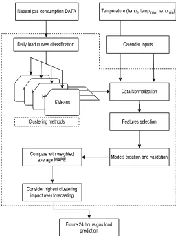
Abstract—For several economical, financial and operational reasons, forecasting energy demand becomes a key instrument in energy system management. This paper develops a natural gas forecasting approach, which consists of two major phases: 1) it classifies the natural gas consumption daily pattern sequences into different groups with similar attributes. 2) the design and training of multiple autoregressive Gaussian Process models phase is carried out using the Algerian natural gas market data together with exogenous inputs consisting in weather (tempera-ture) and calendar (day of the week, hour indicator) factors. The main novelty in this work consists of the investigation of multiple different clustering techniques for better analysis and clustering of natural gas consumption data. The impact of the obtained clusters, by each technique, is then summarized and evaluated with respect to the prediction accuracy.
Index Terms—time series classification, gaussian process, load forecasting, natural gas consumption
I. INTRODUCTION
The development of energy modeling for short term fore-casting of the patterns such as periodicity or seasonality on the energy demand can leads to significant saving especially on dispatch scheduling and maintenance planning. Subse-quently, this development became extremely important since it stimulates analysts, economists and other experts to use computational intelligence techniques as a supporting tool for decision making in order to increase the efficiency in the energy distribution.
Natural gas is a primary energy source in Algeria where its demand fluctuates over time. Furthermore, it is difficult to predict the demand, due to the variations and non-stationarity of the load series. Other factors that have an influence on the gas consumption are the thermal energy that is depleted for heating of residential areas, for generating electricity and for the industrial sector.
The variety of customer profiles, the high dependence on seasonal and climate aspects, together with the actual gas consumption limit the maximum accuracy that classical single model prediction approaches [1] can provide. To overcome this limitation there are techniques that rely on multiple models. Multiple models are often combined with the divide-and-conquer approaches for solving such complex problems [2].
The literature is rich with forecasting approaches for natural gas and energy consumption forecasting in a short term. Some
of the most widely used methods which have been success-fully applied are: artificial neural networks [3] and a long short-term memory (LSTM) recurrent neural network (RNN) for electrical load forecasting. In [4], neural networks with multilayer perceptrons are proposed, to forecast the natural gas consumption in Szczecin, Poland. Fuzzy approaches are proposed in [5] [6] and autoregressive integrated moving average (ARIMA) algorithms in [7].
However, another nonparametric machine learning method for regression, the Gaussian process regression has been successfully applied to many different areas such as electricity forecasting [8] [9], wind power forecasting [10] and ground-water level time-series forecasting [11].
This paper investigates several divided-and-conquer ap-proaches for the purposing of forecasting the natural gas consumption. Inspired from [12], This approach is based on splitting the Algerian natural gas hourly consumption of 2014 into multiple subsets using different kinds of clustering methods. The dataset division is made by regrouping the daily pattern sequence of the 24 hours load using three powerful methods. After the division process, multiple local auto-regressive Gaussian Process (AR-GP) models are developed for a specific variation of similar daily curves according to each clustering method. Finally, the results obtained by several non-supervised classifiers are compared over the problem for load consumption prediction.
The rest of this paper is organized as follows: Section II presents data for the case study, Section III introduces the proposed methodology upon which the paper is based on, Section IV provides a brief overview of the theory of Auto-Regressive Gaussian Process, Section V shows and analyses the results of the experiment for natural gas load forecasting. Finally, conclusion and discussion are summarized in Section VI.
II. DATA DESCRIPTION
This study is based on the Algerian natural gas consumption for both residential and industrial sectors data and a corre-sponding weather data recorded by a meteorological service company.
SONELGAS for the year of 2014. Fig. 1 shows fluctuation in gas consumption through the entire observed year along with temperature. Besides, there are many other exogenous factors that could be used for this type of forecasting like weather factors (wind speed, humidity, nebulosity) and cal-endar information (day of the week, is a holiday day, season) [13]. There are various factors which may influence the rate of natural gas consumption. These include : oil prices, number of clients, GDP, natural gas price, etc [14]. However, for a daily or hourly based forecasting horizon, this kind of data does not have any impact on the outcome of the short term consumption like in the current research.
2014-01 2014-03 2014-05 2014-07 2014-09 2014-11 2015-01
0.2 0.4 0.6 0.8 1.0
Temperature
Temperature
0.2 0.4 0.6 0.8 1.0
Consommation
[image:3.612.49.300.206.347.2]Consommation
Fig. 1: Hourly recorder natural gas consumption and temper-ature during 2014.
III. DAILY LOAD CURVES CLASSIFICATION
The first step of the proposed approach is to classify samples
of historical segments H2014
D0. . . D364
into K clusters
containing identical daily load curves, where each historical
segment (day x) is represented in 24 hours consumption
vector Dx = {C0, C1...C23} with Ch is the consumption at
a specific hour h. As the numberK is unknown in this case,
from a statistical point of view this issue is considered as an unsupervised curves classification problem. To group the daily consumption curves, different techniques are applied.
A. K-Means
First, a centroid based KMeans is used, but with the need of
evaluating theKwe suppose that there is a daily consumption
and meteorological variables correspondence. Therefore, we assume that K could be equal to 3 (winter, summer, and spring-autumn) clusters.
B. HDBSCAN
Secondly, a hierarchical density-based clustering method is used. The current method was firstly introduced by Campello et. al in [15] and [16], where it improves the DBSCAN method by transforming it into a hierarchical clustering algorithm. Thus, it generates a complete density-based clustering hierar-chy from which a simplified hierarhierar-chy composed only of the most significant clusters can be easily extracted. This method requires only one parameter which represents the minimum size of the cluster.
C. MOHGP
Another non-parametric clustering method is used, but unlike the HDBSCAN the mixture of hierarchical Gaussian Process is specialized on structural time series. MOHGP is proposed by James Hensman in [17] which is a combination of two Bayesian non-parametric algorithms, where it combines Gaussian processes (GPs) approach to model time-series and Dirichlet processes (DPs) to perform clustering.
D. Mixture of K-means and HDBSCAN
The last clustering technique is a result of two combined methods (HDBSCAN and KMeans): where it keeps the 3 clusters obtained by the KMeans and add another two clusters which get recognized by the HDBSCAN. There is a significant difference between the obtained clustering results. The reason is due to the fact that these clusters represents two different time periods in of the year: the first is the period of the Ramadan and the second one is the period of national and religious holidays. During these holiday periods the consump-tion patterns are unique.
IV. GAUSSIANPROCESSREGRESSION METHOD FOR
TIME-SERIES MODELING:
Once daily curves are regrouped, an AR-GP model is trained to learn the data for each cluster. Hence, every model handles the forecasting task for all hourly load in the corresponding
cluster. By each GP model a single value Ct is predicted
depending essentially on the following inputs: First, the
previ-ous lagged observationsCt−1, Ct−24, Ct−168which represent
the consumption of the previous hour, the same hour of the previous day and the same hour of the previous week. Then,
meteorological factors corresponding to the temperature Tt,
the maximum Tmax and the minimum Tmin temperature of
the day are considered.
Fig. 3 presents the computation procedure for the proposed gas demand prediction method.
Gaussian Process models are considered as a collection of
random variables that predictCtat timetfor a given inputxt.
Assume thatf is a latent function, which provides the values
for each data point according to:
Ct=f(t) +α (1)
whereα∼N(0;σ2
)is a Gaussian noise with a zero mean and
a varianceσ2
. Noting that a Bayesian inference is performed
and hence the posterior predictive distribution of f can be
written as follows:
f(x)∼GP(m(x), k(x, x′)) (2)
wheref(x)is the real process to model, xandx′ are two
different points. Herem(x)is the mean value which is equal to
zero in this case andk(x, x′)is the kernel function. Because of
the dependence of the performance of the GPs on the chosen kernel, a radial basis function (RBF) kernel is adopted, also known as the squared exponential. The RBF kernel is given by:
k(x, x′) = exp
−1 2d
x
l, x′
l
2
00:00
04-Mar 03:00 06:00 09:00Time, hours12:00 15:00 18:00 21:00 0.2
0.4 0.6 0.8
Mean load
cluster 1 cluster 2 cluster 3
(a) KMeans result
00:00
04-Mar 03:00 06:00 09:00Time, hours12:00 15:00 18:00 21:00 0.2
0.4 0.6 0.8
Mean load
cluster 1 cluster 2 cluster 3 cluster 4 cluster 5
(b) HMOGP result
00:00
04-Mar 03:00 06:00 09:00 12:00 15:00 18:00 21:00
Time, hours
0.2 0.4 0.6 0.8
Mean load
cluster 1 cluster 2 cluster 3 cluster 4 cluster 5
(c) Mixed of KMeans and HDBCAN result
00:00
04-Mar 03:00 06:00 09:00 12:00 15:00 18:00 21:00
Time, hours
0.2 0.4 0.6 0.8
Mean load
cluster 1 cluster 2 cluster 3 cluster 4 cluster 5 cluster 6
[image:4.612.356.524.47.239.2](d) HDBSCAN result
Fig. 2: Average load for clusters obtained by each method.
Fig. 3: Main steps of the proposed framework.
The radial basis function provides an expressive kernel to
model smooth functions. The hyper-parameters l (called the
length-scale) can be varied to increase or reduce the correlation
between points and consequentially the smoothness of the resulting function.
Depending on the hyper-parameters of the kernel function, predictions are correlated with already observed values that have been recently observed. However, the influence of dif-ferent variables on gas consumption is defined by the hyper-parameters of the covariance function which can be derived by maximizing the marginal likelihood. The log-marginal likelihood (LML) is defined as:
log(p|X, θ) =−1
2CTk−1C−
1
2log|K| −
n
2log2π (4)
where the first term is the data-fit, the second term is a complexity penalty and the last term is a normalizing constant
withnbeing the number of training samples.
The dataset is separated then into two partitions, the first partition (70 % ) is for the fitting and optimizing of the GP’s hyper-parameters, the rest (30 %) is for the test to evaluate the model quality.
In order to achieve a better estimation of hyper-parameters of covariance functions, using an appropriate approach to normalize the time series data is critical before feeding it to the GP model. The outputs and inputs data are normalized to
an interval between [0, 1]. Hence, a value ofX is normalized
toX′ by computing:
X′= X
Xmax
(5)
whereX′ is the new value, X is the old value and Xmax is
the largest consumption value in the year.
V. EXPERIMENTAL RESULTS A. Clustering
[image:4.612.45.301.289.631.2]methods. At the end of the clustering, 365 daily curves of
in the dataset H2014 are all labeled with its correspondent
cluster Kx.
H2014
" D0[C0...C23] Kx
..
. ...
D364[C0...C23] Kx
[image:5.612.311.565.73.357.2]#
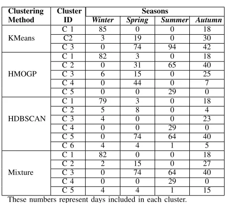
TABLE I: Season’s day count per cluster
Clustering Cluster Seasons
Method ID Winter Spring Summer Autumn
C 1 85 0 0 18
KMeans C2 3 19 0 30
C 3 0 74 94 42
C 1 82 3 0 18
C 2 0 31 65 40
HMOGP C 3 6 15 0 25
C 4 0 44 0 7
C 5 0 0 29 0
C 1 79 3 0 18
C 2 5 8 0 4
HDBSCAN C 3 4 0 0 23
C 4 0 0 29 0
C 5 0 74 64 40
C 6 4 4 1 5
C 1 82 0 0 18
C 2 2 15 0 27
Mixture C 3 0 74 64 40
C 4 0 0 29 0
C 5 4 4 1 15
These numbers represent days included in each cluster.
In order to be able to compare results obtained in each clustering method in Table. I, the clusters are related to a season which represented the most number of days, this is determined by the seasons of the year. The comparison of results is therefore based on the labeled seasons.
B. Features selection
The most appropriate features must be determined in order to enhance the prediction accuracy. The investigation started using only 3-dimensional input vector containing the historical
load (Ct−1, Ct−24, Ct−168). Furthermore, other features were
added sequentially as indicated in Table. II to observe its impact on estimating one hour ahead.
To measure the error in estimated loads, the models are eval-uated based on the Mean Absolute Percentage Error calculated according to the following formula:
M AP E=100%
N
N
X
i=1
Ai−Pi
Ai
(6)
[image:5.612.101.249.100.144.2]Because of the complexity of the load time series, the experiments show that every time the AR-GP injected with exogenous variables, it provides a significantly better fore-casting results. The correlation of natural gas consumption with temperature is -0.70 which means that there is no strong relevance between the two variations. However, adding the temperature variables reduced the MAPE in all clusters especially in the winter period. The unexpected improvement
TABLE II: Mean Absolute Percentage Error according to features combination
Experiments Exp 1 Exp 2 Exp 3 Exp 4 Exp 5 Exp 6 Historical
Inputs
x x x x x x
Temp x x x
Day Ind x x
Hour Ind x x x
Kmeans method
C1 MAPE 3.48 3.89 3.55 2.41 2.25 2.05
C2 MAPE 4.54 4.94 4.39 3.16 2.90 2.68 C3 MAPE 7.64 6.18 7.31 5.79 5.88 4.84
HDBSAN method
C1 MAPE 5.16 4.93 4.81 4.27 3.01 3.10 C2 MAPE 6.24 4.68 4.54 2.94 2.66 3.28
C3 MAPE 8.29 6.00 6.08 5.49 4.06 4.00
C4 MAPE 7.91 6.60 7.43 6.94 6.24 5.78
C5 MAPE 8.25 5.68 6.09 6.42 3.57 4.23
C6 MAPE 10.12 7.83 18.34 10.02 3.48 1.59
HMOGP method
C1 MAPE 5.26 5.13 4.87 4.37 3.41 3.21
C2 MAPE 8.35 5.89 7.63 5.90 3.96 3.58
C3 MAPE 6.45 4.38 5.40 4.72 4.07 4.20 C4 MAPE 8.68 7.70 8.19 7.44 6.84 6.23 C5 MAPE 8.25 5.68 6.09 6.42 3.57 4.23
Mixed method
C1 MAPE 5.16 4.93 4.81 4.27 3.37 3.07
C2 MAPE 8.76 5.37 5.66 6.15 3.92 3.51 C3 MAPE 7.99 6.68 7.50 7.03 6.32 5.70
C4 MAPE 8.25 5.68 6.09 6.42 3.57 4.23
C5 MAPE 10.12 7.83 18.34 10.02 3.48 1.59
is also in the summer period which leads to the fact of the AR-GP is not influenced by the temperature as an indicating value for hotness or coldness but influenced by value that indicates the period in the day which corresponds the load.
monday thursday wedensday tuesday friday saturday sunday
0.88 0.90 0.92 0.94 0.96 0.98 1.00
Average Load
Fig. 4: The daily average natural gas consumption per week.
Apart from using historical and exogenous attributes, the experiments also involved two different kinds of calendar variations. The first is a daily indicator, to identify the day of the week which related to the predicted load. Identifying the day for which forecast is performed can help the model to distinguish between working days and holidays and also to recognize the first day of the week from the last ones. Fig. 4 shows the variety of daily average load per week on the generated clusters. The second calendar inputs is an hourly indicator which is considered as a very strong intraday periodic pattern.
[image:5.612.59.289.171.376.2] [image:5.612.312.561.437.537.2]validation data is not straightforward. There are two main causes that occur the inconsistency of the model’s performance through training and testing sets: the first cause is when the influence of an exogenous factor doesn’t cover the entire period of the correspondent cluster, like in the case of KMeans clusters: C2 and C3, the best input combination is (Exp 5) because the error during test is lower than in (Exp 6) 4.5%, 4.2% respectively. The hyper-parameters of the kernel are optimized during the fitting of the AR-GPR by maximizing the LML. As the LML have a multiple local optima, this means that the model may fall in the over-fitting phenomena, which is the second cause that makes the covariance function will tend to have a poor predictive performance on the test unlike on training where is it the case in (Exp 6) with HDBSCAN C5, the MAP-Errors in training and test are (1.59% and 395.72% respectively) thus, the feature combination in (Exp 6) will be ignored.
C. Load forecasting results
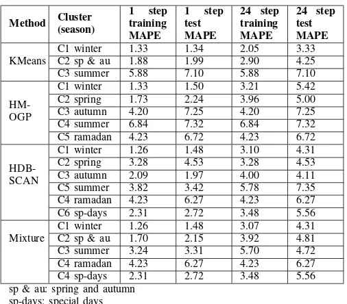
After selecting the most convenient features, Table. III reports the mean absolute percentage error for AR-GP based on the proposed clustering methods.
Injecting predicted load in every iteration is the main concept for the stepwise forecasting. Furthermore, AR-GP models are extremely sensitive to the historical consumption, thus, a non-accurate estimation will definitely lead to a very bad performance along the rest of the 24 hours ahead, and this is the case when the AR-GP model is constructed basing
on a load prior to the desired one (Ct−1). Meanwhile, we
should note that under some circumstances an AR-GP regress according to the prior load could distort its performance. Therefore, the previous load will not be used in the forecasting process. Table. III obviously expresses seven cases where the prior load is ignored (C3), (C3, C4, C5), (C2, C4) and (C4) in KMeans, HMOGP, HDBSCAN and Mixture clusters respectively. Consequently, the 1 step forecasting error will be exactly the same as the 24 steps forecasting error.
Each cluster deserved a particular consideration, and Be-cause of the high distinction in the generated daily load curves by each clustering approach, there is no general indication of how effective a daily load curves classification procedure can be given without applying a relevant comparative evaluation.
The weighted arithmetic mean is applied instead of the ordinary mean to calculate an average MAPE that represents the error for a clustering method.
M AP E= 1
N
N
X
i=1 P4
j=1wjM AP Ei
P4
j=1wj
!
(7)
Equation (7) expresses the weighted average of the mean
absolute error (M AP E), where wj is the number of days
per seasonj (winter, spring, summer and autumn) counted in
each cluster i.
[image:6.612.312.565.73.295.2]A summarized comparison between actual and forecast gas consumption in terms of mean absolute percentage error shown in Table. IV. The results indicate that the AR-GP
TABLE III: Forecasting MAPE based on the clustering ap-proaches
Method Cluster (season)
1 step training MAPE
1 step test MAPE
24 step training MAPE
24 step test MAPE
C1 winter 1.33 1.34 2.05 3.33 KMeans C2 sp & au 1.88 1.99 2.90 4.25 C3 summer 5.88 7.10 5.88 7.10
HM-OGP
C1 winter 1.33 1.50 3.21 5.42 C2 spring 1.73 2.24 3.96 5.00 C3 autumn 4.20 7.25 4.20 7.25 C4 summer 6.84 7.32 6.84 7.32 C5 ramadan 4.23 6.72 4.23 6.72
HDB-SCAN
C1 winter 1.26 1.48 3.10 4.31 C2 spring 3.28 4.53 3.28 4.53 C3 autumn 2.09 1.97 4.00 4.11 C5 summer 3.82 3.42 5.78 7.35 C4 ramadan 4.23 6.27 4.23 6.27 C6 sp-days 2.31 2.72 3.48 5.56 C1 winter 1.26 1.48 3.07 4.31 Mixture C2 sp & au 1.70 2.15 3.92 4.81 C3 summer 3.24 3.31 5.70 4.72 C4 ramadan 4.23 6.27 4.23 6.27 C4 sp-days 2.31 2.72 3.48 5.56 sp & au: spring and autumn
sp-days: special days
performs much better on the Mixture method amongst all other clustering methods on the test period. The reason of choosing the Mixture method is because of the performance stability of AR-GP through training and testing sets compared to its performance on KMeans, HMOPG and HDBSCAN clusters.
Additionally, theM AP Eobtained of Mixture method clusters
on test is 4.77%, which is an improvement over the KMeans, HMOPG and HDBSCAN by 16.53%,19.83% and 25.91% respectively.
The results of the forecasts for gas demand for the Algerian market reported with the use of Mixture clustering method clusters are illustrated in Figures. 5, 6, 7, 8 and 9. The labeled figures (a) and (b) presented the results through learning and test period respectively.
00:00
12-Jan 03:00 06:00 09:00 12:00 15:00 18:00 21:00 Time, hours
0.25 0.30 0.35 0.40
Normalized load
Actual load 24 steps forecasting 1 step forecasting
(a)
00:00
24-Dec 03:00 06:00 09:00 12:00 15:00 18:00 21:00 Time, hours
0.30 0.35
Normalized load
Actual load 24 steps forecastint 1 step forecasting
(b)
[image:6.612.323.556.501.673.2]00:00
23-Mar 03:00 06:00 09:00 12:00 15:00 18:00 21:00 Time, hours
0.20 0.25 0.30
Normalized load
Actual load 24 steps forecasting 1 step forecasting
(a)
00:00
30-Nov 03:00 06:00 09:00 12:00 15:00 18:00 21:00 Time, hours
0.175 0.200 0.225 0.250 0.275
Normalized load
Actual load 24 steps forecastint 1 step forecasting
[image:7.612.325.553.49.221.2](b)
Fig. 6: 24 hour forecast through training and testing Spring and Autumn period
00:00
10-Feb 03:00 06:00 09:00 12:00 15:00 18:00 21:00 Time, hours
0.25 0.30 0.35 0.40 0.45
Normalized load
Actual load 24 steps forecasting 1 step forecasting
(a)
00:00
10-Nov 03:00 06:00 09:00Time, hours12:00 15:00 18:00 21:00 0.20
0.25 0.30
Normalized load
Actual load 24 steps forecastint 1 step forecasting
[image:7.612.64.291.52.227.2](b)
Fig. 7: 24 hour forecast through training and testing special days period
00:00
10-Apr 03:00 06:00 09:00Time, hours12:00 15:00 18:00 21:00 0.100
0.125 0.150 0.175
Normalized load
Actual load 24 steps forecasting 1 step forecasting
(a)
00:00
21-Oct 03:00 06:00 09:00Time, hours12:00 15:00 18:00 21:00 0.06
0.08 0.10 0.12
Normalized load
Actual load 24 steps forecastint 1 step forecasting
(b)
Fig. 8: 24 hour forecast through training and testing summer period
00:00
03-Jul 03:00 06:00 09:00Time, hours12:00 15:00 18:00 21:00 0.05
0.10 0.15
Normalized load
Actual load 24 steps forecasting 1 step forecasting
(a)
00:00 27-Jul 03:00 06:00 09:00 12:00 15:00 18:00 21:00
Time, hours 0.05
0.08 0.10 0.12 0.15
Normalized load
Actual load 24 steps forecastint 1 step forecasting
[image:7.612.63.293.280.452.2](b)
Fig. 9: 24 hour forecast through training and testing ramadan period
TABLE IV: M AP E based on the clustering approaches
Approach TrainMAP E TestMAP E
KMeans 4.37% 5.63%
HMOGP 4.20% 5.82%
HDBSCAN 4.58% 6.19%
Mixture 4.56% 4.77%
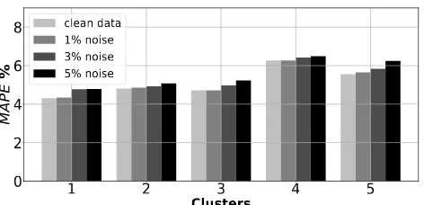
As a test-bench experiment, a noise can be added to the inputs to cover different kinds of uncertainties in the measurement. Three levels of simulated random noise were added to inputs vectors: 1%, 3% and 5%. Because of the prior data normalization from [0,1], the inputs noise values was randomly generated from -0.01, -0.03 and -0.05 to 0.01, 0.03 and 0.05 respectively according the noise percentage. Occurring prediction with this uncertainties should definitely
lead to an increase in the M AP E. Unexpectedly, AR-GPs
models show a very powerful ability of handling the noisy inputs, where even 5% added noise did not inadequately effect the prediction accuracy and results error increasing by 8% only and barely increases after 1% of noise is added. Fig. 10
illustrates theM AP Eincrease with regard to the noise level.
1 2 3 4 5
Clusters
0 2 4 6 8
M
A
PE
%
clean data 1% noise 3% noise 5% noise
[image:7.612.63.293.506.678.2] [image:7.612.318.554.559.673.2]TABLE V: Models and Months
Model Name Data Months
Model 1 January, February
Model 2 March
Model 3 April
Model 4 June, July Model 5 August, September, October Model 6 November, December
To evaluate the results obtained by the proposed approach, a comparison with another two divide-and-conquer approaches are conducted. The first method was developed in [18] is considered in the preliminary analysis for energy forecasting, where the dataset is split according to the holiday (i.e., Friday, Saturday and other holidays), to working days, to pre-holidays and to special days.
A second proposed by Mustafa Akpinar in [19], the data is split into six monthly subsets shown in Table. V.
TABLE VI: Average prediction M AP E for every cluster
according to each approach
Cluster TrainingM AP E% TestM AP E%
MIX APP1 APP2 MIX APP1 APP2 Cluster 1 3.92 5.08 4.76 4.31 7.82 6.18 Cluster 2 3.92 4.83 8.63 4.81 6.16 10.68 Cluster 3 5.70 2.72 4.03 4.72 5.56 9.87 Cluster 4 4.23 5.65 10.09 6.27 4.90 11.48 Cluster 5 3.48 / 6.91 5.56 / 6.50
Cluster 6 / / 5.72 / / 5.60
Average 4.56 5.25 6.95 4.77 5.96 8.13 MIX: prediction based on Mixture clustering method.
APP1, APP2: prediction based on first and second benchmark approaches.
From comparison results shown in Table. VI, it can be noticed that the proposed method gives a very accurate fore-cast for practical needs even when compared with the two benchmark methods.
VI. CONCLUSION
This paper investigates the practical aspects of development of forecasting the Algerian natural gas consumption. There is a strong correlation of the natural gas load with meteorological elements which is mainly represented by temperature for the residential sector and physical and statistical factors like season of the year, day of the week for the industrial sector. Load data of 2014 is analyzed and clustered using different clustering methods in order to classify daily load profiles according to the similarity measures of each clustering method. Based on the grouped daily load curves and using tem-perature with calendar inputs, multiple models construction are conducted by several experiments to determine the most influential factor. Forecasting results of 2014 are summarized and expressed in mean absolute percentage error. The average
calculatedM AP E on training and test datasets is 4.56% and
4.77%, which was achieved using mixture of KMeans and HDBSCAN method.
Classifying load curves into a huge amount of groups or adopting many different models does not necessarily improve the forecasting results, even in the case of using powerful clustering techniques. Contrarily, properly segmented and clas-sified clusters can enhance the overall quality of the developed models considerably.
REFERENCES
[1] P. Potoˇcnik, E. Govekar, and I. Grabec, “Building forecasting applica-tions for natural gas market,” inNatural gas research progress, N. David and T. Michel, Eds. New York: Nova Science Publishers, 2008, pp. 505–530.
[2] P. Potoˇcnik and E. Govekar, “Practical results of forecasting for the natural gas market,” inNatural Gas. New York: Sciyo, 2010, ch. 16, pp. 371–392.
[3] W. Kong, Z. Y. Dong, Y. Jia, D. J. Hill, Y. Xu, and Y. Zhang, “Short-term residential load forecasting based on lstm recurrent neural network,”
IEEE Transactions on Smart Grid, Sep. 2017.
[4] J. Szoplik, “Forecasting of natural gas consumption with artificial neural networks,”Energy, vol. 85, pp. 208–220, jun 2015.
[5] G. Cerne, D. Dovzan, and I. Skrjanc, “Short-term load forecasting by separating daily profile and using a single fuzzy model across the entire domain,”IEEE Transactions on Industrial Electronics, 2018.
[6] D. M. Minhas, R. R. Khalid, and G. Frey, “Short term load forecasting using hybrid adaptive fuzzy neural system: The performance evaluation,”
in2017 IEEE PES PowerAfrica. IEEE, jun 2017.
[7] L. Friedrich and A. Afshari, “Short-term forecasting of the abu dhabi electricity load using multiple weather variables,” Energy Procedia, vol. 75, pp. 3014–3026, aug 2015.
[8] J. Lourenco and P. Santos, “Short term load forecasting using gaussian process models,” Systems Engineering and Computers, INESC - Coim-bra, Tech. Rep. 5, Jun. 2010.
[9] M. Alamaniotis, S. Chatzidakis, and L. Tsoukalas, “Monthly load fore-casting using kernel based gaussian process regression,” inMedPower 2014. Institution of Engineering and Technology, 2014.
[10] N. Chen, Z. Qian, X. Meng, and I. T. Nabney, “Short-term wind power fore- casting using gaussian processes,” in International Joint
Conference on Artificial Intelligence (IJCAI’13), Beijing, China, Aug.
2013.
[11] N. S. Raghavendra and P. C. Deka,Multistep Ahead Groundwater Level
Time-Series Forecasting Using Gaussian Process Regression and ANFIS.
New Delhi: Springer India, 2016, pp. 289–302.
[12] K. E. Farfar and M. T. Khadir, “A two-stage short-term load forecasting approach using temperature daily profiles estimation,”Neural
Comput-ing and Applications, jan 2018.
[13] D. Sebalj, J. Mesaric, and D. Dujak, “Predicting natural gas consumption a literature review,” in28th Central European Conference on Information
and Intelligent Systems (CECIIS ’17), Varadin, Croatia, Sep. 2017, pp.
293–300.
[14] B. Soldo, “Forecasting natural gas consumption,” Applied Energy, vol. 92, pp. 26–37, apr 2012.
[15] R. J. G. B. Campello, D. Moulavi, and J. Sander, “Density-based clus-tering based on hierarchical density estimates,” inKnowledge Discovery
and Data Mining (PAKDD’13). Springer Berlin Heidelberg, Apr. 2013,
p. 160172.
[16] J. Hensman, N. D. Lawrence, and M. Rattray, “Hierarchical bayesian modelling of gene expression time series across irregularly sampled replicates and clusters,” BMC Bioinformatics, vol. 14, no. 1, p. 252, 2013.
[17] R. J. G. B. Campello, D. Moulavi, A. Zimek, and J. Sander, “Hierar-chical density estimates for data clustering, visualization, and outlier detection,” ACM Transactions on Knowledge Discovery from Data, vol. 10, no. 1, pp. 1–51, jul 2015.
[18] A. Franco and F. Fantozzi, “Analysis and clustering of natural gas con-sumption data for thermal energy use forecasting,”Journal of Physics:
Conference Series, vol. 655, pp. 1–10, nov 2015.
[19] M. Akpinar and N. Yumusak, “Forecasting household natural gas consumption with arima model: A case study of removing cycle,” in
2013 7th International Conference on Application of Information and
[image:8.612.48.313.318.410.2]