Nonlinear modal analysis via non-parametric machine learning tools

This is a repository copy of Nonlinear modal analysis via non-parametric machine learning tools.

White Rose Research Online URL for this paper: http://eprints.whiterose.ac.uk/135608/

Version: Accepted Version

Article:

Dervilis, N. orcid.org/0000-0002-5712-7323, Simpson, T.E., Wagg, D. et al. (1 more

author) (2018) Nonlinear modal analysis via non-parametric machine learning tools. Strain. ISSN 0039-2103

https://doi.org/10.1111/str.12297

This is the peer reviewed version of the following article: Dervilis N, Simpson TE, Wagg DJ, Worden K. Nonlinear modal analysis via non parametric machine learning tools. ‐ Strain, which has been published in final form at https://doi.org/10.1111/str.12297. This article may be used for non-commercial purposes in accordance with Wiley Terms and Conditions for Self-Archiving.

Reuse

Items deposited in White Rose Research Online are protected by copyright, with all rights reserved unless indicated otherwise. They may be downloaded and/or printed for private study, or other acts as permitted by national copyright laws. The publisher or other rights holders may allow further reproduction and re-use of the full text version. This is indicated by the licence information on the White Rose Research Online record for the item.

Takedown

If you consider content in White Rose Research Online to be in breach of UK law, please notify us by

Nonlinear modal analysis via non-parametric machine

learning tools.

N.Dervilis∗

, T.E. Simpson, D.J.Wagg, K.Worden

Dynamics Research Group, Department of Mechanical Engineering, University of Sheffield, Mappin Street, Sheffield S1 3JD, UK.

Abstract

Modal analysis is an important tool in the structural dynamics community; it

is widely utilised to understand and investigate the dynamical characteristics

of linear structures. Many methods have been proposed in recent years

regarding the extension to nonlinear analysis, such as nonlinear normal modes

or the method of normal forms, with the main objective being to formulate a

mathematical model of a nonlinear dynamical structure based on observations

of input/output data from the dynamical system. In fact, for the majority

of structures where the effect of nonlinearity becomes significant, nonlinear

modal analysis is a necessity.

The objective of the current paper is to demonstrate a machine learning

approach to output-only nonlinear modal decomposition using kernel

inde-pendent component analysis and locally linear embedding analysis. The key

element is to demonstrate a pattern recognition approach which exploits

the idea of independence of principal components from the linear theory

by learning the nonlinear manifold between the variables. In this work the

importance of output-only modal analysis via “blind source” separation tools

is highlighted as the excitation input/force is not needed and the method

can be implemented directly via experimental data signals without worrying

about the presence or not of specific nonlinearities in the structure.

Keywords: pattern recognition, nonlinear dynamical systems, modal

decomposition, manifold learning.

1. Introduction

The machine learning methods that are presented in this paper aim to

address the problem of validity that surrounds the modal analysis of nonlinear

structures. Modal analysis is an important tool in structural dynamics as it is

widely used to understand the dynamical characteristics of linear structures.

Many methods have been proposed in recent years regarding nonlinear analysis,

such as nonlinear normal modes or the method of normal forms [1–9].

It is evident through time, that linear modal analysis tools have been, and

continue to be, the dominant methods that are used for the analysis of linear

dynamic structures (or weakly nonlinear systems). However, as structural

technology is moving towards lighter, greener aerospace structures, new

materials and large civil infrastructure, the effect of nonlinearity becomes

significant, and a working theory of nonlinear modal analysis would potentially

shed light on the dynamical challenges of this new era.

If one checks the literature, one will face the argument that a term nonlinear

modal analysis is very diffuclt to formulate [10], as in the the original

theoret-ical foundation of a mode, was a diagonalisable linear system with imaginary

eigenvalues. As a result, in diagonalised form, the system reduces to a family

of linear SDOF oscillators. In practice, that leads, in the original coordinates,

modes each with its own frequency. These independent modes mean that

they do not interact and that the system is linear.

In reality, if someone moves away from this philosophical journey then one

will realise that this argument is not entirely true. Of course, it is not

mathematically and practically possible to preserve all the distinct properties

of what is called a linear normal mode [11] when one is moving to a nonlinear

normal mode. However, at this point it is vital to make it very clear that one

can choose a different, yet consistent definition of a nonlinear normal mode;

this can be based on the foundations of the Rosenberg normal mode [6] or the

Shaw-Pierre normal mode [7]. It is the latter idea that this investigation is

generally based on; the idea that for a nonlinear system, the nonlinear normal

modes are defined in terms of invariant manifolds i.e states that if motion is

initiated on such a manifold it stays there for all time.

In this work a new approach is investigated through the use of unsupervised

pattern recognition techniques such, as kernel independent component analysis

(KICA) and locally-linear-embedding manifold learning (LLE). These methods

serve two purposes, a reduction in the dimensionality by mapping the data

from high-dimensional spaces to lower-dimensional spaces, and a revealing

of the hidden features of the data by learning the structure of the nonlinear

manifold between the variables of interest. Of course this dimensionality

reduction is accompanied by a loss of some information, therefore, the goal in

dimensionality reduction should be to preserve as much relevant information

as possible.

It has to stated at this point that this work is a different approach to another

recent method of learning a transformation into ‘normal modes’ directly

framework and a polynomial expansion that was proposed in [12] (a little

more discussion can be found in the conclusions).

The methods share the same good, i.e to create uncorrelated variables, but

retain the maximum possible variance of the original observations. The effect

of structural nonlinearity on linear modal analysis is critical. Specifically,

decoupling of the system into SDOF systems is lost and in turn superposition

is lost. It is of critical importance to mention that these clever and advanced

unsupervised algorithms can work with output-only data and can play a

significant role in the model updating of nonlinear systems by giving crucial

insight into the dynamical behaviour of the system.

It has to be crystal clear that in the literature and in the machine learning

community one can find hundreds of methods and their variants, for

unsu-pervised learning and the purpose of this work is not to compare all of them

(as this would not be a research paper or hit the target of this work), but

to identify the most practical and representative ones for nonlinear modal

analysis (or even operational modal analysis) so the dynamics community

can benefit and utilise pattern recognition methodologies in a simple manner

without complicated algebraic analysis, or even without a priori equations

of motion. Furthermore, as the title dictates, this paper will try to shed

some light on how useful machine learning methods are for nonlinear modal

analysis via unsupervised blind separation and manifold learning tools.

To make things simpler for the reader and to add more clear context in

“layman’s terms”, throughout this work a variety of representative machine

learning algorithms (or tools that any reader can use or apply similarly) are

demonstrated for operational output-only modal decomposition for nonlinear

via pure data analysis. This category of manifold learning algorithms in simple

terms, are used to find patterns and structure in presented data and the tools

utilised here mainly are used to extract patterns (linear or nonlinear) and

hence unmask and recognise the complexity of patterns between data. In the

context of this paper these algorithms are very useful tools that are introduced

in a comprehensive way for the first time for nonlinear systems as generally,

structures vibrate with certain shapes/patterns (e.g. mode shapes) and at

specific frequencies (e.g. natural frequencies). These patterns and associated

frequencies manifest as complex relationships in the output measurement data

and it is these specific complex patterns which are extracted with manifold

learning tools (either linear, like PCA, or nonlinear, like LLE). The tools

mentioned are important and require more attention as they do not use any

of physics or require any algebraic equations of the structural system to give

predictions but rely only to statistical methods and the available measured

data.

To add a link with classic modal analysis, these uncorrelated variables found

by manifold learning algorithms can be referred to as the modal coordinates

of the system, with the statistical independence of the variables

account-ing every time for the manifold “definition” that the extracted modes are

invariant. Invariant modes just mean that a motion in one mode will not

affect the motion of the other modes and this is exactly and simply what

statistically uncorrelated variables mean in a machine learning context. As

a final remark, these algorithms find the uncorrelated variables using just

output data when the forcing is difficult to define or not known (and not the

dimensionality reduction itself that this algorithms are usually utilised for in

pattern recognition community).

of extended linear modal analysis using linear decoupling methods such as

principal component analysis, while Section Three discusses an alternative

approach of independent component analysis (ICA). Section Four presents a

new approach based on measured data - the locally-linear-embedding method.

Sections Five and Six give an example of nonlinear modal analysis based on the

unsupervised learning techniques that are mentioned in previous sections and

discuss how PCA and kernel independent component analysis (KICA) break

down for multi-degrees-of-freedom systems (MDOF) with high nonlinearity.

The paper finishes with an example of experimental validation and some

overall conclusions.

2. Principal Component Analysis or Principal Orthogonal

Decom-position

The majority of the methods mentioned in the introduction are based on

knowledge of the algebraic equations of motion of the system. In contrast

here, the authors shed some light via some fast and simple machine learning

algorithms motivated by the decomposition of modes, by utilising time series

data of randomly-excited systems.

As a first step, the method of principal component analysis (PCA), that

can be used in linear modal analysis is presented, then nonlinear statistical

independence is considered via kernel component analysis and a powerful and

simple method of nonlinear manifold unfolding like locally-linear-embedding

is investigated finally.

PCA removes linear correlations among the data and is only sensitive to

second order statistics. It is, however, very common to deal with data sets

systems would need statistics of order three or higher). PCA is a linear

multivariate data analysis method that gives a linear transformation from

a set of physical variables (as here) to a new set of transformed variables.

The linear transformation constructs a set of orthonormal vectors (principal

vectors) and the associated variance for the orthonormal vectors (principal

values). These scaling terms act as the weight, or one could say the importance

of each orthonormal vector. These vectors are orthogonal to one another

(which means they have no projection or relationship to one another, and

thus represent a type of modal decomposition).

PCA takes a multivariate data set and maps it onto a new set of variables

called “principal components”, which are linear combinations of the old

variables. The first principal component will account for the highest amount

of the variance in the data set and the second principal component will

account for the second highest variance in the data set independent of the

first, and so on. The importance of the method arises from the fact that,

in terms of mean-squared-error of reconstruction, it is the optimal linear

tool for compressing data of high dimension into data of lower dimension.

The unknown parameters of the transformation can be computed directly

from the raw data set and, once all parameters are derived, compression and

decompression are small operations based on matrix algebra [13–15]. One

has,

[X] = [K][Y] (1)

Where [Y] represents the original input data with size p×n, with p the

number of variables and n the number of data sets, [X] is the scores matrix

of reduced dimension q×n where q < p contains the transformed variables

corresponding to the largest eigenvalues of the covariance matrix of [Y]. The

covariance matrix is equal to,

[S] =Eh {Y} − {Y¯}

{Y} − {Y¯}Ti

(2)

whereE is the expectation operator and ¯Y is the mean value.

The original data reconstruction is performed by the inverse of equation (1),

[ ˆY] = [K]−1

[X] (3)

The information loss of the mapping procedure is calculated in the

recon-struction error matrix,

[E] = [Y]−[ ˆY] (4)

For further information on PCA, readers are referred to any text book on

multivariate analysis (examples being references [13, 14]).

3. Kernel independent component analysis

Independent component analysis (ICA) is a tool that recovers a latent random

vector{x}= (x1, ..., xm) from measurements ofmunknown linear functions of

that vector. The components of {x}are required to be mutually independent.

As a result an observation {y}= (y1, ..., ym) is modelled as [16–18],

{y}= [A]{x} (5)

If [W] = [A]−1

is the parameter matrix inverse then the estimate of [W] can

be calculated by giving an estimate of the latent independent components

such as,

{xˆ}= [W]{y} (6)

It can be shown [16–18], that minimising the mutual information between

the components of (6) is essentially a contrast function minimisation.

Contrast functions [19] are statistical functions that are capable of separating

or extracting independent components from a data mixture [18]. If a contrast

function (cf) is derived by the F-correlation statistics, it can be defined as

the maximum correlation between the tested random variablesf1 andfm [18]

and can be written as:

cf = max

f1,fm∈f

corr(f1(x1), fm(xm)) = max f1,fm∈f

cov(f1(x1), fm(xm))

(varf1(x1)) 1

2(varf_m(x_m)) 1 2

(7)

for eachi...m, of estimated source vectors such as{x}= (x1, ..., xm). cov is the

covariance function (or kernel functions in the machine learning community

and can take any specified form of kernel from the user) and var is the classic

variance function. This contrast function is equal to zero only if the variables

are independent.

Different methods have been introduced in the literature regarding ICA that

make use of different nonlinear contrast functions [16–18]. The nonlinear ICA

method that is used in this study is kernel independent component analysis

(KICA) which makes use of the “kernel trick” which is an algorithm that

uses multiple nonlinear functions, but through an entire function space of a

functions to work in a reproducing kernel Hilbert space, for further information

on ICA and Kernel ICA, readers are referred to [16–18]. The “kernel trick”

is widely known in the mathematical and in the machine learning community

so, there is no purpose on further commenting on it but here it is important

as in order to utilise the F-correlation as a contrast function for ICA, one

needs to be able to find canonical correlations (see further below) in the given

space and at the same time being able to optimise these correlations.

Canonical correlation is a well-known method in the multivariate analysis

of correlation (that is used a lot in linear independent component analysis

(ICA)). Canonical refers to the statistical term for inferencing the latent

variables (variables that are not directly observed) that usually are able to

represent the variables that are directly observed. Please note for example,

that the well-known Discriminant Analysis is a just a special case of the

canonical correlation analysis where one has a set of binary variables with a

set of continuous variables.

In order to help the reader further, the F-correlation refers directly to the

F-distribution and F-test statistics. The F-distribution is described as

the ratio of two estimates of variance and it can be used to calculate the

probability values in the analysis of the variance (and this simple ratio is what

equation (7) is displaying). The probability density function that is used as an

analysis of the variance, is a function of the ratio of two independent random

variables and is divided by the number of degrees of freedom. A common

example that F-statistic can be used, is when one runs an “ANOVA” test or

a regression model in order to discover if the means between two populations

are significantly different.

If one assumes [Y] = ({y1}, ...,{ym}) of data vectors and the parameter

matrix [W] of equation (6), and sets {X} = [W]{Y} then one can derive

a set of estimated source vectors such as [X] = ({x1}, ...,{xm}). The m

components of these vectors lead to a set of mcentered kernel Gram matrices,

[K1], ...,[Km].

Briefly, a Gram matrix can be generally defined via Kij =K(xi, xj), which

is a positive-semidefinite Kernel matrix [18]. This kernel matrix [K] is

accompanied by a mapping of a function Φ,

K(x, y) = hΦ(x),Φ(y)i (8)

This kernel can be then used to compute the inner product in the F

-distribution space. This is often called the kernel trick. These kernel matrices

can then be used in order to define a contrast function [18]:

C(W) = ˆIcf([K1], ...,[K_m]) (9)

where ˆIcf is a contrast function given by:

ˆ Icf =−

1 2log

1− max

f1,f m∈fcorr(f1(x1), fm(xm))

(10)

This valid contrast function is derived byF-correlation statistics and is defined

as the maximum correlation between the tested random variables f1 and f_m.

These fuctions have very useful properties as it is nonnegative and is equal

to zero only if the variables are independent (classic assumption for an F

-statistic). The kernel ICA algorithm involves minimising this function C(W)

with respect to the matrix [W], this is called kernelised canonical correlation

analysis (KCCA) [18] (which is mainly used in this study). Canonical

cor-relation analysis (CCA) is a multivariate method similar in nature to PCA.

The main difference is that while PCA works with a single random vector

and maximises the variance of projections of the observations, while CCA

works with a set of m random vectors by maximising the correlation between

sets of projections [18]. PCA solves an eigenvalue problem, CCA solves a

generalised eigenvalue problem.

Another contrast function which can be defined is via the kernel generalised

variance (KGV) algorithm which suggests defining a corresponding quantity

for kernelised canonical correlation analysis [18].

The basic concept that one has to remember is that ICA can remove

correla-tions and higher-order dependences between the variables compared to PCA

(which can only go up to second-order statistics).

4. Nonlinear manifold learning via locally-linear embedding

Locally-linear embedding (LLE) is introduced here [20–23] as an effective

method of nonlinear manifold learning that can be used in nonlinear modal

analysis where more complicated nonlinear correlations are exposed in the

geometric manifold space (as will be investigated later).

Other very strong methods can be applied in such complex nonlinear

mani-folds, such as nonlinear principal component analysis via the usage of

in structural health monitoring (SHM) can be seen in [26]. For the current

study, LLE is used, as it is a much simpler tool and more effective for

non-linear modal decomposition. The reason that it is a more effective in terms

of decomposition is due to the nature of an auto-encoder. The AANN is a

type of (multi-layer perceptron) MLP whose target outputs are the same

as the input. Generally, the auto-associative neural network consists of five

layers including the input, mapping, bottleneck, demapping and output layers

[24, 25, 27–30]. A restriction of the mentioned topology is that the bottleneck

layer must have less neurons than the input and output layers and this allows

compression. This neural network architecture was motivated by Nonlinear

Principal Component Analysis (NLPCA) which is a robust and powerful

statistical method for feature extraction and dimension reduction.

However, the critical point is that the bottleneck layer must simply have

less neurons than the input and output layers and this alone means that the

components-variables from the bottleneck layer are not in any way proven to

be statistically independent. If the firing neurons in the bottleneck layer have

the same neurons as the input and output layers then there is no learning

performed in terms of decomposition as there is pure reconstruction of the

input space and as a result no nonlinear modes. A good study that shows how

AANNs can be utilised in nonlinear modal analysis as an important feature

extraction tool can be seen in [31].

An extensive overview of the LLE algorithm can be found in [20, 21], briefly,

and for the purposes of this paper, a short description is given.

The LLE method is based on simple geometric intuition. If the observations

consist ofN real-valued vectors{xi}with dimensionsDand they are sampled

its neighbours is expected to lie on or close to a locally formed patch of

the manifold. This local geometry can be characterised by finding linear

coefficients that can reconstruct each data point with respect to each set of

neighbours.

If one establishes K nearest neighbours per data point, then the load

recon-struction error is given by a cost function,

error(W) =X

i

{xi} −

X

j

[Wij]{xj}

2 (11)

where [Wij] is the weight contribution of the jth data point to theith

recon-struction. In order to compute these weights the cost function has to be

minimised under the following constraints. The reconstruction errors that

are subject to the constrained weights should be invariant to rotations and

rescaling. In turn, in order that the LLE algorithm preserves this invariant

manifold idea as a final step of the method, each measurement {xi}should be

mapped to lower dimensional vector {Yi} that minimises the cost function:

error(Y) =X

i

{Yi} −

X

j

[Wij]{Yj}

2 (12)

The main difference with the previous cost function is that here the weights

are fixed but the {Yi} co-ordinates are optimised.

5. A two-degree-of-freedom system

The system of interest here will be a nonlinear two-DOF lumped parameter

algorithm and the excitation was chosen to be a Gaussian white noise sequence

with zero mean and 5.0 units variance and the associated displacements were

extracted.   m 0 0 m      ¨ y1 ¨ y2    +  

2c −c

−c 2c

     ˙ y1 ˙ y2    +  

2k −k

−k 2k

     y1 y2   

+k3

   y3 1 0    =    x1 0    (13)

The model parameters adopted were: m = 1, c = 0.1, k = 10, k3 = 1500

and {y}is the vector of displacements, {y˙} is a vector of velocities, {y¨} is a

vector of accelerations and{x}is a vector of forcing. The nonlinearity that is

assumed is cubic. It should be noted that the damping here is proportional, so

the underlying linear system uncouples. Data were simulated with a sampling

frequency of 100Hz. In total, 100,000 points were simulated; these were

mainly used in order to estimate the spectral densities shown later and, only

2000 points were used for the training of the machine learning algorithms.

The method that is used in order to calculate the power spectral densities

(PSDs) which follow, is the Welch method based on time averaging over short,

modified periodograms which could decolour the effect of different random

excitation inputs [32]. The signals are split into sections and the periodograms

of each section are averaged. Through the Welch method, these data sections

are overlapped and a window, such as the Hanning window is applied in order

to filter each section. The overlapping of the signal sections is usually either

50% (as in this paper) or 75%.

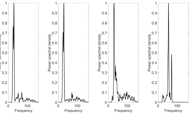
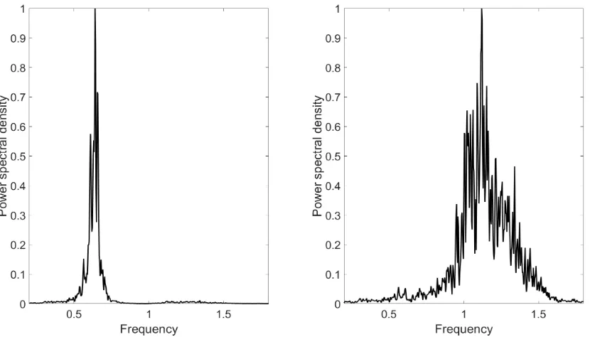
Fig.2 shows the results of PSDs for the simulated physical variables. Both

modes are present in the PSDs for the physical coordinates, which shows that

PSD of displacement and the frequency is in Hz.

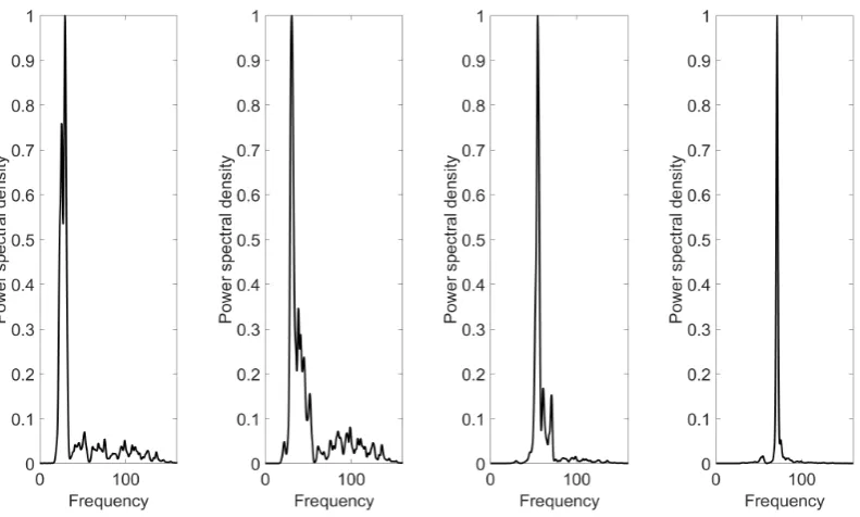
As can be seen in Fig.3, PCA fails in decoupling the nonlinear system (standard

linear modal analysis) but kernel ICA, as seen in Fig.4, has successfully

decoupled the nonlinear system into two SDOF systems due to the removal

of the higher order statistical dependence. Standard linear modal analysis

is equivalent to PCA in this case as the mass matrix is diagonal. PCA

as already mentioned can compute the new transformed variables (called

principal components) as linear combinations of the original variables. The

first principal component is required to have the largest possible variance. This

approach means that PCA can decompose only up to second-order/moment

statistics where all components that are computed, are under the constraint

of being orthogonal to the first component and to have the largest possible

inertia. And this is the basic reason that PCA is under-performing when

strong nonlinearities are present as the dependencies are moving away from

second-order statistics correlations.

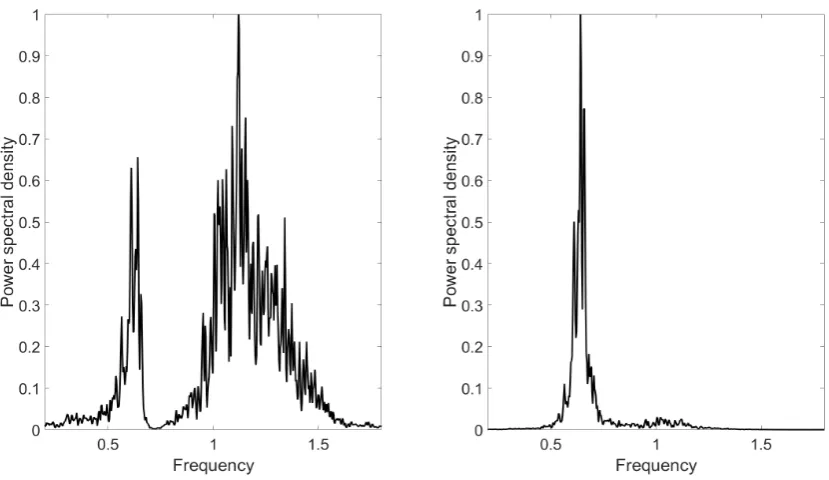
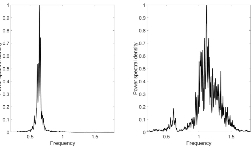
Furthermore, in Fig.5 LLE gives even better results for KICA, as the

decou-pling, is even more visual and effective and this is something that the reader

should keep in mind as it will be presented in the next sections.

To be very clear the results are presented in order of natural frequencies of

the examined system and the associated decoupled SDOF systems from the

Figure 1: Nonlinear two-DOF lumped parameter system.

Figure 3: PSDs for transformed variables: linear modal analysis (PCA).

Figure 5: PSDs for transformed variables: local linear embedding.

6. A three-degree-of-freedom system

In order to validate the results further, a more complicated system in terms

of degrees of freedom is discussed. The system of interest will be a nonlinear

three-DOF lumped parameter system. Data were simulated using a 4th_-order

Runge-Kutta algorithm and the excitation was chosen to be a Gaussian

displacements were extracted.     

m 0 0

0 m 0

0 0 m

              ¨ y1 ¨ y2 ¨ y3          +     

2c −c 0

−c 2c −c

0 −c 2c

              ˙ y1 ˙ y2 ˙ y3          +     

2k −k 0

−k 2k −k

0 −k 2k

              y1 y2 y3         

+k3

         y3 1 0 0          =          x1 0 0          (14)

The model parameters adopted were: m = 1, c = 0.1, k = 10, k3 = 1500.

Again, the damping is proportional, so the underlying linear system uncouples.

In total, 100,000 points were simulated; these were mainly used in order to

estimate the spectral densities as shown later and, only 2000 points were used

for the training of the machine learning algorithms.

As can be seen in Figs. 6-8, both PCA and kernel ICA lack efficiency and

performance in decoupling the nonlinear modes of the system. This is the

reason that a novel approach to structural dynamics is introduced next in

the form of the local linear embedding method. In Fig.9 the LLE method is

shown to successfully decouple the modes as it was able to unfold and learn

the underlying nonlinear manifold.

As can be seen in this section, the combination of stronger nonlinearity

with multi-degree of freedom systems makes the performance of both the

PCA and ICA algorithm very weak (see Fig. 6-8). Neither of them can

decouple successfully the nonlinear modes. This is the reason that

locally-linear- embedding is adapted as a quick, very simple and effective method of

Figure 6: PSDs for physical variables.

Figure 8: PSDs for transformed variables: Kernel ICA.

7. An experimental validation

The final case study is a further investigation of the methods based on an

experimental setup (see Fig.10). The full description of the experiment can be

viewed in [33, 34]. Briefly, the measurements were collected from a ‘bookshelf’

structure at the Engineering Institute from Los Alamos National Laboratories

[33, 34]. The model is a three-storey base-excited structure. Within the remits

of this linear structure, it is possible to introduce nonlinear dynamics via a

bumper mechanism between the top two floors, which introduces a nonlinear

contact mechanism. The broadband base excitation was between 20-150 Hz

and in relative co-ordinates this gives three ‘modes’, but the time series of

the four accelerations are used as all of them carry important information for

the transformations.

It is evident from Figs.11-14, that the conclusions derived from the previous

simulated models, are also valid in the experimental investigation. PCA fails

in decoupling the nonlinear system but kernel ICA and LLE compete in

effectiveness with the LLE being slightly more powerful overall due to its

Figure 10: Test structure architecture [33, 34].

Figure 12: PSDs for transformed variables: linear modal analysis (PCA).

Figure 14: PSDs for transformed variables: local linear embedding.

8. Conclusion & discussion

The purpose of this paper is to highlight the key utility of some advanced

and representative machine learning methods, not only for dynamic analysis

of structures but also as a method of dimension reduction for nonlinear

mechanical systems. The main benefit of the approach taken here is that

complicated algebraic analysis is not necessary. Furthermore, the physical

equations of the system are not needed.

At this point the authors need to include a comment about some previous

work in [12], as this paper is a continuation of [12], via another perspective and

path. In [12], one has to form a cost function and an optimisation problem.

This cost function (or objective function) has to be defined by the user by

which minimised all correlations up to third order is implemented in [12]

where to simplify the computation, the terms with velocities were disregarded.

Furthermore, a penalty function was used to impose orthogonality on the

polynomial coefficient vectors obtained after the optimisation. However, it

is cloudy what constraints should be used for the nonlinear problem as the

transformation is nonlinear. Also, as the authors use the same case studies

as in [12] one can see that the results are giving a slightly better resolution

and separation compared to the previous mentioned work (especially for the

three-DOF system and the experimental case study).

The biggest advantage of the approach presented here is that one needs

not necessarily worry about the majority of the analytical formulations.

Furthermore one can build for several datasets, the nonlinear subspace learning

only once and construct directly a forward and inverse transformation in an

unsupervised and nonparametric black-box path. Also, one can even use

supervised regression techniques like Gaussian processes as in [12] (which is a

very clever way to construct an inverse problem in a semi-supervised learning

manner).

A significant disadvantage regarding LLE for example (compared to ICA), is

that LLE, although it can easily be trained with small data sets and then

project new data as it comes it can not project low-dimensional data back

into the data space as back projection/reconstruction can be implemented

easily for linear techniques or ICA or AANN ([22, 23]) but not for sparse

spectral dimensionality reduction techniques like LLE or Laplacian eigenmaps.

PCA (or ICA in some extent), for example, can go forward or backward

into the space because it forms an eigendecomposition of a full matrix. But

LLE as described computes a graph representation of the data points and

local properties leads to an embedding of non-convex manifold by writing the

high-dimensional data as a combination of their nearest neighbours and as

a result in the low-dimensional representation of the data, LLE attempts to

retain the reconstruction weights making the direct and accurate projection

of low-dimensional data back into high-dimensional space very difficult or

impossible [22, 23]. But one can use a similar clever path as in [12] for an

inverse formulation.

Another big contribution of this work is that it opens the path for nonlinear

operational modal analysis through video or image data (as in [35, 36]) using

pure machine learning unsupervised techniques for blind source separation. As

a result, this machine learning approach is suited to experimental investigation

of nonlinear systems using only the measured output responses. Obviously,

the methods presented here are not a panacea and the purpose of this

study is to promote the usage of such tools that share a machine learning

nature for nonlinear dynamics in an potential practical application away from

conventional and classic methods.

Acknowledgments

The support of the UK Engineering and Physical Sciences Research Council

(EPSRC) through grant reference number EP/J016942/1 and EP/K003836/2

is gratefully acknowledged.

References

[1] G. Kerschen, J.-C. Golinval, A. F. Vakakis, L. A. Bergman, The method

order reduction of mechanical systems: an overview, Nonlinear dynamics

41 (1-3) (2005) 147–169.

[2] A. F. Vakakis, Non-linear normal modes (nnms) and their applications in

vibration theory: an overview, Mechanical systems and signal processing

11 (1) (1997) 3–22.

[3] G. R. Tomlinson, K. Worden, Nonlinearity in structural dynamics:

de-tection, identification and modelling, CRC Press, 2000.

[4] K. Worden, G. R. Tomlinson, Nonlinearity in experimental modal

analy-sis, Philosophical Transactions of the Royal Society of London A:

Math-ematical, Physical and Engineering Sciences 359 (1778) (2001) 113–130.

[5] K. Worden, P. L. Green, A machine learning approach to nonlinear

modal analysis, in: Dynamics of Civil Structures, Volume 4, Springer,

2014, pp. 521–528.

[6] R. M. Rosenberg, The normal modes of nonlinear n-degree-of-freedom

systems, Journal of applied Mechanics 29 (1) (1962) 7–14.

[7] S. W. Shaw, C. Pierre, Normal modes for non-linear vibratory systems,

Journal of sound and vibration 164 (1) (1993) 85–124.

[8] S. A. Neild, D. J. Wagg, Applying the method of normal forms to

second-order nonlinear vibration problems, in: Proceedings of the Royal Society

of London A: Mathematical, Physical and Engineering Sciences, Vol. 467,

The Royal Society, 2011, pp. 1141–1163.

[9] F. Poncelet, G. Kerschen, J.-C. Golinval, D. Verhelst, Output-only modal

analysis using blind source separation techniques, Mechanical systems

[10] J. Murdock, Normal forms and unfoldings for local dynamical systems,

Springer Science & Business Media, 2006.

[11] D. J. Ewins, Modal testing: theory and practice, Vol. 15, Research

studies press Letchworth, 1984.

[12] K. Worden, P. L. Green, A machine learning approach to nonlinear modal

analysis, Mechanical Systems and Signal Processing 84 (2017) 34–53.

[13] C. M. Bishop, Pattern Recognition and Machine Learning,

Springer-Verlag New York, 2016.

[14] C. M. Bishop, Neural networks for pattern recognition, Oxford university

press, 1995.

[15] I. Nabney, NETLAB: algorithms for pattern recognition, Springer Science

& Business Media, 2002.

[16] A. Hyv¨arinen, E. Oja, A fast fixed-point algorithm for independent

component analysis, Neural computation 9 (7) (1997) 1483–1492.

[17] H. G¨avert, J. Hurri, J. S¨arel¨a, A. Hyv¨arinen, The fastica package for

matlab, Lab. of Computer and Information Science, Helsinki University

of Technology.

[18] F. R. Bach, M. I. Jordan, Kernel independent component analysis, The

Journal of Machine Learning Research 3 (2003) 1–48.

[19] D. T. Pham, Contrast functions for blind separation and deconvolution

[20] L. K. Saul, S. T. Roweis, An introduction to locally linear embedding,

Available at: http://www. cs. toronto. edu/˜ roweis/lle/publications.

html.

[21] S. T. Roweis, L. K. Saul, Nonlinear dimensionality reduction by locally

linear embedding, science 290 (5500) (2000) 2323–2326.

[22] L. Van Der Maaten, E. Postma, J. Van den Herik, Dimensionality

reduction: a comparative, J Mach Learn Res 10 (2009) 66–71.

[23] L. v. d. Maaten, G. Hinton, Visualizing data using t-sne, Journal of

machine learning research 9 (Nov) (2008) 2579–2605.

[24] H. Bourlard, Y. Kamp, Auto-association by multilayer perceptrons and

singular value decomposition, Biological cybernetics 59 (4-5) (1988)

291–294.

[25] M. Scholz, R. Vig´ario, Nonlinear pca: a new hierarchical approach., in:

ESANN, 2002, pp. 439–444.

[26] N. Dervilis, M. Choi, S. Taylor, R. Barthorpe, G. Park, C. Farrar,

K. Worden, On damage diagnosis for a wind turbine blade using pattern

recognition, Journal of sound and vibration 333 (6) (2014) 1833–1850.

[27] N. Japkowicz, S. J. Hanson, M. A. Gluck, Nonlinear autoassociation is

not equivalent to pca, Neural computation 12 (3) (2000) 531–545.

[28] M. A. Kramer, Nonlinear principal component analysis using

autoasso-ciative neural networks, AIChE journal 37 (2) (1991) 233–243.

[29] K. Worden, Structural fault detection using a novelty measure, Journal

[30] L. Tarassenko, A. Nairac, N. Townsend, I. Buxton, P. Cowley, Novelty

detection for the identification of abnormalities, International Journal of

Systems Science 31 (11) (2000) 1427–1439.

[31] G. Kerschen, J.-C. Golinval, Feature extraction using auto-associative

neural networks, Smart Materials and Structures 13 (1) (2003) 211.

[32] P. Welch, The use of fast fourier transform for the estimation of power

spectra: a method based on time averaging over short, modified

peri-odograms, IEEE Transactions on audio and electroacoustics 15 (2) (1967)

70–73.

[33] E. Figueiredo, G. Park, J. Figueiras, C. Farrar, K. Worden, Structural

health monitoring algorithm comparisons using standard data sets, Tech.

rep., Los Alamos National Lab.(LANL), Los Alamos, NM (United States)

(2009).

[34] E. Figueiredo, E. Flynn, Three-story building structure to detect

nonlin-ear effects, Report SHMTools data description.

[35] Y. Yang, C. Dorn, T. Mancini, Z. Talken, G. Kenyon, C. Farrar, D.

Mas-care˜nas, Blind identification of full-field vibration modes from video

measurements with phase-based video motion magnification, Mechanical

Systems and Signal Processing 85 (2017) 567–590.

[36] S. Dasari, C. Dorn, Y. Yang, C. Farrar, A. Larson, D. Mascare˜nas,

Extraction of full-field structural dynamics from digital video

measure-ments in presence of large rigid body motion, in: Shock & Vibration,

Aircraft/Aerospace, Energy Harvesting, Acoustics & Optics, Volume 9,