City, University of London Institutional Repository
Citation
:
Ballotta, L. and Kyprianou, A.E. (2001). A note on the alpha-quantile option. Applied Mathematical Finance, 8(3), pp. 137-144. doi: 10.1080/13504860210122375This is the accepted version of the paper.
This version of the publication may differ from the final published
version.
Permanent repository link:
http://openaccess.city.ac.uk/5809/Link to published version
:
http://dx.doi.org/10.1080/13504860210122375Copyright and reuse:
City Research Online aims to make research
outputs of City, University of London available to a wider audience.
Copyright and Moral Rights remain with the author(s) and/or copyright
holders. URLs from City Research Online may be freely distributed and
linked to.
City Research Online: http://openaccess.city.ac.uk/ [email protected]
A note on the
α
-quantile option
Laura Ballotta
1and Andreas E. Kyprianou
2December 2001
1Department of Actuarial Science and Statistics, City University, London EC1V
0HB, UK.e-mail: [email protected]
2Mathematisch Instituut, Budapestlaan 6, 3584CD, Utrecht, The Netherlands.
Abstract
In this communication, we discuss some properties of a class of path depen-dent options based on the α-quantiles of Brownian motion. In particular we show that such options are well behaved in relation to standard options and comparatively cheaper than an equivalent class of lookback options.
1
Introduction
A new type of path-dependent option which can be interpreted as a mod-ification of lookback options is the α-quantile option, proposed recently by Miura (1992). Its payoff at maturity is defined by the order statistics of the underlying asset price; in particular, this order statistic or, better, the
α-percentile point of the stock price for 0< α < 1 can be thought of as the level at which the price stays below for 100α% of the time during the option’s contract period. The problem of pricing such an option has motivated stud-ies concerning the propertstud-ies of the distribution function of the α-percentile of the stochastic process driving the stock price, which has been investigated mainly by Akahori (1995), Dassios (1995, 1996), Tak´acs (1996), Yor (1996) and Doney and Yor (1998). Closed formulas in the traditional Black-Scholes framework for the price of this option have been obtained both by Dassios (1995) and Akahori (1995) who also provides an analytical expression for the hedging strategy. However, these formulas are still expressed in integral form, which could present serious computational difficulties if they are to be evaluated numerically.
The present paper proposes a numerical method to simulate theα-quantile option price. Such an approach takes advantage of the Dassios-Port-Wendel identity concerning the α-quantile of a Brownian motion with drift, rather than using numerical integration procedures. The results obtained from this method are then discussed.
2
Pricing
α
-quantile options
Let (Wt:t≥0) be a one-dimensional standard Brownian motion with W0 =
0; letσ∈R+,µ∈
Rand defineX = (Xt:t ≥0) as an arithmetic Brownian
motion such that
Xt=µt+σWt.
The α-quantile of X over the interval [0, t] is defined as follows.
Definition 1 Let Γ (a, t) =Rt
0 1(Xs≤a)ds be the occupation time of a
Brown-ian motion with drift, Xt. The α-quantile of Xt is defined as
Q(α, t) = inf{x: Γ (x, t)> αt}
From this definition it follows that Q(α, T) ≤ sup0≤t≤T Xt a.s. and
Q(α, T)≥inf0≤t≤T Xt a.s. More precisely
lim
α→0Q(α, T) = 0≤inft≤TXt a.s.
lim
α→1Q(α, T) = 0sup≤t≤T
Xt a.s.
An important result related to the α-quantile concerns its distribution function. Dassios (1995) obtained a useful representation of such a function analogous to a decomposition for random walks due to Wendel (1960) and Port (1963).
Theorem 2 (Dassios-Port-Wendel identity) Let 0< α <1, then
Q(α, T)= supd
0≤t≤αT
Xt+ inf
0≤t≤(1−α)T
˜
Xt, (1)
where =d means equality in distribution and X˜t is an independent copy of the
arithmetic Brownian motion.
Consider now the Black-Scholes framework. The non-dividend paying risky asset S has value St = S0eXt at time t ≥ 0 where S0 > 0. Further,
the return on the riskless bond is exponential with rate r > 0. Then an α -quantile call option with strike price K and underlying asset S has a payoff function at maturity date, T, defined as S0eQ(α,T)−K
+
, where S0 is the
value of the underlying asset at the beginning of the contract and Q(α, T) is the α-quantile of X. Analogously, the payoff of an α-quantile put option of the same type is K−S0eQ(α,T)
+
.
Applying the risk-neutral valuation procedure (Harrison and Pliska, 1981), we can say that the no-arbitrage price at time t∈[0, T] of an α-quantile call option is given by
C(S0, α, T −t) = e−r(T−t)E
h
S0eQ(α,T)−K
+
| Ft
i
,
where {Ft}t≥0 is the natural filtration for X and E denotes the expectation
under the risk-neutral probability measureP. The price of theα-quantile put can be defined analogously. Exploiting the convolution property in Theorem 1, Dassios (1995) also obtained the closed formula for the α-quantile call option
C(S0, α, T −t) = e−r(T−t)
Z ∞
K P
˜
Q(α′
, T −t)>ln z
St | Ft
1
Γln z S0,t
>t−(1−α)Tdz
+e−r(T−t)
Z ∞
K
1
Γln z S0,t
≤t−(1−α)Tdz, (2)
where
α′
= αT −Γ
lnSz0, t T −t
and ˜Q(., .) is a version of the α-quantile that is independent ofFt.
Given the nature of the α-quantile of a Brownian motion, the α-quantile option can be considered as a “smoothed” version of a more well-known path-dependent option, the fixed strike lookback option. It can be shown quite easily that the α-quantile option is always cheaper than an equivalent lookback option written on the same underlying, with the same strike K, same expiration dateT and lookback period [0, T]. Specifically, consider the case of a call option. The payoff at maturity of the fixed strike lookback call is S0eM
T
0 −K
+
, where MT
0 = sup0≤t≤T Xt. Its price at time t is then
L(S0, T −t) =e−r(T−t)E
S0eM
T
0 −K
+
| Ft
.
Since Q(α, T)≤MT
0 a.s., it follows that
Y := S0eQ(α,T)−K
+
−S0eM
T
0 −K
+
≤0 a.s. (3)
Setting Z = E[Y | Ft], inequality (3) and the definition of conditional
ex-pectation imply
E[Z1A] =E[Y1A]≤0 ∀A∈ Ft.
Hence it follows that
C(S0, α, T −t)≤L(S0, T −t) a.s. (4)
By an analogous argument it is possible to show that also the put option is always less expensive than the fixed strike lookback put. This analytical result is confirmed by the numerical evidence produced in the next section.
3
Monte Carlo simulation
As observed in the previous section, analytic pricing formulas for the α -quantile option are difficult to compute. As we can see from equation (2), in fact, the closed valuation formula of this option requires that all the occupa-tion times nΓln z
S0, t
the α-quantile, which can be obtained through the convolution property of Theorem 1. That means computing another integral expression. On the other hand Theorem 1 and the fact that the distributions of the extremes of the Brownian motion are well known results (see for example Karatzas and Shreve, 1997), provide a straightforward framework to produce the price of the α-quantile option. The idea is to use a Monte Carlo valuation procedure for the price at time 0 of the quantile option, in which the α-quantile of the Brownian motion is generated directly as the sum of two independent sam-ples of the extremes of X. More precisely, the approach can be described by the following steps:
• for i = 1,2, ..., n generate independent samples of M := sup
0≤t≤αT
Xt and
m := inf
0≤t≤(1−α)TXt by inversion of their distribution functions, through
the Newton algorithm;
• let Qi be the sum of the independent realizations of M and m, then
the final payoff, Yi, of the α-quantile option is computed as Yi =
S0eQi −K
+
;
• let ˆC :=e−rT Pn
i=1Yi/n; then ˆC is a numerical approximation to the
option price at time t = 0.
Note that in this way we don’t need to generate the entire history of the Brownian motion; a procedure that presents problems when choosing an appropriate approximating random walk. Since the α-quantile option is a path-dependent contract, its value is liable to be sensitive to the frequency with which the extremes of the Brownian motion are observed. For a random walk approximation, the “true” extremes of the Brownian motion may not be correctly sampled.
In the same framework, this Monte Carlo procedure can be adapted to approximate also the delta of the α-quantile option at time 0. Let ∂i :=
eQi1
(S0eQi>K) be the partial derivative of the sample payoff Yi with respect
to S0. Then ∆ = e−rTPni=1∂i/n is a numerical approximation to the α
-quantile option delta at time t = 0. To be precise a closed form for the option delta has been derived, as already mentioned, by Akahori (1995). However such a formula suffers of the same problem of the option price, that is it is still expressed in integral form involving also the distribution function of the α-quantile.
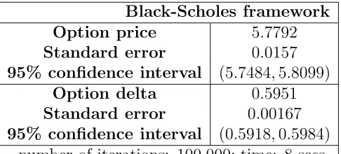
The Monte Carlo simulation has been carried out by generating 100,000 paths. Using a C++ program on a desktop with Pentium(r) III processor
and 64,0 MB RAM, the numerical procedure implemented takes 8 seconds to return the option price. The control variate technique is used to reduce the variance of the obtained estimates. The benchmark contract is chosen to be the lookback counterpart; hence the option contract is computed as
ˆ
CCV
q = ˆCq+β
CL−CˆL
,
where ˆCq is the price of the quantile call option obtained by the procedure
described above, CL is the exact price of a lookback call contract written
on the same underlying, with equal maturity and strike and lookback pe-riod [0, T], ˆCL is the estimated value for such a lookback option using a
Monte Carlo procedure, and β is a parameter with value other than one. In particular, the choice of β which minimizes the option price variance is
β∗ =CovCˆ
q,CˆL
/V arCˆL
. In order to avoid the introduction of a bias in the estimation of the option price, we use a few pilot runs to estimate β∗ and then we use this parameter in the main simulation run. The details of the output for the quantile option are presented in Table 1. We choose this version of the control variate technique because β∗ allows to reduce signifi-cantly the option variance no matter the level ofα chosen, that is no matter the degree of correlation between the quantile option and the lookback. In fact, we have to consider that the quantile option loses any similarity with the lookback counterpart for values of α far enough from 1.
4
Simulated prices
Throughout all the following analysis, unless otherwise stated, the basic pa-rameter set is
S0 = 100; K = 100; α = 0.5; r = 0.05; σ = 0.2; T = 1.
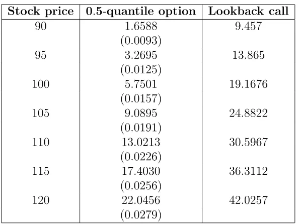
Theα-quantile call price for different values of the initial stock price, with all the other parameters left unchanged, is given in Table 2. In the same table we report also the price of a fixed strike lookback call1 written on the same
underlying and computed for the same values of the parameters K, r, σ and
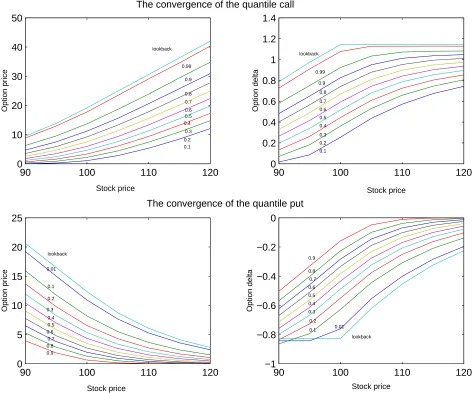
T. As expected, the 0.5-quantile option is cheaper than the lookback option. In order to observe empirically the convergence property of the α-quantile option to the lookback option discussed in the previous section (see equation (4)), for the particular case of t = 0, in Figure 1 we plot the prices of both
1The price in this case in computed through its closed formula (Conze and Viswanathan,
the α-quantile call and put against the stock price for different values of the parameter α. Also, we add to the plot the price function of the equivalent lookback. The dominating value of the lookback as discussed in section 2 is clear. The same kind of analysis is extended to the delta of the options considered and the results are given in Figure 1.b and 1.d. In general, we can say that the slope of the delta when it is considered a function of the stock price represents the option’s gamma. Gamma provides informations about the frequency with which a possible portfolio containing such an option has to be rebalanced in order to maintain a perfect hedge. Hence, it is reasonable to expect that, when the stock price is in the neighborhood of the strike price, the delta is highly sensitive to changes in the underlying asset price, therefore the portfolio is likely to be rebalanced very frequently. Let us now consider the case of the call option. As the stock price becomes very large, delta becomes less sensitive because the option is expected to expire in-the-money. This is the behaviour we can observe in Figure 1.b. For the case of the lookback option this behaviour is very marked. If the initial value of the stock is equal to the strike price, the maximum of the stock itself cannot be less than the strike price. Therefore, above this “critical value” there is no additional risk to hedge and the delta remains constant. The pattern for the α-quantile option, instead, is more “smoothed”, but asα approaches the unity we see that the pattern of the delta becomes more and more similar to the one of the lookback, due again to the convergence property of the α -quantile option to the lookback option. Analogous considerations hold also for the put case with the (obvious) difference that the delta becomes less sensitive when the stock price becomes smaller with respect to the strike price.
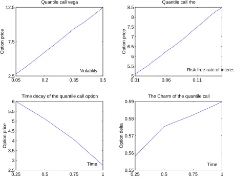
A general study of comparative statics concerning all the main parame-ters on which the option value depends, reveals that the α-quantile option presents patterns lined up with the behaviour of other Euro-type options. For example, in Figure 2 it is shown the sensitivity of the α-quantile call option to changes in the stock volatility. As we can observe, the option price is positively correlated with σ, which is again a common feature of all op-tions. In fact, the volatility represents a measure of the uncertainty of the stock price future movements. Since a call option has limited downside risk in the event of stock price falls, the value the option tends to increase when the volatility increases as well. Figure 2 contains also other option greeks, like the rho, which represents the sensitivity of the contract price to changes in the interest rate, as well as the time decay of the contract, the so-called theta, and the charm, that is the rate at which the delta changes with time to maturity. Analogous results can be also obtained for the put option.
5
Conclusions
In this note we have presented properties and features of a new financial instrument, the α-quantile option, introduced first by Miura (1992), which is at the moment only a “theoretical” object since it is not yet traded in the market. The Dassios-Port-Wendel identity has been employed to simulate initial prices and Greeks of theα-quantile. In view of the analytical structure of this option the simulations not surprisingly show consistent characteristics to other Euro-type option contracts. The problem of obtaining numerically the mid-contract value of the option remains unsolved. In fact, for this case pricing formulas and numerical approximations cannot avoid the set of occupation times needed to define the α-quantile itself and which makes this process not Markovian.
6
Acknowledgments
The first author worked under the financial support of a Ph.D. scholarship from the University of Bergamo for which she expresses great thanks. Fur-thermore, thanks are due to Prof. Christian Schlag for his helpful comments about some aspects of the work.
References
[1] Akahori J. (1995): Some formulae for a new type of path-dependent option, The Annals of Applied Probability, 5, 383-388.
[2] Conze, A. and Viswanathan (1991): Path dependent options: the case of lookback options, The Journal of Finance, 46, 1893-1907.
[3] Dassios A. (1995): The distribution of the quantile of a Brownian motion with drift and the pricing of related path-dependent options,The Annals of Applied Probability, 5, 389-398.
[4] Dassios A. (1996): Sample quantiles of stochastic processes with sta-tionary and independent increments, The Annals of Applied Probability, 6, 1041-1043.
[6] Harrison M. and S. R. Pliska (1981): Martingales and Stochastic In-tegrals in the Theory of Continuous Trading, Stochastic Processes and their Applications, 215-260.
[7] Karatzas I., Shreve S. E., Brownian Motion and Stochastic Calculus, Springer, 1997.
[8] Miura R. (1992): A note on lookback options based on order statistics, Hitotsubashi Journal of Commerce and Management, 27, 15-28.
[9] Port S. C. (1963): An Elementary Probability Approach to Fluctuation Theory, Journal of Mathematical Analysis and Applications, 6, 109-151.
[10] Tak´acs L. (1996): On a generalization of the arc-sine law, The Annals of Applied Probability, 6, 1035-1040.
[11] Wendel J. G. (1960): Order Statistics of Partial Sums, Annals of Math-ematical Statistics, Vol. 31, 1034-1044.
[12] Yor M. (1995): The distribution of Brownian quantiles, Journal of Ap-plied Probability, 32, 405-416.
90 100 110 120 0 10 20 30 40 50 0.2 0.3 0.1 0.99 lookback 0.8 0.7 0.9 0.5 0.4 0.6 Stock price Option price
90 100 110 120
0 0.2 0.4 0.6 0.8 1 1.2 1.4 Option delta
90 100 110 120
0 5 10 15 20 25 Option price
90 100 110 120
−1 −0.8 −0.6 −0.4 −0.2 0 Option delta
The convergence of the quantile call
The convergence of the quantile put
Stock price
Stock price Stock price
[image:12.612.104.580.85.478.2]lookback lookback lookback 0.99 0.01 0.01 0.9 0.9 0.9 0.8 0.8 0.8 0.7 0.7 0.7 0.6 0.6 0.6 0.5 0.5 0.5 0.4 0.4 0.4 0.3 0.3 0.3 0.2 0.2 0.2 0.1 0.1 0.1
0.05 0.2 0.35 0.5 2.5
7.5 12.5
Volatility
Option price
Quantile call vega
0.015 0.06 0.11 5.5
6 6.5 7 7.5 8 8.5
Risk free rate of interest
Option price
Quantile call rho
0.25 0.5 0.75 1 2.5
3 3.5 4 4.5 5 5.5 6
Time
Option price
Time decay of the quantile call option
0.25 0.5 0.75 1 0.55
0.56 0.57 0.58 0.59
Time
Option delta
[image:13.612.105.562.84.433.2]The Charm of the quantile call
Figure 2: The sensitivity of the α-quantile call option to changes in the stock
volatility, the rate of interest and the time to maturity.
Black-Scholes framework Option price 5.7792 Standard error 0.0157 95% confidence interval (5.7484,5.8099)
Option delta 0.5951 Standard error 0.00167 95% confidence interval (0.5918,0.5984)
[image:14.612.177.420.296.406.2]number of iterations: 100,000; time: 8 secs.
Stock price 0.5-quantile option Lookback call
90 1.6588 9.457
(0.0093)
95 3.2695 13.865
(0.0125)
100 5.7501 19.1676
(0.0157)
105 9.0895 24.8822
(0.0191)
110 13.0213 30.5967
(0.0226)
115 17.4030 36.3112
(0.0256)
120 22.0456 42.0257
[image:15.612.150.446.243.466.2](0.0279)
Table 2: The α-quantile call price and the lookback call. The numbers in
paren-theses correspond to the standard errors of the Monte Carlo simulations.