Random Rectangular Graphs
Ernesto Estrada and Matthew Sheerin
A generalization of the random geometric graph (RGG) model is proposed by considering a set of points uniformly and independently distributed on a rectangle of unit area instead of on a unit square [0,1]2. The topological properties, such as connectivity, average degree, average path length and clustering, of the random rectangular graphs (RRGs) generated by this model are then studied as a function of the rectangle sides lengths a and b= 1/a, and the radius rused to connect the nodes. Whena= 1 we recover the RGG, and whena → ∞ the very elongated rectangle generated resembles a one-dimensional RGG. We provided computational and analytical evidence that the topological properties of the RRG dier signicantly from those of the RGG. The connectivity of the RRG depends not only on the number of nodes as in the case of the RGG, but also on the side length of the rectangle. As the rectangle is more elongated the critical radius for connectivity increases following rst a power-law and then a linear trend. Also, as the rectangle becomes more elongated the average distance between the nodes of the graphs increases, but the local cliquishness of the graphs also increases thus producing graphs which are relatively long and highly locally connected. Finally, we found the analytic expression for the average degree in the RRG as a function of the rectangle side lengths and the radius. For dierent values of the side length, the expected and the observed values of the average degree display excellent correlation, with correlation coecients larger than 0.9999.
PACS: 89.75.-k; 02.10.Ox
I. INTRODUCTION
model that allows us to evaluate which properties of the system have arisen from their connectivity pattern. In this sense, the common election is the use of random graphs. That are graphs with the same number of nodes and edges as the one under study, but in which the connection between the nodes is made randomly and independently [6]. There are several of these random models of great usability in current network theory, such as the Erdös-Rényi [8], the Barabási-Albert [9] or the Watts-Strogatz [10] model to mention just three.
In many real-world scenarios the networks emerge under certain geometrical constraints. This is the case of the so-called spatial networks [11], which include infrastructural networks such as road networks, airport transportation networks, etc., [11] and certain biological networks such as brain networks or the networks representing the proximity of cells in a biological tissue (see [3]). The list also includes the networks of patches and corridors in a landscape [12], the networks of galleries in animal nests [13, 14], and the networks of fractures in rocks [15], among others. The classical election of a random graph used to represent these systems are the so-called random geometric graphs [16, 17]. Here the term random geometric graph (RGG) is reserved for the case in which the nodes of the graph are distributed randomly and independently in a unit square and two nodes are connected if they are inside a disk of a given radius. Other graphs in which the edges are constructed by using dierent geometric rules will be named here generically as random proximity graphs.
RGGs have found important applications in the area of wireless communication devices [1820], such as mobile phones, wireless computing systems, wireless sensor networks, etc. This was indeed the rst application in mind when Gilbert proposed the very rst RGG model [21]. RGGs have also found applications in areas such as modelling of epidemic spreading in spatial populations, which may include cases such the spreading of worms in a computer network, viruses in a human population, or rumors in a social network [22 26]. RGGs have been used to describe how cities have been evolving under the geometric constraints imposed by their geographic locations [27]. For a wider perspective on the applications of spatial graphs the reader is referred to the review [11].
Here, we develop a new model that generalizes the RGG by allowing the embedding of the nodes in a unit rectangle instead of a unit square. Our main goal is to investigate how the elongation of a unit square inuences the topological properties of the graphs generated by the model. This generalized graphs will be named here the random rectangular graphs (RRGs). In this work we concentrate on the inuence of the ratio of the lengths of the two sides of the rectangle on the topological properties of the graphs emerging on them, such as their connectivity, average degree, average path length and clustering coecient. In particular, we nd the analytical expression of the average degree. The average degree is a simple but highly important property of graphs, which is related to several dynamical processes.
II. DEFINITION OF THE MODEL
The RGG is dened in general by distributing uniformly and independently n points in the unit d-dimensional cube [0,1]d [16]. Then, two points are connected by an edge if their Euclidean distance is at most r, which is a given xed number known as the radius.
Let us now dene a unit hyperrectangle as the Cartesian product [a1, b1]×[a2, b2]× · · · ×
[ad, bd] where ai, bi ∈ R, ai ≤ bi, and 1 ≤ i ≤ d. Hereafter we will restrict ourselves to the
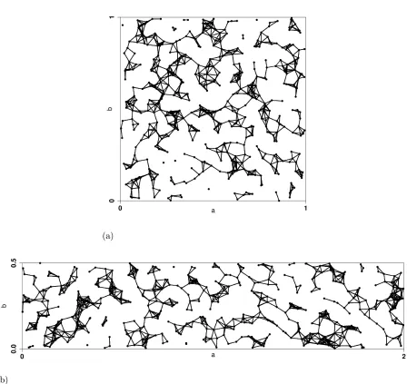
2-dimensional case, which corresponds to a rectangle of unit area, that we will call the unit rectangle. Now, the RRG is dened by distributing uniformly and independentlynpoints in the unit rectangle[a, b]and then connecting two points by an edge if their Euclidean distance is at most r. It is evident that the only change we have introduced here is to consider a rectangle of unit area instead of the analogous square. The rest of the construction process remains the same as for the RGG. This means that RRG → RGG as (a/b) → 1. In this sense we can say that the RRG is a generalization of the RGG. In Fig. 1 we illustrate an RGG and an RRG constructed with the same number of nodes and edges.
(a)
[image:5.612.76.524.64.487.2](b)
Figure 1. Illustration of two random rectangular graphs with a = 1 (top), which corresponds to
a random geometric graph on a unit square and with a= 2 (b= 0.5) (bottom). Both graphs are
built with 500 nodes and 1750 edges.
III. COMPUTATIONAL ANALYSIS OF RRG
In this section we study computationally a few topological properties of the RRGs. In the following we will consider RRGs with a= 1/b and consequently we will report only the value of a. For instance, a = 1 represents a unit square and the RRG is identical to the classical RGG. For a = 5 we have a very elongated rectangle with sides a = 5 and b = 0.2. We study here some important structural parameters of networks, such as the connectivity, average degree, average path length and the average clustering coecient.
3.1 Connectivity and average node degrees
In the case of the RGGs it is a well known result that increasing the radius of the disks centered at each point produces a phase transition from a disconnected to a connected graph at certain critical radius. That is, for
πr2 = logn+γn
n , (1)
the RGG is connected if n → ∞ and γn → ∞ and disconnected if γn → −∞ [16]. In
the Fig. 2(a) we illustrate this result for a RGG with n = 100 nodes, i.e., a = 1, where it can be seen that the critical radius is about 0.25, which corresponds to a value of γn ≈15.
As the square is elongated the critical radius increases with the value of a. For instance, for a= 5 the critical radius is about 0.5, and for a= 30 it is about 3. The main reason for this increase in the critical radius is that as we elongate the rectangle the points have to cover a longer region of the rectangle and as so their separation increases. As a consequence, we need to increase the radius in order to guarantee the connectivity of the network. As can be seen in the Fig. 2 (b) there is a linear trend between the length of the side of the rectangle and the critical radius of the RRGs for values ofa?5. For the values1≤a.5the relation between the critical radius and the side length of the rectangle is a power-law of the form rc∼a3.72.
(a)
0.0 0.5 1.0 1.5 2.0 2.5 3.0
0.0 0.2 0.4 0.6 0.8 1.0 r
Probability of being connected
0.0 0.5 1.0 1.5 2.0 2.5 3.0
0.0 0.2 0.4 0.6 0.8 1.0
0.0 0.5 1.0 1.5 2.0 2.5 3.0
0.0 0.2 0.4 0.6 0.8 1.0
0.0 0.5 1.0 1.5 2.0 2.5 3.0
0.0 0.2 0.4 0.6 0.8 1.0 a=1 a=5 a=10 a=30 (b)
0 5 10 15 20 25 30
0.5 1.0 1.5 2.0 2.5 a Cr itical r adius (c)
1 2 3 4 5
0.25 0.30 0.35 0.40 0.45 0.50 a Cr itical r adius
Figure 2. (color online) Probability that the RRG is connected as a function of the radius for
graphs withn= 100(a). Dependence of the critical radius for connectivity with the side length of
the rectangle for general (b) and small values of a(c). Every point is the average of 1000 random
realizations
[image:7.612.91.509.88.240.2]of the radius.
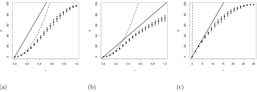
[image:8.612.93.509.119.268.2](a) (b) (c)
Figure 3. Illustration of the change in the average degree with the radius for (a) a random geometric graph in a unit square, (b) a random rectangular graph witha= 3, and (c) witha= 30. All graphs
haven= 100. The dotted line corresponds to the quadratic approximation ofhkiwithr (see text)
and the solid line corresponds to its linear approximation.
An important observation extracted from the plots of the average degree versus the radius is the existence of three dierent regimes in these plots. Due to their sigmoid shapes we observe that the dependance of the average degree with the radius is dierent for the regions 0 ≤ r ≤ b, b ≤ r ≤ a and a ≤ r ≤ √a2+b2. This is important because we will use these
three regimes for the analytic calculation of the average degree in general RRGs.
3.3 Average path length and clustering
Let Γ = (V, E) be a simple connected graph. A path of length k in Γ is a set of nodes i1, i2, . . . , ik, ik+1 such that for all 1 ≤ l ≤ k, (il, il+1) ∈ E with no repeated nodes. The
shortest-path or geodesic distance between two nodesu, v ∈V is dened as the length of the shortest path connecting these nodes. We will write d(u, v) to denote the distance between uandv. Here we will call, as usually in network theory, average path length to the following quantity:
hli= 2 n(n−1)
X
u<v
On the other hand, the local clustering coecient of a nodeu, which quanties the degree of transitivity of local relations in a network is dened as [10]:
Cu =
2|{(v, w) :v, w∈Nu; (v, w)∈E}|
ku(ku−1)
, (3)
where Nu = {v : (u, v) ∈ E} and ku is the degree of the node u. Taking the mean of
these values asu varies among the nodes inΓ, one gets the average clustering coecient of the network: hCi= 1
n
Pn
u=1Cu.
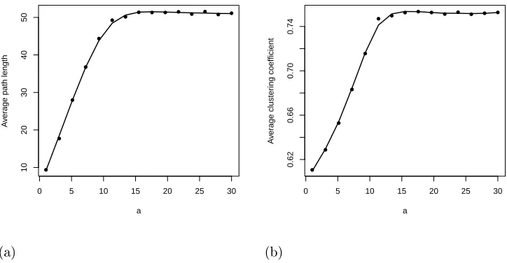
We study here graphs with 1000 nodes and 7500 edges. For every value of a we report the average of 10 random realizations. In the Fig. 4 we illustrate the variation of the average path length and average clustering coecients for these graphs. The plot of hli versus a agrees with our intuition that as we elongate the rectangle there are nodes which are more far apart from each other and as a result the average path length of the whole graph increases. There is an almost linear increase ofhlifor values of1≤a.15after which the dependence is very at. In this region we have that a → ∞, which corresponds to a good approximation to a one-dimensional RGG. Fora= 1 it is known that the average path length depends on the inverse of the radius, hlei=Θ(1/r) [31]. The actual radius used for
the plot in Fig. 4 isr = 0.0713 which gives an estimate of the average path length of 14.02, which is not too far from the observed value in the plot for a= 1. In the case of a= 30 we are in the presence of a very elongated rectangle, which is very similar to a one-dimensional RGG. A crude estimate of the average path length in this case would behlei=n/hki, which
in the current case will give hlei ≈ 66.6, which is relatively close to the observed value of
hli ≈50 for a= 30.
It is interesting to note that the average clustering coecient also increases as the rectan-gle becomes more elongated. This is a consequence of the fact that we are now compressing the nodes into a narrower region, which allow them to be locally closer to each other and create more triangles. However, as soon asa ≥15for these graphs (this value will depend on the number of nodes of the graph) the dependence of the average path length and clustering coecient with the side length is very at. This is due to the fact that for large enough values of a the graphs behave as a one-dimensional random geometric graph.
Let r2 = logn+γn
hCdi=
1−Hd(1) d even
3
2Hd(1/2) d odd,
(4)
where d is the dimension of the hypercube in which the nodes are embedded and
Hd(x) =
1 √
π
d/2
X
i=x
Γ (i) Γ i+12
3 4
i+12
, (5)
where Γ (i)is the Gamma function. Thus, for d = 2 , hC2i = 1−
3√3
4π ≈ 0.5865 and for d= 1,hC1i= 3/4 = 0.75.
As can be seen in the Fig. 4 for a = 1 the average clustering coecient is hCi ≈ 0.61, which is very close to the expected value for the 2-dimensional RGG. When a = 30 the average clustering coecient is hCi ≈ 0.75, which coincides with the exact value expected for the one-dimensional RGG. Consequently, the RRG generalizes the values of the clustering coecient of both, the one- and two-dimensional RGG, for a = 1 and a → ∞, respectively. In addition, it provides a series of intermediate values of the clustering coecient for intermediate values of the side length of the rectangle.
(a)
0 5 10 15 20 25 30
10
20
30
40
50
a
A
v
er
age path length
(b)
0 5 10 15 20 25 30
0.62
0.66
0.70
0.74
a
A
v
er
age cluster
[image:10.612.118.480.456.644.2]ing coefficient
Figure 4. Change of the average path length (left) and average clustering coecient (right) in a
RRG with the systematic variation of the side lengthaof the rectangle for graphs havingn= 1000
and hki = 15. Every point represents the average of 10 realizations. The standard deviations of
We now further explore the relation between the radius r and the average path length and clustering for RRGs with dierent side lengths. We consider graphs withn = 100nodes and the extreme cases a = 1 (RGG) and a = 30. As the radius increases the graph is becoming more and more dense, which is reected in the exponential decay of the average path length to the value hli = 1, which corresponds to that of a complete graph. There is not substantial dierences in the decay of the average path length with the increase of the radius for a= 1 and a= 30. For the average clustering coecient the results for both cases are very similar and they are characterized by an abrupt increase in the clustering at the beginning of the plot and then a linear increase until the value ofhCi= 1 is reached for the complete graph.
(a)
0 2 4 6 8 10
0 1 2 3 4 5 6 7 r A v er
age path length
0 2 4 6 8 10
0 1 2 3 4 5 6 7
0 2 4 6 8 10
0 1 2 3 4 5 6 7
0 2 4 6 8 10
0 1 2 3 4 5 6 7 a=1 a=5 a=10 a=30 (b)
0 1 2 3 4 5
0.0 0.2 0.4 0.6 0.8 1.0 r A v er age cluster ing coefficient
0 1 2 3 4 5
0.0 0.2 0.4 0.6 0.8 1.0
0 1 2 3 4 5
0.0 0.2 0.4 0.6 0.8 1.0
0 1 2 3 4 5
0.0 0.2 0.4 0.6 0.8 1.0 a=1 a=5 a=10 a=30
Figure 5. (color online) Variation of the average path length with the radius (a), as well as the variation of the average clustering coecient with the radius (b) for graphs with a = 1,5,10,30.
Every point is the average of 100 random realizations.
4 ANALYTICAL RESULTS FOR hki
Given a node, there aren−1nodes distributed in the rest of the rectangle. DeneAp to be the
area within radius r of a point pwhich lies within the rectangle. Since nodes are uniformly and independently distributed, the expected degree of a node vi is E(ki) = (n−1)Ai/(ab),
[image:11.612.118.481.312.504.2]between the area within distance r and the rest of the rectangle gives rise to the Binomial distributionBin(n−1, Ai/(ab))as it can be considered like a partition of a Poisson process.
Averaging this over all possible node locations (i.e., the points in the rectangle) gives
Ehki=
´
p{(n−1)Ap/(ab)}
ab =
(n−1)´pAp
(ab)2 (6)
Letf(a, b, r)to be the area within radiusrof a point which lies in the rectangle, integrated over all points, i.e., f(a, b, r) = ´pAp. Based on the computational results obtained for the
average degree we consider here the previously detected regions: 0≤ r ≤b, b ≤r ≤ a and a ≤ r ≤ √a2 +b2, recalling that a ≥ b. We call these cases i = 1,2,3, respectively. Thus,
the function f(a, b, r)takes dierent forms fi for each case i. This means that we can write
Ehki= (n−1)fi (ab)2 with
fi =
f1 0≤r ≤b
f2 b≤r≤a
f3 a≤r≤
√
a2+b2
(7)
and our task is now to nd the analytical expressions forfifor these three cases separately.
Case 1
This case corresponds to the covering of each point in the rectangle by a circle of small radius, 0≤r ≤b. Let us x a value of the radius to r. The area of this circle is A
, =πr
2.
Thus, if we consider intersecting circles covering the whole rectangle of area Ae = ab, the
total area covered is:
A
=A,A
e=πr2ab.
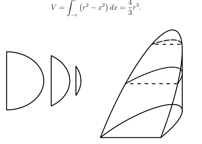
in such a way that they dene a section of a cylinder that has been intersected by a plane as illustrated in the Fig. 6. The sum of the areas of all these segments of the circle equals the contribution of one circle to the area outside the rectangle. This total area is easy to calculate by simply considering it equal to the volume of the section of the cylinder:
V =
ˆ r
−r
r2−x2
dx= 4 3r
[image:13.612.151.475.171.402.2]3. (8)
Figure 6. Illustration of the stacking of the segments of the circle which lie out the rectangle (left), and the section of the cylinder formed by all the stacked segments (right).
Using this volume, which corresponds to the area of a circle outside the rectangle, we can calculate the total area coming from all circles moving in the direction right-left (R-L) as well as those moving in the direction top-bottom (T-B). That is, the rst area is given by V b and the second is given by V a. The problem is that we are counting twice the area for some points which are in the square with arear2 which is located at each of the four corners
of the rectangle (see Fig. 7). In order to account for this area we consider a quarter of a circle (a pie) moving in the R-L direction and don't count the contribution for the area of the square at the corner. That is, we obtain the total areas in the R-L and T-B directions as:
AR−L=
1
2V(b−r), (9)
AT−B =
1
a
b
T−B
R−L
Figure 7. (color online) Illustration of a circle centered at a point inside the rectangle with sides a
and band separated from the edges of the rectangle by a distance equal to the radius of the circle
r. The arrows R-L and T-B indicate the directions of displacement of the circle used to calculate
the areas outside the rectangle. The square at the corner which has sides of length equal to r is
shadowed. the section of the circle which is inside this square corresponds exactly to a quarter of the circle.
For the area of the square at the corner we have already its contribution in the T-B direction. Now for contribution in the R-L direction we must consider that some quarter circles protrude both below and to the left of the rectangle. We then calculate the R-L contribution in such a way that we do not double-count anything
A
=
ˆ r
0
ˆ t
0
1 2 r
2−x2
dxdt= 5 24r
4. (11)
We are now in condition to calculate the total area of the circles covering only the space inside the rectangle when 0≤r≤b, which is
f1 =A−4 (AR−L+AT−B+A) (12)
=πr2ab− 4
3(a+b)r
3+1
2r
[image:14.612.210.416.115.251.2]Notice that we have multiplied the parenthesis in (12) by 4 because we have previously considered the areas of quarter circles.
Case 2
In this case every point is covered by a circle of radius, b ≤ r ≤ a. We take a similar approach to the one used in Case 1 with the following adaptation. Taking the bottom-left quadrant of the circle as before, there is always part of the quarter circle protruding from the bottom of the rectangle. Equivalently, every circle now protrudes from both the top and bottom of the rectangle. This makes certain geometric arguments used in Case 1 invalid, such that the one of being able to t a square of length r into the rectangle. For points at distance t from the top edge of the rectangle, the area of this protrusion is ´tr√r2−x2dx,
and integrating over t gives
V0 =
ˆ b
0
ˆ r
t
√
r2−x2dx dt
= 1 4πr
2
b−(1 3r
2
+ 1 6b
2
)√r2−b2−1
2r
2
barcsin(b r) +1
3r
3 (14)
This considers all the points in a vertical line through the rectangle, so we multiply by the length a to get
AT−B,2 =aV0 (15)
In this case we can no longer t a square of length r inside the rectangle, so we modify A
accordingly and obtain
A
,2 =
ˆ b 0 ˆ t 0 1 2 r
2−x2
dxdt
= 1 4r
2b2− 1
24b
4 (16)
We now obtain the total area f2 in a similar way as forf1
f2 =A−4(AT−B,2+A,2)
=−4 3ar
3−r2b2+ 1
6b
4+a(4
3r
2+ 2
3b
2)√r2−b2 + 2r2abarcsin(b
Case 3
In this case the circles have radiusa ≤r≤√a2+b2. Here we consider a slightly dierent
approach because the geometry of the system involved changes in relation to the previous cases. In this case all of the quarter circles protrude from both the left and bottom edges of the rectangle, and thus all circles extend beyond all sides of the rectangle. This means that for many points, the overlap between the (bottom-left quadrant) quarter circle and the rectangle corresponds to a smaller rectangle, though for some points near the top-right this is not true. We assume rst that this overlap is always a rectangle and correct this later. For a point of distance 0≤x≤a from the left of the rectangle and distance0≤y≤b from the bottom the area isxy, and we integrate these rectangular areas over all points to obtain
AR = ˆ b
0
ˆ a
0
xy dx dy= 1 4a
2
b2. (18)
The quarter circles for some points in the top-right do not fully cover the bottom-left of the rectangle, so we calculate what we must subtract to account for these interior areas. We consider an aected point on the top edge of the rectangle, and displace this in the T −B direction. This produces shapes such as in Fig. 8 (left), which may be stacked in a similar way to the circular segments of Case 1 to produce a solid with the shape illustrated in the Fig. 8(right).
We now calculate the volume of a point at distance √r2−b2 ≤ t ≤ a from the top-left
corner of the rectangle, and make use of the fact that its cross-sections in one axis are right triangles
V00 =
ˆ t
√
r2−b2 1
2(b−y)
2
dx (19)
We now integrate this over t, to nd the value AI which we subtract to account for the
interior areas
AI = ˆ a
√
r2−b2
V00dt= 1 4(a
2b2+a2r2+b2r2)− 1
24(a
4+b4) + 1
8r
4
−b(1 3r
2
+ 1 6a
2
)√r2−a2−a(1
3r
2
+1 6b
2
)√r2−b2
+ 1 2abr
2(arccos(b
r)−arcsin( a
r)). (20)
[image:16.612.133.482.625.715.2](a) (b)
Figure 8. Illustration of the interior areas which are not covered by the quarter circles, which get smaller as the quarter circle is displaced downwards (left), and the solid formed by all the stacked areas (right). Note that the cross-sections along the horizontal axis are right triangles
f3 = 4(AR−AI)
=−r2(a2+b2) + 1
6(a
4+b4)− 1
2 +b(4
3r
2+ 2
3a
2)√r2−a2+a(4
3r
2+2
3b
2)√r2−b2
−2abr2(arccos(b
r)−arcsin( a
r)) (21)
In the next section of this work we compare these analytical results with the average degree observed for dierent RRGs.
5 ANALYTICAL VS. COMPUTATIONAL RESULTS FOR hki
Here we analyze the goodness of t of the values of the average degree observed in RRGs as a function of the radius for dierent values of the sides of the rectangle. We recall that the expected average degree of a RRG is given by
Ehki= (n−1)fi
(ab)2 , (22)
fi =
0≤r≤b πr2ab−4
3(a+b)r
3+1
2r
4
b ≤r≤a −4
3ar
3−r2b2+ 1
6b
4+a(4
3r
2 +2
3b
2)√r2−b2
+2r2abarcsin(b r)
a ≤r ≤√a2+b2 +b(4
3r
2+ 2
3a
2)√r2−a2 +a(4
3r
2+2
3b
2)√r2−b2
−2abr2(arccos(b
r)−arcsin( a r)).
(23)
In the Fig. 9 we illustrate the results for three RRGs with n = 100 nodes and values of a = 1,3,30, respectively. The solid circles represent the observed values of the average degree for the corresponding graphs averaged over 100 random realizations. The solid line is the expected values according to the expressions (22) and (23). The Pearson correlation coecients for the linear regression between the observed and expected values is larger than 0.9999 in the three cases. We enlarge the region of small radii for the case a = 30 (see Fig. 9) where it can be seen that it is a perfect t also for this region, here the Pearson correlation coecient is 0.994.
(a)
0.0 0.5 1.0 1.5 2.0 2.5 3.0
0 20 40 60 80 100 r <k>
0.0 0.5 1.0 1.5 2.0 2.5 3.0
0 20 40 60 80 100
0.0 0.5 1.0 1.5 2.0 2.5 3.0
0 20 40 60 80 100 a=1 a=3 a=30 (b)
0.00 0.01 0.02 0.03 0.04 0.05
0.00 0.05 0.10 0.15 0.20 0.25 0.30 r <k>
[image:18.612.118.499.93.222.2] [image:18.612.119.479.450.640.2]6 CONCLUSIONS AND FUTURE OUTLOOK
We have introduced here a generalization of the RGG in which we embed the points into a unit rectangle instead of on a unit square. We consider a rectangle with sides of lengths a and b = 1/a, such as when a = 1 we have the particular case of the `classical' random geometric graph embedded in a unit square. Also, when a → ∞ we have a very elongated rectangle which resembles a one-dimensional RGG. We have provided computational and analytical evidence that rearm the fact that the topological properties of the RRG dier signicantly from those of the RGG. We have seen that the connectivity of the RRG depends not only on the number of nodes as in the case of the RGG, but also on the length of the side of the rectangle. In particular, as the length of the side of the rectangle increases, i.e., the rectangle is more elongated, the critical radius for connectivity increases following rst a power-law and then a linear trend. In other words, by keeping the number of nodes and the radius constant, the connectivity increases as the area in which the points are located is more regular, i.e., more squared.
The analysis of the average path length and clustering coecient indicate that as the rectangle becomes more elongated the average distance between the nodes of the graphs increases due to the fact that the nodes have to cover a longer region in the rectangle than in the square. However, the graphs are also locally more connected as a → ∞ as reected by the increase in the average clustering coecient. Then, the elongation of the rectangle makes graphs which are relatively long and highly locally connected.
We also found the analytic expression for the average degree in the RRG. In this case we have discovered that there are three regimes for the values of the radius in terms of the length of the sides of the rectangle. The expected value of the average degree is then expressed as functions of the lengths of the rectangle and the radius. We have shown that for dierent values of the side length, the expected and the observed values of the average degree display excellent correlation, with correlation coecients larger than 0.99.
interest to explore how the shape constraints inuence the dynamics on the RRGs. The analysis rectangular proximity graphs, such as the rectangular Gabriel graphs and random rectangular neighborhood graphs on is also interesting for many of the practical applications of these graphs as mentioned in the introduction. The generalization of the RRG model to higher dimensions is also of both theoretical and practical interest. In closing, the current work is expected to open new horizons for the study of random spatial graphs and its applications in physics and beyond.
IV. ACKNOWLEDGMENT
EE thanks the Royal Society for a Wolfson Research Merit Award. MS thanks Weir Advanced Research Centre at Strathclyde and EPRSC for partial nancial support of this work.
[1] E. Estrada, Graphs and Networks, in Mathematical Tools for Physicists, edited by M. Grinfeld, (John Wiley & Sons, 2014).
[2] G. Berkolaiko, Amer. Math. Soc. 415 (2006).
[3] E. Estrada, The Structure of Complex Networks: Theory and Applications, (Oxford University Press, 2011).
[4] M. E. J. Newman, SIAM Rev. 45, 167 (2003).
[5] L. d. F. Costa, O. Oliveira, G. Travieso, F. A. Rodrigues, P. Villas Boas, L. Antiqueira, M. Viana, and L. Correa Rocha, Adv. Phys. 60, 329 (2011).
[6] M. J. E. Newman, Preprint arXiv:cond-mat/0202208 (2002). [7] B. Bollobás, Random Graphs, (Academic Press, New York, 1985).
[8] P. Erdös and A. Rényi, On the evolution of random graphs, Selected Papers of Alfréd Rényi, Vol. 2, 482-525 (1976).
[9] A. L. Barabási and R. Albert, Science 286, 509-512 (1999). [10] D. J. Watts and S. H. Strogatz, Nature 393, 440-442 (1998). [11] M. Barthélémy, Physics Reports 499, 1-101 (2011).
[13] A. Perna, S. Valverde, J. Gautrais, C. Jost, R. Solé, P. Kuntz and G. Theraulaz, Physica A, 387:6235-6244, (2008).
[14] J. Buhl, J. Gautrais, R.V. Solé, P. Kuntz, S. Valverde, J.L. Deneubourg, and G. Theraulaz, Eur. Phys. J. B42, 123 (2004).
[15] E. Santiago, J. X. Velasco-Hernández, and M. Romero-Salcedo, Expert Systems with Applica-tions 41(3):811-820, (2014).
[16] M. Penrose, Random geometric graphs (Oxford University Press, 2003). [17] J. Dall, and M. Christensen, Phys. Rev. E 66 (2002).
[18] P. Gupta and P.R. Kumar, Critical Power for asymptotic connectivity in wireless networks, in Stochastic analysis, control, optimization and applications (Birkhäuser Boston, 1999).
[19] G. J. Pottie and W. J. Kaiser, Communications of the ACM 43 51-58, 5 (2000).
[20] D. Estrin, R. Govindan, J. Heidemann and S. Kumar, Next century challenges: Scalable co-ordination in sensor networks, in Proceedings of the ACM/IEEE International Conference on Mobile Computing and Networking (Seattle, Washington, USA, August 1999), p. 263-270. [21] E. N. Gilbert, Ann. Math. Stat. 30 1141 (1959) 1141-1144.
[22] P. Wang and M. C. González, Philosophical Transactions of the Royal Society A: Mathematical, Physical and Engineering Sciences 367.1901 3321-3329 (2009).
[23] A. Díaz-Guilera, J. Gómez-Gardeñes, Y. Moreno, and M. Nekovee, Int. J. Bif. Chaos 19, 687 (2009).
[24] M. Nekovee, New J. Phys. 9(6), 189 (2007).
[25] V. Isham, J. Kaczmarska, and M. Nekovee, Phys. Rev. E 83(4) (2011). [26] Z. Toroczkai, and H. Guclu, Physica A 378(1), 68-75 (2007).
[27] D. Watanabe, A study on analyzing the grid road network: patterns using relative neighbor-hood graph, The Ninth International Symposium on Operations Research and Its Applications (ISORA'10), Chengdu-Jiuzhaigou, China, ORSC & APORC. (2010).
[28] [3] M. Desai and D. Manjunath, Communications Letters, IEEE 6(10), 437-439 (2002). [29] C.H. Foh, G. Liu, B. S. Lee, B. C. Seet, K. J. Wong and C.P. Fu, Communications Letters,
IEEE 9(1), 31-33 (2005).
[30] E. Godehardt and J. Jaworski, Random Structures and Algorithms 9, 137-161 (1996).