Advances and challenges in computational research of micro and nano flows

Advances and challenges in computational

research of micro and nano flows

Dimitris Drikakis

Faculty of Engineering, University of Strathclyde, Royal College Bld, 204 George Str, Glasgow G1 1XW, Scotland, UK

and

Michael Frank1

Fluid Mechanics and Computational Science, Cranfield University, Cranfield, Bedfordshire, MK43 0AL, UK

Abstract This paper presents an overview of past and current research in computational modelling of micro- and nanofluidic systems with particular focus on recent advances in multiscale modelling. Different mesoscale and hybrid molecular-continuum methods are presented. The contributions of these methods to a broad range of applications, as well as the physical and computational modelling challenges associated with the development of these methods, are also discussed.

1

Introduction

Computational fluid dynamics modelling has long been performed using the Navier-Stokes equations, whose success in the design and optimization of macroscopic structures and devices (e.g aircraft, automobiles, buildings) have established it as an effective method for studying fluid flow. This continuum approach is based on the

assumption of a continuum fluid, which is in equilibrium at any point or infinitesimal volume, a premise reasonable on larger scales.

However, the rapid technological advancements of the last half-century have enabled the manufacture and use of devices miniaturised within the micro and nanoscale regime. Such applications range from micro

electromechanical systems (MEMS) (Lyshevski, 2005) and nano-electronics (Yunus & Green, 2010) to micro-channel heat sinks (Tuckerman & Pease, 1981). Additionally, many topics of academic and industrial interest have established a need to understand and exploit the behaviour of structures and matter from a nano-meter point of view. Examples include nano-crystalline materials, bio-detectors, drug delivery systems, and carbon allotropes, e.g., carbon nanotubes and graphene.

At small scales, fluids (and all states of matter) experience interfacial phenomena that affect a significant percentage of the overall system. In turn, the continuity required by traditional continuum approaches is

compromised by steep gradients, rendering such techniques inadequate for the description of micro and nanofluidic environments (Koplik et al., 1989; Travis et al., 1997; Wang et al., 2008)

The requirement for computations at finer resolutions is satisfied through atomic scale simulation techniques such as Molecular Dynamics (MD) and the Monte Carlo (MC) method. Such models effectively delineat the physical apparatus, which governs the dynamics of such systems, assisting in the resolution of discrepancies between experimental results and macroscopic computational models. Examples include studies on the structure of the liquid particles close to the solid-liquid interface. These investigations found that the interactions between the solid walls and liquid form structured liquid layers close and parallel to the channel walls (see Fig. 1.1a) (Bitsanis et al., 1987; Asproulis & Drikakis, 2010; Asproulis & Drikakis, 2011; Sofos et al., 2009). This reconciled experimental observations (Doerr et al., 1998; Henderson & van Swol, 1984) and provided a better understanding of a

phenomenon, which was correlated with properties of the system such as the stiffness of the wall and the strength of interaction between the wall and liquid atoms. The stratification of the liquid can ultimately change the properties of the system. An important example is the identification of a non-zero liquid velocity at the solid surface (Asproulis & Drikakis, 2010; Asproulis & Drikakis, 2011) which, along with experimental data (Choi et al., 2003), has prompted a reconsideration of the circumstances under which the no-slip condition, often employed in macroscopic

simulations, renders a physically meaningful constraint. The thermodynamics of nanofluidic scenarios have also been found to deviate from the expectations of continuum models. Flow through nanochannels has indicated the existence of a heat flux, even in the absence of a temperature gradient across the two walls, due to variations in the temperature profile arising from viscous heating (Baranyai et al., 1992; Todd & Evans, 1997). Investigations have also studied the thermal resistance at the solid-liquid interface (Kapitza resistance), a phenomenon that is attributed to the different vibrational properties of the materials involved. These studies found that the thermal resistance is correlated with the wettability of the solid surface (Barrat & Chiaruttini, 2003), the density of the liquid and the wall stiffness (Kim et al., 2008). Investigations have also correlated the thermal conductivity of fluids with the size of the channel (Sofos et al., 2009). Researchers have also shown that under such spatial restrictions, the thermal

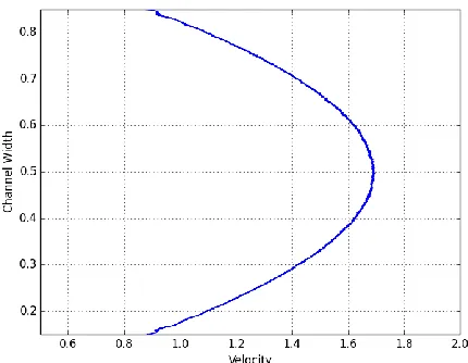
a) Density profiles of a fluid in a nanochannel.The walls of the channel are the thick, dark blue slabs on the top and bottom of the figure (where the density is zero since there are not liquid atoms there). The liquid density is not uniform. Instead, it

forms discrete, structured layers close and parallel to the channel walls.

b) Velocity profiles of flow in a nanochannel. It shows that at the solid-liquid interface, the velocity is not zero. This urges

reconsideration of the no-slip condition commonly used in continuum approaches.

Fig. 1.1 Density (a) and velocity profiles (b) of a liquid in a nanochannel.

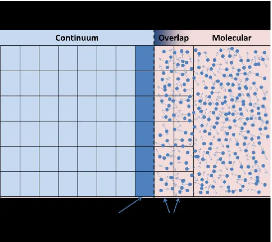
The main issue in atomic-scale simulations is the computational cost, which increases significantly with the size of the simulation domain. Hence, complications arise in micro-flows in which the non-homogeneities and interfacial effects of nano-flows are still evident, rendering continuum mechanics inadequate, yet the system size is outside the practical scope of MD.

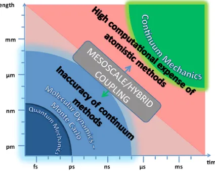
This blend of difficulties in such systems renders the independent use of either continuum or atomistic methods insufficient or practically impossible. To account for this, mesoscale and hybrid molecular-continuum methods (HMCM) have been of academic interest for over two decades now. These approaches attempt to bridge the two types of models into a synergy, which allows for an accurate calculation of the properties of the system at a relatively low computational cost. Mesoscale models comprise a single solver, which attempts to give a more efficient solution based on atomistic observations, while HMCM utilise both molecular and continuum solvers that exchange information. Fig. 1.2 shows the time and length scales in which quantum, atomistic, continuum and hybrid methods are used.

strengths and limitations of each method are also discussed. Section 4 discusses hybrid multiscale methods. As the name suggests, these utilise both, a continuum and a molecular solver to address different physical scales. We categorise these methods depending on how the system is decomposed into molecular and continuum components and how information is exchanged between the atomistic and continuum solvers.

Section 5 summarises the conclusions drawn from the present work.

Fig. 1.2 Time and length scales of computational methods for micro and nano fluids.

2

Computational Methods

2.1

Molecular Dynamics

MD is a deterministic computational method, which calculates the trajectory of all atoms in time. Given the atomic positions 𝒓 and velocities v, the system is evolved through Newton’s equations of motion

𝒓̇𝑖= 𝒗𝑖, 𝐹𝑖= 𝑚𝑖𝑣̇𝑖, 2.1

where the index 𝑖 represents and arbitrary particle (atom or molecule); and 𝑭𝑖 is the force acting on the particle,

determined by

𝑭𝑖= −∇𝒱 = − 𝜕

where 𝒱 is the total potential energy of the system, which depends on the relative positioning of all the atoms, as well as the nature of the intermolecular and intramolecular interactions in the system. An accurate description of this potential is within the scope of quantum electrodynamics. However, MD uses empirical functions that can

accurately portray the atomic interactions. A popular pairwise potential that MD simulations often use for non-bonded, van der Waals interactions is the Lennard-Jones (LJ) potential given by the function

𝑉𝐿𝐽_{= 4𝜀 [(}𝜎 𝒓)

12 + (𝜎

𝒓) 6

]

where 𝜀 is the depth of the potential well and 𝜎 is the point of intersection with the interatomic distance axis (Fig. 2.1). As Fig. 2.1 shows, at small interatomic distances, a strong repulsive force is acting on the two atoms, which tends to infinity as their separation approaches zero. This corresponds to the Pauli exclusion principle, which prevents the electron shells of the particles from overlapping. The blue-shaded region in the figure corresponds to the attractive London-dispersion forces acting between non-reacting gases such as argon.

Fig. 2.1 The Lennard-Jones potential. The red-shaded area corresponds to the strong repulsive forces, a product of the Pauli exclusion principle, whereas the blue-shaded area corresponds to the attractive London-dispersion forces.

Therefore, the objective of all mesoscale and multiscale approaches is to decouple the microscopic spatial and time scales from a large part of the domain, thus allowing the simulations to be performed within more realistic time scales.

2.2

Continuum Model

The continuum model does not treat systems as a collection of atomic trajectories. Instead, the primitive state variables such as density 𝜌, flow velocity 𝒖, energy 𝑒, temperature 𝑇 and pressure 𝑝, are considered as functions of time and space, averaged over a large number of atoms (e.g. 𝜌 = 𝜌(𝑥, 𝑦, 𝑧, 𝑡) in Cartesian co-ordinates).

The behaviour of fluids in this continuum approach is governed by the Navier-Stokes equations; a set of three equations based on the conservation of mass, momentum and energy, given by

𝜕𝜌

𝜕𝑡 = −∇. (𝜌 𝒖) 2.3

𝜕𝜌𝒖

𝜕𝑡 = −∇. (𝜌 𝒖⨂𝒖) − ∇. 𝚷 2.4 𝜕𝑒

𝜕𝑡 = −∇. (𝑒𝒖) − ∇. (𝚷. 𝒖) − ∇. 𝐪 2.5

where the stress tensor 𝚷 of a Newtonian fluid is empirically given by

𝚷 = p𝐈 − 𝝀𝒗(∇. 𝐮)𝑰 − 𝜇[(∇𝐮) + (∇𝐮)𝑻] 2.6

the heat flux vector 𝒒 is given by

𝒒 = 𝝀∇T 2.7

and the equations of state for 𝑝 and 𝑇 are given by

𝑝 = 𝑝(𝜌, 𝑒𝑖) and 𝑇 = 𝑇(𝜌, 𝑒𝑖) 2.8

3

Mesoscale Methods

In an attempt to bridge the microscopic and macroscopic environments, mesoscale methods provide a framework of intermediate resolution. They are based on the often correct assumption that the behaviour of every single atom is not required to produce realistic results. Instead, large numbers of molecules are grouped together. Within the scope of mesoscale methods, these pseudo-particles are considered fundamental and interact among themselves without considering the influence of their constituent atoms.

3.1

Lattice Gas Automaton

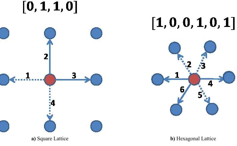
the representation of each lattice point by a Boolean vector with a dimension equal to the number of possible directions (i.e. lattice links) from each node. For each direction, the value is 1 if there is an atom on that point moving with that velocity.

In order to illustrate the above, Fig. 3.1a shows one possible configuration of atoms (chosen arbitrarily) found on a lattice site (the red circle) on a square lattice. The arrows indicate the possible values of the velocity. A solid line means that an atom moving in that direction is located on the lattice point while a dotted line suggests that such an atom is absent. Since the velocity can take four values, a four-dimensional vector is used to describe the state of the node. Since there is no atom moving in direction 1 and 4 (suggested by the dotted lines in those directions), the corresponding components in the vector are 0. On the other hand, the third and fourth components have a value of one indicating that there are two atoms moving in directions 3 and 4.

At each time step, LGA carries out two operations:

1. Propagation. During this step, the particles are moved to nearby lattices depending on their velocities of the previous time step. For example, in Fig. 3.1a the atom with velocity 2 will move to the top vertex, pointed by the arrow, in the next time step. As we have mentioned earlier in this section, two atoms located at the same point cannot move along the same direction.

a) Square Lattice b) Hexagonal Lattice

Fig. 3.1 Boolean representation of a lattice point (red node) a) for a square lattice and b) for a hexagonal lattice. The arrows indicate the possible velocities. A solid line suggests that the red lattice site has an atom moving in that direction

while a dashed line indicates that there is no particle with that velocity on that point.

This seemingly simplistic model can potentially reproduce the Navier-Stokes equations by taking averages over a large number of nodes. This, however, requires a lattice with sufficient symmetry. The four-fold symmetry of the lattice depicted in Fig. 3.1a is incapable of reproducing the hydrodynamic equations. For two-dimensional systems, the symmetry of the hexagonal lattice illustrated in Fig. 3.1b is indeed sufficient. Such a system allows the atoms to move in six directions. To accommodate this, we require six-dimensional vectors to store the state of each lattice point at each time step. In addition, more collision rules are required as particles can now collide at more angles. Hydrodynamic lattices are also available for three-dimensional systems.

Finally, it is worth mentioning the key differences between MD and LGA since both methods consider interacting particles. MD is grid-less and therefore does not restrict the motion of atoms. Additionally, as we have mentioned in section 2.1, MD considers microscopic interactions, which classically approximate quantum mechanical behaviour as accurately as possible. This gives rise to realistic equations of state whereas the collision rules of LGA only facilitate isothermal relationships between mass, density and pressure. However, the simplicity of LGA models is accompanied by a very attractive computational efficiency, which is of course the objective of multiscale models.

3.2

Lattice-Boltzmann Method

only have an integer value. Averaging over a large number of nodes can reduce this noise but costs computationally. The Lattice-Boltzmann (LB) method, (McNamara & Zanetti, 1988; Chen & Doolen, 1998) attempts to resolve these issues by storing the real particle density at each lattice point. Furthermore, although the particles can travel along the lattice directions, as in LGA, a real number of particles on each lattice site occupy each of them. Therefore, the density and velocity of the fluid at a certain position along a certain direction are given by

𝜌(𝒙) = ∑ 𝑓𝑖(𝒙) 𝑖

3.1

𝑢(𝒙) = ∑ 𝑓𝑖(𝒙)𝒄𝑖 𝑖

3.2

where 𝒙 is the lattice point, 𝑖 is an arbitrary lattice direction, 𝑓𝑖(𝒙, 𝑡) is the portion of the density of the lattice site

moving in a lattice direction and 𝒄𝑖 is the corresponding lattice vector.

As in the LGA models, the evolution of the system consists of a propagation and collision step. The propagation step is given by

𝑓𝑖(𝒙 + 𝒄𝑖∆𝑡, 𝑡 + ∆𝑡) = 𝑓𝑖(𝒙, 𝑡)

simply stating that the density distribution in a certain direction at a node inherits that of its neighbour (along the vector 𝒄𝑖) from the previous timestep. Accounting for collisions, the full equation becomes

𝑓𝑖(𝒙 + 𝒄𝑖∆𝑡, 𝑡 + ∆𝑡) − 𝑓𝑖(𝒙, 𝑡) = Ω𝑖(𝑓) 3.3

where Ω is the collision operator and 𝒄𝑖 are the lattice-restricted velocities.

Due to the additional complexity of LB models in comparison with LGA, more complicated collision operators are required. This is usually approximated by the Bhathagar-Gross-Krook (BGK) operator given by (Bhatnagar, 1954)

Ω: 𝑓𝑖→ − 1

𝜏[𝑓𝑖− 𝑓𝑖𝑒𝑞] 3.4

where 𝑓_𝑖𝑒𝑞 is the equilibrium particle distribution based on the discretized version of the Maxwell-Boltzmann equilibrium distribution (Qian, 1992).

LBM can also treat physical phenomena where body forces are involved. Such cases include multi-phase and multi-component systems. This, however, requires the addition of the force to the evolution equation (Eq. 3.3) and that the velocity and equilibrium distribution are adjusted accordingly (Guo et al., 2002).

The base model described above can be modified to accommodate various flow phenomena. For Poisseuille flow, the collision rules at the solid-liquid interface are adapted so that fluid particles arriving at the boundary are bounced back by inverting the lattice velocity (Succi, 2001). For Couette flow, this model is adjusted so that part of the boundary momentum is injected into the bounced fluid (Ladd, 1994). This approach models the boundaries at lattice link midpoints and is therefore unable to capture the behavior of arbitrarily curved surfaces. Subsequent studies have proposed extensions to these models to account for more complex geometries (Filippova, 1998; Guo et al., 2002)

The method also enables simulations of complex, and multi-phase flows by modelling potential interactions between the pseudo-particles. This is achieved by defining an external force, which acts on 𝑓𝑖𝑒𝑞. The mesoscale

interactions can naturally give rise to non-ideal fluid. This allows for simulation of complex systems such as the effect of gas bubbles on the liquid slippage at a rough solid surface (Hyvaluoma & Harting, 2008). To realise such effects, the free-energy functional of the system is considered, giving rise to a pressure tensor that can be included in

𝑓𝑖𝑒𝑞 (Swift et al., 1995).

An alternative method is to include an interaction term between the pseudo-particles, given by (Shan & Chen, 1994)

𝐹(𝑥) = 𝜓(𝒙) ∑ 𝑔𝑖𝐺𝜓(𝒙 + 𝜓(𝒙 + 𝒄𝒊)𝒄𝒊) 𝑖

3.5

where 𝐺 is the ratio of the potential and thermal energy, 𝜓(𝒙) is the potential that describes the interactions of the pseudo-particles under inhomogeneities and 𝑔𝑖 is a lattice-dependent weighting factor dividing the force among the

various lattice directions. Adjusting the equilibrium distributions based on the effects of this force on the velocity provides an equation of state, which for high values of 𝐺 resembles the van der Waals equation, enabling the simulation of liquid-gas interfaces. Although the thermodynamic validity of this pseudo-potential scheme has been criticised as it is not derived from a free-energy functional, it has been proven effective in successfully describing various systems. Furthermore, the addition of a gradient force in Eq. 3.5 can bridge these thermodynamic inconsistencies (Sbragaglia et al., 2009).

3.3

Dissipative Particle Dynamics

Dissipative particle dynamics (DPD) is a mesoscale approach in which, unlike LGA and LB, pseudo-particles move continuously in space rather than jumping across points on a lattice (Hoogerbrugge & Koelman, 1992). These bodies represent groups of atoms or sub-thermodynamic ensembles and interact among themselves through pairwise interactions. In this sense, DPD can be considered as a coarse-grain equivalent of MD. Each pseudo-particle moves in free space. Its momentum is updated every time step according to the force acting on it given by

𝐹𝑖= ∑(𝐹𝑖𝑗𝐶+ 𝐹𝑖𝑗𝐷+ 𝐹𝑖𝑗𝑅)

𝑖≠𝑗 3.6

The term 𝐹𝑖𝑗𝐶 is a purely repulsive, conservative force that prevents major overlaps between the particles. This

component acts in the same way as the repulsive component of the non-bonded potentials that MD employs (e.g. Lennard Jones potentials). However, the more complicated potentials of microscopic simulations produce forces that increase to infinity as the interatomic distance approaches zero. As we have mentioned in section 2.1, this severely restricts the maximum timestep that can be used. However, if we average these interactions over large groups of atoms, such as in DPD, a “softer” potential can be used which is finite even at zero separation. This allows the use of a much larger time step, a very attractive quality of this mesoscale method that allows the simulation of more practical systems. The dissipative (𝐹𝑖𝑗𝐷) force describes viscous, frictional forces and it is a function of interatomic

distances and relative velocities between atoms in the system. Finally, the term 𝐹𝑖𝑗𝑅 is a stochastic force that

atomic fluctuations within the pseudo-particles) of these mesoscale particles and regulate the temperature (they act as a Langevin thermostat). Once the force is defined, Newton’s second law of motion (Equation 2.1) is used for advancing the trajectory of the system through phase space. The conservative force is then given by

𝐹𝑖𝑗𝐶 = 𝑎𝑖𝑗𝑤𝐶(𝑟)𝒓𝑖𝑗 3.7

where 𝑎𝑖𝑗 is the maximum repulsion between the dissipative particle 𝑖 and 𝑗, 𝑟 is their interatomic distance, and 𝑤𝐶_{(𝑟) is a weight function, often set to}

𝑤𝐶_{(𝒓) {(1 − 𝑟) 𝑟 < 1.0}

0 𝑟 ≥ 1.0 3.8

This formulation only includes a repulsive component. Although this is an accurate approximation of gases, for more complex systems such as multi-phase flow an attractive component should also be added. In this case, the weight function can be given by (Liu et al., 2006; Liu et al., 2007)

𝑤𝐶_{(𝒓) = −[𝐴𝑊′}

1(𝑟, 𝑟𝑐1) − 𝐵𝑊′2(𝑟, 𝑟𝑐2)] 3.9

where 𝑊1(𝑟, 𝑟𝑐1) and 𝑊2(𝑟, 𝑟𝑐2) are spline functions representing the repulsive and attractive interactions; 𝐴 and 𝐵

define their strengths; and 𝑟𝑐1 and 𝑟𝑐2 are their cut-off distances.

4

Hybrid Molecular-Continuum Methods

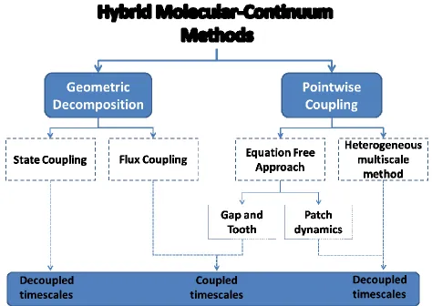
Fig. 4.1 General classification of. Hybrid Molecular-Continuum Methods (HMCM) Geometric decomposition and pointwise coupling differ with respect to the implementation of the molecular and continuum solvers in the simulation

box.

An alternative method for dealing with systems at microscales is the the Hybrid Molecular-Continuum Methods (HMCM) in which both molecular (usually MD or MC) and continuum (usually CFD and FEM) solvers are used (Kalweit & Drikakis, 2011). The basic principle behind these hybrid techniques is to limit the use of the molecular solver as much as possible. The size of the domain (i.e., number of atoms) is the biggest bottleneck in molecular methods. Therefore, all HMCM decouple the length scales by running molecular simulations in one or more subdomains, small relative to the overall size of the system. In addition, some HMCM decouple the timescales by running the molecular simulations for only selected periods. Fig. 4.1 illustrates a general categorisation of the available HMCM. Geometric decomposition and pointwise coupling are based on how the model allocates the system to the molecular and continuum solvers. Geometric decomposition divides the system spatially and

them decouple the macroscopic and microscopic timescales. Note that employing equilibrium kinetic theory

concepts to what is definitely a non-equilibrium process should be borne in mind when considering the limitations of multiscale methods. Although this is recognised by the present authors, it is an issue that requires further elaboration that is beyond the scope of the present study. The aforementioned methods are discussed in more detail below.

4.1

Geometrical Decomposition

Geometrical decomposition (GD) refers to a HMCM in which the simulation domain is decomposed into regions, some of which are dealt with by the molecular and others by the continuum solver. As the objective of such hybrid methods is to minimise computational resources, the higher resolution molecular regions should be much smaller than the continuum regions.

The continuity of thermodynamic and transport properties between the various parts of the system is integral in modelling a physically accurate environment. It is therefore crucial to define a protocol in which the two solvers share information with each other and adjust in order to conform to the laws of physics. This is achieved by defining an overlapping region near the interface of the two regions, called Hybrid Solution Interface (HSI), which is treated both by the continuous and molecular components.

Fig. 4.2 depicts the process behind GD. The continuum region on the left, highlighted in light blue, is solved using a finite volume method and is therefore divided into cells. The grid is extended slightly into the molecular domain. The coinciding cells are called ghost cells. Although the domain in molecular methods is not traditionally divided into a grid, virtual cells are defined which coincide with the ghost cells of the continuum solver. This sets up a framework enabling the exchange of information between the two.

The coupling of the solvers is bidirectional. The molecular component calculates properties within the virtual cells and imposes them onto the ghost cells. In turn, these will adjust the boundary cells (dark blue cells in Fig. 4.2). On the other hand, macroscopic properties in the ghost cells are imposed onto the molecular domain by adjusting the number and velocities of the atoms within the corresponding virtual cells.

The protocol at the HSI varies significantly between GD implementations. However, all GD schemes need to satisfy a set of fundamental requirements; namely:

 The conservation laws of mass, momentum and energy should hold across the boundary.

 The state variables across the boundary must portray a physically accurate behaviour. This means that by looking at the flow solution of the simulation (i.e. density profiles), the position of the HSI should not be identifiable.

The coupling must be also designed in the most simplistic and computationally efficient manner possible. GD can differ in the type of information used for coupling the two solvers. Two broad categories can be identified

1. State Coupling 2. Flux Coupling

Fig. 4.2 Schematic representation of GD.

4.1.1 State-Coupling

State coupling refers to the sharing of state variables such as density, temperature and velocity, across the HSI. Fig. 4.3 illustrates a one-dimensional setup for coupling by states with the continuum region being on the left and the molecular region on the right. The vertical separation is merely an artefact to aid in the visual clarity of the figure.

Fig. 4.3 A one-dimensional illustration of coupling by states in both directions. The continuum and molecular domains are separated to aid visualisation. The arrows symbolise the transfer of states from the continuum to the

molecular domain (C->M) and vice versa (M->C).

macroscopic quantities can be obtained through spatial and temporal averaging of the atomic behaviour. In general, a state variable 𝒜 has an instantaneous value, obtained by averaging the behaviour of many atoms at an arbitrary instance. As a statistical quantity, this value can fluctuate significantly across different points in time. The reduction of these fluctuations is achieved through averaging the instantaneous calculations over a suitably long timescale by:

〈𝒜〉𝑡= 1

𝛿𝑡 ∫ 𝒜(𝑡)𝑑𝑡, 𝑡0+𝛿𝑡

𝑡₀

4.1

where 〈𝒜〉𝑡 denotes the time average of the quantity 𝒜; 𝑡0 denotes the initial timeframe in which the value is

calculated; 𝛿𝑡 is the timescale over which the quantity is averaged; and 𝒜(𝑡) is the instantaneous calculation. For computational purposes, the equation can be written in discrete form as

〈𝒜〉𝑡= 1

𝑁𝑡∑ 𝒜(𝑡) 𝑁_𝑡

𝜏=0

, 4.2

where 𝜏 denotes the timestep of the molecular simulation and 𝑁𝑡 is the number of timesteps used for the averaging.

The ghost and boundary cells can trivially inherit the calculated values.

Transferring information from the continuum to the molecular domain is a more complicated task. The difficulty arises from the requirement to construct a microscopic state of 6𝑁 degrees of freedom (momentum and position of 𝑁 atoms) from the macroscopic state, with only 5 degrees of freedom (𝜌, 𝒖 and 𝑒) (Asproulis et al., 2009). This interpolation requires additional assumptions or stochastically generated values.

For incompressible flows, this is achieved by matching the atomic number density and average velocity in the HSI with the corresponding continuum values. Inserting or deleting atoms in the virtual cells controls the density. The momentum is coupled by rescaling the atomic velocities accordingly. The temperature can also be regulated based on the equipartition theorem, according to the equation

𝑇 = 2

3𝜅𝐵𝑒̅̅̅𝑘 4.3

where 𝑒̅̅̅𝑘 is the average kinetic energy of all atoms about their mean position, i.e., excluding the kinetic energy of

the center of mass within that cell and 𝜅𝐵 is the Botlzmann constant.

State coupling becomes much more complicated for compressible flows as the positions and momenta of the atoms must also match the continuum energy. Although in its own right this is not a difficult task, the abundance of microscopic states fulfilling this constraint must further be reduced to those maximising the entropy of the system and, in turn, satisfy the second law of thermodynamics. Such a task greatly increases the computational complexity of the algorithm, a highly undesirable outcome.

simulation box with periodic boundary conditions serving as a particle reservoir. More recent advances in state coupling, MD-CFD methods emulated mass flow by inserting and deleting particles that cross the HSI (Werder et al., 2005). The model has been used to study flow of a Lennard-Jones fluid around a Carbon Nanotube (CNT) the results of which agreed with those similar cases treated exclusively with MD. State-coupling methods suitable for unsteady flows have also been derived (Liu et al., 2008).

Methods for reducing the noise resulting from the thermal fluctuations in the molecular domain have also been proposed (Ko et al., 2014). This has been achieved by sampling the state variables from multiple, replicated molecular systems set at different initial conditions. Furthermore, by spatial and temporal regressions, a more accurate exchange of variables can be achieved.

4.1.2 Flux Coupling

Rather than exchanging information on the state of each region, flux coupling methods update the state variables by monitoring the inflow and outflow of mass, momentum and energy. The monitoring is required to account for all ways in which quantities can be transported. Mass can only be transferred through convection; the bulk motion of fluid particles. Momentum can be transferred by both convection and the stresses applied on atoms by their neighbours. Finally, energy can be transferred by convection, through interatomic stresses, as well as through conduction.

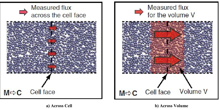
As in the case of state coupling, the transfer of information from the molecular to the continuum domain is simpler than the inverse exchange (continuum to molecular). We achieve this by monitoring and calculating the flow of a quantity through a virtual cell face within the overlapping region or an arbitrary volume enclosing the surface. This flow can then be imposed on the corresponding ghost cells (or corresponding volume enclosing the ghost cell’s face). This can be seen in Fig. 4.4 where the vertical, black, dashed line indicates the face of the cell. Fig. 4.4a illustrates that the flux is measured by the rate in which atoms or molecules cross this surface. In Fig. 4.4b, the shaded red region is the volume containing the surface, in which the fluxes are calculated. Once the atomic

a) Across Cell b) Across Volume Fig. 4.4 Schematic representation of Flux coupling.

The exchange of fluxes from the continuum to the molecular domain is again more complicated as the fluxes in and out of the ghost cells must be mapped onto the virtual cells. To account for convective fluxes, atoms are inserted or deleted in the virtual cells of the HIS. The number of atoms regulates the mass transfer, and their velocities control the convective momentum and energy transfer. In order to impose momentum transfer through stress, appropriate force fields are applied onto the atoms. Finally, the conductive flux can be realised by rescaling the velocities of the atoms, emulating energy transfer.

Incompressible, isothermal flows are significantly simpler than compressible cases as the two energy fluxes (stress and conductive) can be ignored (Hadjiconstantinou & Patera, 1997; Barsky, 2004; De Fabritiis, 2007). However, all fluxes can be incorporated into the molecular domain, allowing for the simulation of compressible flows (Delgado-Buscalioni & Coveney, 2003a). Additionally, this method is suitable for phenomena whose characteristic time scales are comparable to molecular time scales, such as waves (Delgado-Buscalioni, 2005; De Fabritiis, 2007). However, due to the constant need to monitor the fluxes across the molecular and continuum regions, GD flux coupling methods do not decouple timescales and are, therefore, not preferred by some authors (Wijesinghe & Hadjiconstantinou, 2004; Koumoutsakos, 2005).

polymer in a solvent, subjected to oscillatory flow (Barsky, 2004). Past studies have investigated the boundary conditions used in the flux coupling approaches attempting to smoothen any numerical artifacts and discontinuities induced at the HSI (Kalweit & Drikakis, 2008a; Kalweit & Drikakis, 2008b; Kalweit & Drikakis, 2010). Extensions to the flux coupling models have been proposed to take into account the fluctuations of state variables when transferring information from the molecular to the continuum region. This can be achieved by adapting the macroscopic equations as well as by implementing a relatively fine grid near the HSI. Such flux coupling methods have successfully simulated sound waves propagating through water and reflected by a lipid monolayer (Delgado-Buscalioni, 2005; De Fabritiis, 2007). Previous investigations have also used GD to couple fluxes from the continuum to the molecular domain in connection with the study of dynamic friction between crystal silver on copper at high pressure (Barton et al., 2011).

4.2

Pointwise Coupling

Rather than having regions treated exclusively by a molecular or continuum solver (as is the case with GD), the pointwise coupling (PWC) solves the entire domain using the continuum solver, with the molecular component acting as a refinement by providing information used for more accurate calculations (Asproulis et al., 2012). There are two types of problems in which such methods are effective:

a) Problems in which the boundary conditions (e.g. velocity slip) need to be resolved by the microscopic solver;

Fig. 4.5 A schematic illustration of length decoupling in PWC.

The entire domain is solved by the continuum model (blue), while the microscopic solver is used at specific grid points (red) to assist the macroscopic solution. Several PWC based coupling methods (for both solids and fluids) have been proposed based on the above description. These differ in the involvement of the molecular solver and the means by which the properties in question are computed and can be generalised into two categories.

1. Heterogeneous multiscale Method 2. Equation-free approach

a. Patch dynamics b. Gap-tooth method

Fig. 4.6 A schematic illustration of length decoupling in PWC. For coupled timescales, the molecular and continuum simulations run in parallel. For decoupled timescales the molecular simulation runs for a number of microscopic time

steps at specific macro time steps.

4.2.1 Heterogeneous Multiscale Method

The heterogeneous multiscale method (HMM) (Enguist & others, 2003) assumes knowledge of the physical, continuum equations required for the calculation and evolution of the flow field. As the macroscopic field is not explicitly known across the entire domain, there is often a lack of data essential for the solution of these equations, e.g., stress tensor. The microscopic solver provides the relevant information.

For modelling the physical system, the following should be considered  The continuum model to be used.

 The data computed by the microscopic solver to be fed into the macroscopic model.

 Conversion of a continuum state into a consistent microstate (as explained in the Section 4.1.1).  Conversion of averaging a microstate to realise the continuum value.

The system is then advanced based on the following steps

1. From a macroscopic state variable 𝑈, the microstate is reconstructed by adjusting the positions and momenta of the atoms.

2. Using the molecular solver, the system is evolved and the necessary data (usually stress tensor or slip condition) is computed.

3. The data are then inserted into the macroscopic model to realise the field at a later time

Initial implementations of HMM have successfully simulated phenomena such as homogenisation, dislocation dynamics and crack propagation (Weinan et al., 2003). Subsequent studies have used such methods to model complicated flows, e.g., driven cavity flows (Ren & Weinan, 2005). MD was used to calculate the stress tensor from first principles, using the Irving-Kirkwood formula, instead of relying on assumptions that are inaccurate

polymeric fluids. Traditional formulation of HMM is unable to study steady-state problems since the velocity field

𝑈, used to impose boundary conditions on the molecular solver, vanishes along with the time derivative in equation 2.4. Recent studies have circumvented this problem by using the Laplacian of the streaming velocity and

temperature (Alexiadis et al., 2013) to calculate momentum and heat transfer. In addition, their method avoids using the complicated Irving-Kirkwood equations to calculate the stress tensor and, instead, uses the simpler ‘framed’ cell approach (Hadjiconstantinou & Patera, 1997; Massarotti et al., 2010). The approach was validated by simulating a flow through a channel under the effect of gravity.

A variation of the HMM, is the Internal-flow Multiscale Method (IMM), tailored for micro and nanoflows through channels of high aspect ratios. The system is again treated entirely by the continuous solver. However, the microscopic component treats thin strips across the entire width of the channel rather than small regions around grid points. The rationale is that for very narrow channels, the molecular regions of traditional HMM which need to have a minimum volume (depending on the mean free path of the system), might overlap introducing a computational overhead surpassing the computational expense of full MD. Rather than imposing the velocity field onto the molecular region, IMM imposes pressure gradient, emulated through an applied force.

Fig. 4.7 Schematic representation of IMM. The entire channel is solved with a continuum solver. The molecular component is used over sparsely placed, thin regions, spanning the entire width of the channel.

Recent studies have introduced the field-wise coupling (FWC) approach (Borg et al., 2013a), circumventing the limitation of traditional HMM methods in relatively coarse grids.. In contrast to PWC that couples the molecular region to a node of the continuum grid, FWC couples the MD and CFD regions. MD simulations are used to calculate stress and velocity profiles within molecular domain, and feed their values into the CFD solver. The microscopic elements can have an arbitrary position and size, hence increasing the versatility of the method for different characteristic system dimensions and enabling flow phenomena of varying length scales to be modelled. The HMM-FWC approach in conjunction with DSMC was also extended to model heat transfer problems in rarefied gases (Docherty et al., 2014).

To further improve the computational efficiency of PWC models, MD calculations can be cached into suitable data structures for use at a later timestep (Asproulis & Drikakis, 2013). If the information requested by the

continuum model resembles previously processed data, then the molecular result is extracted from the cache, rather than requiring re-computing. Furthermore, artificial neural networks can be trained to optimise the volume of stored information and to minimise the molecular fluctuations.

4.2.2 Equation-Free Approach

The Equation-Free Approach (EFA) is a PWC method, which circumvents the need for continuum closed form equations (Kevrekidis et al., 2003; Kevrekidis et al., 2004). The main idea is that small bursts of appropriately initialised microscopic simulations can be used to calculate the same information that explicit continuum formulas would produce. The gap-tooth method defines small regions (referred to as “teeth”) in space where the microscopic solver calculates desired observation variables (e.g. density) (Gear et al., 2003). Spatial interpolation between the calculations of these regions can compute the macroscopic field. This successfully decouples the microscopic and macroscopic spatial scales but does nothing to decouple the time between them.

Patch dynamics can then be used to decouple timescales. In general, given the initial value of a property 𝑐, marked as 𝑐0, as well as its time derivative 𝑑𝑐_𝑑𝑡, one can use the forward Euler method

𝑐𝑛+1= 𝑐𝑛+ τ 𝑑𝑐

𝑑𝑡 4.4

to calculate the value of 𝑐 at future times. Here, τ is the macroscopic timestep. Although a model would normally be used for the derivative, the patch dynamics approach calculates it by allowing the microscopic solver to run for a small period of time. We can then project the solution to the next macroscopic timestep τ using the forward Euler method (or more generally a Taylor series). During this macroscopic timestep, the molecular solver is not used at all. However, following the projection step, the microscopic simulation must be re-initialised accordingly to obtain the derivative for the next iteration. Since the molecular component runs for a short period of time, following the macroscopic timestep, the patch dynamics approach also decouples the macro and micro timescales.

The macroscopic and microscopic timestep used for the EFA can vary significantly depending on the problem to be modelled and the computational method employed. In fact, this approach is by no means restricted to a specific type of microscopic model. Many applications have used mesoscale models to compute the field in between

arrays of bubbles in a two-phase liquid (Sankaranarayanan et al., 2002; Sankaranarayanan et al., 2003;

Theodoropoulos et al., 2004). The EFA, in conjunction with the LBM, has also been used to study reaction-diffusion problems (Kevrekidis et al., 2003). Investigations have also used patch dynamics with kinetic Monte Carlo to study a model of heterogeneous catalytic surface reactions (Makeev et al., 2002; Siettos et al., 2003).

Although the above investigations have demonstrated that this method is effective, it is usually restricted to problems where the macroscopic physics are not well understood. In the case where continuum, closed-form equations are available, HMCM such as GD or HMM are preferred.

5

Conclusions

The recent academic and industrial interest in micro and nanofluidic devices has necessitated the development of computational strategies that can assist the design of such devices. From the perspective of the physical

understanding of such systems, the high-resolution molecular methods are ideal approaches. Their computational cost, however, significantly limits their use to systems containing a modest number of atoms. For larger scales, the computational efficiency of continuum methods such as CFD is particularly appealing but the steep gradients and discontinuities characterising microflows are beyond the scope of the Navier-Stokes equations.

This review presented the efforts for the design of computational models attempting to bridge the gap between accuracy and computational efficiency. Various mesoscale models, which provide an intermediate resolution for computation, and hybrid methods, which use both molecular and continuum solvers for the description of the fluid field were presented. To date, there is no universal method, which covers all regimes. The appealing simplicity of the LGA is compromised by the discrete nature of the velocities and density, which produces unrealistic physical phenomena for complex systems. Although the more refined LBM has been improved significantly over the years to include various effects, e.g. multi-phase flows, boundary conditions, disadvantages emerging from the limitation of lattice-based system dynamics, still exist. As a coarse-grained version of MD, DPD is an appealing method with the capability of providing an accurate representation of complex systems. However, depending on the grouping of the molecules, the dissipative pseudo-particles, interatomic and intermolecular interactions can be blurred.

HMCM provide a good comprise by using both solvers. Complications arise, however, in the choice of the regions in which the molecular solver will be applied. GD for example, might not be appropriate in systems, where the entire channel is governed by microscopic phenomena and, therefore, the definition of a continuum region is not possible without compromising accuracy. PWC based approaches generally seem to be the most versatile,

potentially providing information across the entire domain. However, when the geometries and gradients vary significantly within small length scales the number of molecular regions needs to increase, which can quickly add to the overall computational expense.

Finally, although significant advances in multiscale modelling are yet to be made, the efforts of the last three decades have facilitated a number of options, which can be considered for a large spectrum of flow regimes of interest in engineering.

Compliance with Ethical Standards

We confirm that there are no potential conflicts of interest or research involving Human Participants and/or Animals.

6

Bibliography

Alexiadis, A., Lockerby, D.A., Borg, M.K. & Reese, J.M., 2013. A Laplacian-based algorithm for non-isothermal atomistic-continuum hybrid simulation of micro and nano-flows. Computer Methods in Applied Mechanics and Engineering, 264, pp.81--94.

Allen, M.P. & Tildesley, D.J., 1989. Computer simulation of liquids. Oxford: Oxford university press. Asproulis, N. & Drikakis, D., 2010. Boundary slip dependency on surface stiffness. Physical Review E, 81, p.061503.

Asproulis, N. & Drikakis, D., 2011. Wall-mass effects on hydrodynamic boundary slip. Physical Review E, 84, p.031504.

Asproulis, N. & Drikakis, D., 2013. An artificial neural network-based multiscale method for hybrid atomistic-continuum simulations. Microfluidics and Nanofluidics, 15, pp.559--574.

Asproulis, N., Kalweit, M. & Drikakis, D., 2012. A hybrid molecular continuum method using point wise coupling. Advances in Engineering Software, 46(1), pp.85--92.

Asproulis, N., Kalweit, M., Shapiro, E. & Drikakis, D., 2009. Mesoscale flow and heat transfer modelling and its application to liquid and gas flows. Journal of Nanophotonics, 3(1), pp.031960-60.

Baranyai, A., Evans, D.J. & Daivis, P.J., 1992. Isothermal shear-induced heat flow. Physical Review A, 46, p.7593.

Barrat, J.-L. & Chiaruttini, F., 2003. Kapitza resistance at the liquid—solid interface. Molecular Physics, 101, pp.1605--1610.

Barsky, S.a.D.-B.R.a.C.P.V., 2004. Comparison of molecular dynamics with hybrid continuum--molecular dynamics for a single tethered polymer in a solvent. The Journal of chemical physics, 121, pp.2403--2411.

Barton, P., Kalweit, M., Drikakis, D. & Ball, G., 2011. Multi-scale analysis of high-speed dynamic friction.

Journal of Applied Physics, 110(9), p.093520.

Bhatnagar, P.L.a.G.E.P.a.K.M., 1954. A model for collision processes in gases. I. Small amplitude processes in charged and neutral one-component systems. Physical Review, 94(3), p.511.

Bitsanis, I., Magda, J., Tirrell, M. & Davis, H., 1987. Molecular dynamics of flow in micros. The Journal of chemical physics, 87, pp.1733--1750.

Borg, M.K., Lockerby, D.A. & Reese, J.M., 2013b. A hybrid molecular-continuum simulation method for incompressible flows in micro/nanofluidic networks. Microfluidics and nanofluidics, 15, pp.541--557.

Chen, S. & Doolen, G.D., 1998. Lattice Boltzmann method for fluid flows. Annual review of fluid mechanics, 30(1), pp.329-64.

Choi, C.-H., Westin, K.J.A. & Breuer, K.S., 2003. Apparent slip flows in hydrophilic and hydrophobic microchannels. Physics of Fluids, 15, pp.2897--2902.

De Fabritiis, G.a.S.M.a.D.-B.R.a.C.P., 2007. Fluctuating hydrodynamic modeling of fluids at the nanoscale.

Physical Review E, 75, p.026307.

De Fabritiis, G., Delgado-Buscalioni, R. & Coveney, P.V., 2004. Energy controlled insertion of polar molecules in dense fluids. The Journal of chemical physics, 121, pp.12139--12142.

Delgado-Buscalioni, R.a.F.E.a.C.P., 2005. Fluctuations and continuity in particle-continuum hybrid simulations of unsteady flows based on flux-exchange. Europhysics Letters, 69, p.959.

Delgado-Buscalioni, R. & Coveney, P., 2003a. Continuum-particle hybrid coupling for mass, momentum, and energy transfers in unsteady fluid flow. Physical Review E, 67, p.046704.

Delgado-Buscalioni, R. & Coveney, P., 2003b. USHER: an algorithm for particle insertion in dense fluids. The Journal of chemical physics, 119, pp.978--987.

Delgado-Buscalioni, R. & Coveney, P.V., 2004. Hybrid molecular-continuum fluid dynamics.

PHILOSOPHICAL TRANSACTIONS-ROYAL SOCIETY OF LONDON SERIES A MATHEMATICAL PHYSICAL AND ENGINEERING SCIENCES, 362, pp.1639--1654.

Docherty, S.Y., Borg, M.K., Lockerby, D.A. & Reese, J.M., 2014. Multiscale simulation of heat transfer in a rarefied gas. International Journal of Heat and Fluid Flow, 50, pp.114--125.

Doerr, A., Tolan, M., Seydel, T. & Press, W., 1998. The interface structure of thin liquid hexane films. Physica B: Condensed Matter, 248, pp.263--268.

Enguist, B. & others, 2003. The heterogeneous multi-scale methods. Communications in Mathematical Sciences, 1, pp.87--133.

Filippova, O.a.H.D., 1998. Grid refinement for lattice-BGK models. Journal of Computational Physics, 147(1), pp.219--228.

Flekkoy, E.a.W.G. & Feder, J., 2000. Hybrid model for combined particle and continuum dynamics.

Europhysics Letters, 52, p.271.

Gear, C.W., Li, J. & Kevrekidis, I.G., 2003. The gap-tooth method in particle simulations. Physics Letters A, 316(3), pp.190--195.

Guo, Z., Zheng, C. & Shi, B., 2002. An extrapolation method for boundary conditions in lattice Boltzmann method. Physics of Fluids, 14(6), pp.2007--2010.

Guo, Z., Zheng, C. & Shi, B., 2002. Discrete lattice effects on the forcing term in the lattice Boltzmann method.

Physical Review E, 65(4), p.046308.

Hadjiconstantinou, N.G. & Patera, A.T., 1997. Heterogeneous atomistic-continuum representations for dense fluid systems. International Journal of Modern Physics C, 8, pp.967--976.

Hardy, J., Pomeau, Y. & De Pazzis, O., 1973. Time evolution of a two-dimensional model system. I. Invariant states and time correlation functions. Journal of Mathematical Physics, 14(12), pp.1746-59.

Henderson, J. & van Swol, F., 1984. On the interface between a fluid and a planar wall: theory and simulations of a hard sphere fluid at a hard wall. Molecular Physics, 51, pp.991--1010.

Hoogerbrugge, P. & Koelman, J., 1992. Simulating microscopic hydrodynamic phenomena with dissipative particle dynamics. EPL (Europhysics Letters), 19(3), p.155.

Hyvaluoma, J. & Harting, J., 2008. Slip flow over structured surfaces with entrapped microbubbles. Physical review letters, 100(24), p.246001.

Izquierdo, S., Martinez-Lera, P. & Fueyo, N., 2009. Analysis of open boundary effects in unsteady lattice Boltzmann simulations. Computers & Mathematics with Applications, 58(5), pp.914--921.

Jones, J.L., aNoel Ruddock, J., Spenley, N.A. & others, 1999. Dynamics of a drop at a liquid/solid interface in simple shear fields: a mesoscopic simulation study. Faraday Discussions, 112, pp.129--142.

Kalweit, M. & Drikakis, D., 2008a. Coupling strategies for hybrid molecular—continuum simulation methods.

Proceedings of the Institution of Mechanical Engineers, Part C: Journal of Mechanical Engineering Science, 222, pp.797--806.

Kalweit, M. & Drikakis, D., 2008b. Multiscale methods for micro/nano flows and materials. Journal of Computational and Theoretical Nanoscience, pp.1923--1938.

Kalweit, M. & Drikakis, D., 2010. On the behaviour of fluidic material at molecular dynamics boundary conditions used in hybrid molecular-continuum simulations. Molecular Simulation, 36(9), pp.657-62.

Kalweit, M. & Drikakis, D., 2011. Multiscale simulation strategies and mesoscale modelling of gas and liquid flows. IMA journal of applied mathematics, 76(5), pp.661-71.

Kevrekidis, I.G., Gear, C.W. & Hummer, G., 2004. Equation-free: The computer-aided analysis of complex multiscale systems. AIChE Journal, 50(7), pp.1346--1355.

Kevrekidis, I.G. et al., 2003. Equation-free, coarse-grained multiscale computation: Enabling mocroscopic simulators to perform system-level analysis. Communications in Mathematical Sciences, 1(4), pp.715--762.

Kim, B.H., Beskok, A. & Cagin, T., 2008. Thermal interactions in nanoscale fluid flow: molecular dynamics simulations with solid--liquid interfaces. Microfluidics and Nanofluidics, 5, pp.551--559.

Ko, S.-H. et al., 2014. Numerical methodologies for investigation of moderate-velocity flow using a hybrid computational fluid dynamics—molecular dynamics simulation approach. Journal of Mechanical Science and Technology, 28, pp.245--253.

Kong, Y., Manke, C., Madden, W. & Schlijper, A., 1994. Simulation of a confined polymer in solution using the dissipative particle dynamics method. International journal of thermophysics, 15(6), pp.1093--1101.

Koplik, J., Banavar, J.R. & Willemsen, J.F., 1989. Molecular dynamics of fluid flow at solid surfaces. Physics of Fluids A: Fluid Dynamics (1989-1993), 1, pp.781--794.

Ladd, A.J., 1994. Numerical simulations of particulate suspensions via a discretized Boltzmann equation. Part 1. Theoretical foundation. Journal of Fluid Mechanics, 271, pp.285--309.

Liu, J., Chen, S., Nie, X. & Robbins, M.O., 2008. A continuum-atomistic multi-timescale algorithm for micro/nano flows. Commun Comput Phys, 4, pp.1279--1291.

Liu, M., Meakin, P. & Huang, H., 2006. Dissipative particle dynamics with attractive and repulsive particle-particle interactions. Physics of Fluids, 18(1), p.017101.

Liu, M., Meakin, P. & Huang, H., 2007. Dissipative particle dynamics simulation of multiphase fluid flow in microchannels and microchannel networks. Physics of Fluids, 19(3), p.033302.

Liu, Y., Wang, Q., Zhang, L. & Wu, T., 2005. Dynamics and density profile of water in nanotubes as one-dimensional fluid. Langmuir, 21, pp.12025--12030.

Lyshevski, S.E., 2005. Nano-and micro-electromechanical systems: fundamentals of nano-and microengineering. 8th ed. CRC press.

Makeev, A.G., Maroudas, D., Panagiotopoulos, A.Z. & Kevrekidis, I.G., 2002. Coarse bifurcation analysis of kinetic Monte Carlo simulations: a lattice-gas model with lateral interactions. The Journal of chemical physics, 117(18), pp.8229-40.

Massarotti, N., Nithiarasu, P., Drikakis, D. & Asproulis, N., 2010. Multi-scale computational modelling of flow and heat transfer. International Journal of Numerical Methods for Heat & Fluid Flow, 20(5), pp.517--528.

McNamara, G.R. & Zanetti, G., 1988. Use of the Boltzmann Equation to Simulate Lattice-Gas Automata. Phys. Rev. Lett., 61(20), pp.2332-35.

O’Connell, S.T. & Thompson, P.A., 1995. Molecular dynamics--continuum hybrid computations: a tool for studying complex fluid flows. Physical Review E, 52, p.R5792.

Patronis, A., Lockerby, D.A., Borg, M.K. & Reese, J.M., 2013. Hybrid continuum-molecular modelling of multiscale internal gas flows. Journal of Computational Physics, 255, pp.558--571.

Pomeau, B.H.Y. & Frisch, U., 1986. Lattice-gas automata for the Navier-Stokes equation. Physical Review Letters, 56(14), p.1505.

Qian, Y.a.d.D.a.L.P., 1992. Lattice BGK models for Navier-Stokes equation. Europhysics Letters, 17(6), p.479. Ren, W. & Weinan, E., 2005. Heterogeneous multiscale method for the modeling of complex fluids and micro-fluidics. Journal of Computational Physics, 204, pp.1--26.

Revenga, M., Zuniga, I., Espanol, P. & Pagonabarraga, I., 1998. Boundary models in DPD. International Journal of Modern Physics C, 9(8), pp.1319--1328.

Sankaranarayanan, K. et al., 2003. A comparative study of lattice Boltzmann and front-tracking finite-difference methods for bubble simulations. International Journal of Multiphase Flow, 29(1), pp.109--116.

Sankaranarayanan, K., Shan, X., Kevrekidis, I. & Sundaresan, S., 2002. Analysis of drag and virtual mass forces in bubbly suspensions using an implicit formulation of the lattice Boltzmann method. Journal of Fluid Mechanics, 452, pp.61--96.

Shan, X. & Chen, H., 1994. Simulation of nonideal gases and liquid-gas phase transitions by the lattice Boltzmann equation. Physical Review E, 49(4), p.2941.

Siettos, C., Armaou, A., Makeev, A. & Kevrekidis, I., 2003. Microscopic/stochastic timesteppers and “coarse” control: a kMC example. AIChE Journal, 49(7), pp.1922-26.

Sofos, F., Karakasidis, T. & Liakopoulos, A., 2009. Transport properties of liquid argon in krypton

nanochannels: anisotropy and non-homogeneity introduced by the solid walls. International Journal of Heat and Mass Transfer, 52, pp.735--743.

Succi, S., 2001. The Lattice-Boltzmann Equation. Oxford: Oxford university press.

Swift, M.R., Osborn, W. & Yeomans, J., 1995. Lattice Boltzmann simulation of nonideal fluids. Physical Review Letters, 75(5), p.830.

Theodoropoulos, C., Sankaranarayanan, K., Sundaresan, S. & Kevrekidis, I., 2004. Coarse bifurcation studies of bubble flow lattice Boltzmann simulations. Chemical engineering science, 59(12), pp.2357--2362.

Todd, B. & Evans, D.J., 1997. Temperature profile for Poiseuille flow. Physical Review E, 55, p.2800. Travis, K.P., Todd, B. & Evans, D.J., 1997. Departure from Navier-Stokes hydrodynamics in confined liquids.

Physical Review E, 55, p.4288.

Tuckerman, D.B. & Pease, R., 1981. High-performance heat sinking for VLSI. Electron Device Letters, IEEE, 2, pp.126--129.

Wagner, G.a.F.E.a.F.J.a.J.T., 2002. Coupling molecular dynamics and continuum dynamics. Computer physics communications, 147, pp.670--673.

Wang, M., Liu, J. & Chen, S., 2008. Electric potential distribution in nanoscale electroosmosis: from molecules to continuum. Molecular Simulation, 34, pp.509--514.

Weinan, E., Engquist, B. & Huang, Z., 2003. Heterogeneous multiscale method: a general methodology for multiscale modeling. Physical Review B, 67, p.092101.

Werder, T., Walther, J.H. & Koumoutsakos, P., 2005. Hybrid atomistic--continuum method for the simulation of dense fluid flows. Journal of Computational Physics, 205, pp.373--390.

Wijesinghe, H.S. & Hadjiconstantinou, N.G., 2004. Discussion of hybrid atomistic-continuum methods for multiscale hydrodynamics. International Journal for Multiscale Computational Engineering, 2.

Willemsen, S., Hoefsloot, H. & Iedema, P., 2000. No-slip boundary condition in dissipative particle dynamics.

International Journal of Modern Physics C, 11(5), pp.881--890.

Wolfram, S., 1986. Cellular automaton fluids 1: Basic theory. Journal of Statistical Physics, 45, pp.471--526. Yu, D., Mei, R. & Shyy, W., 2005. Improved treatment of the open boundary in the method of lattice boltzmann equation: general description of the method. Progress in Computational Fluid Dynamics, an International Journal, 5(1), pp.3--12.

Yunus, N.A.M. & Green, N.G., 2010. Fabrication of microfluidic device channel using a photopolymer for colloidal particle separation. Microsystem technologies, 16, pp.2099--2107.

Zou, Q. & He, X., 1997. On pressure and velocity boundary conditions for the lattice Boltzmann BGK model.