Approximated Computation of Belief Functions for
Robust Design Optimization
Massimiliano Vasile1 and Edmondo MInisci2 University of Strathclyde, G1 1XJ , Glasgow, UK
Quirien Wijnands3
ESA/ESTEC, 2200 AG, Noordwijk, The Netherlands
This paper presents some ideas to reduce the computational cost of evidence-based robust design optimization. Evidence Theory crystallizes both the aleatory and epistemic uncertainties in the design parameters, providing two quantitative measures, Belief and Plausibility, of the credibility of the computed value of the design budgets. The paper proposes some techniques to compute an approximation of Belief and Plausibility at a cost that is a fraction of the one required for an accurate calculation of the two values. Some simple test cases will show how the proposed techniques scale with the dimension of the problem. Finally a simple example of spacecraft system design is presented.
Nomenclature
SA = solar array solar aspect angle, rad
ta = access time, s
taq = acquisition time, s
SA = solar array specific mass, kg/m2
CMR = amplifier case mass fraction
A = antenna specific mass, kg/m2
cell = solar cell efficiency
b = battery efficiency
PCU = PCU efficiency
= generic threshold
= focal element
f = Faraday rotation, rad
Pl = cumulative Plausibility function A = generic proposition
A = archive
AL = atmospheric losses, dB AML = antenna misalignment loss, dB ANTemp = antenna noise temperature, K aPCU = PCU mass coefficient, kg/W
B = onboard data volume, bits Bel = cumulative Belief function Bl,i = generic box in
U
Cmin = battery capacity, Wh c = speed of light, m/s Dant = antenna diameter, m D = design space DOD = Depth Of Discharge
d = design parameter vector
1 Reader, Mechanical & Aerospace Department, 75 Montrose Street. 2 Lecturer, Mechanical & Aerospace Department, 75 Montrose Street.
Ed = battery energy density, Wh/kg e = elevation error, rad
FL = feeder loss, dB FSL = free space loss, dB f,g,h = generic functions fT = carrier frequency, MHz GAMP = amplifier gain, dB
Gr = ground station gain, dB HG = ground station altitude, m Id = inherent degradation IL = implementation loss, dB Ld = time degradation
P0 = generated power per unit area, W/m2
Pd = power in daylight, W
PL = polarization mismatch loss, dB PLd = required transmission power, W Pe = power in eclipse, W
PSA = total required power, W
Rt = data rate, dB RA = rain absorption
RaL = rain absorption loss, dB
rGS = distance from the ground station, km SLAT = horn lateral surface, m2
T = amplifier type TAMP = amplifier noise, K Tdata = transmitted data, bits U = uncertain space
u = uncertain parameter vector Xe = power system efficiency in eclipse Xd = power system efficiency in daylight
I.
Introduction
N recent times, Evidence Theory has been proposed in place of Probability Theory for robust design of engineering systems. Authors like Oberkampf et al.1 demonstrated the potentiality of Evidence Theory to model both epistemic and aleatory uncertainties in the design of engineering systems. Similar examples can be found in the work of Agarwal et al.2 or in the work of Bae et al.3, Fetz et al.4 He et al.5 and Mourela et al. 6, mainly with applications to structural design. Denoeux proposed a technique to compute an inner and outer approximation of Belief and Plausibility functions7. Helton et al.8,9,10 proposed a number of techniques to reduce the dimensionality of problems treated with Evidence-based models. More recently Vasile11 and Croissard et al.12 provided some examples of application of Evidence Theory to the robust optimal design of space systems and space trajectories. The uncertainties in the design parameters of the main spacecraft subsystems were modeled using Evidence Theory. The design process was then formulated as an Optimization Under Uncertainties (OUU) and the Belief function was optimized (maximized) together with all the other criteria that define the optimality of the system.
With Evidence Theory, also know as Dempster-Shafer’s theory13, both aleatory and epistemic uncertainties, coming from a poor or incomplete knowledge of the design parameters, can be correctly modeled. The values of uncertain or vague design parameters can be expressed by means of intervals with associated basic belief assignment or bpa. Each expert participating in the design, assigns an interval and a bpa according to their experience. Ultimately, all the pieces of information associated to each interval are fused together to yield two cumulative values, Belief and Plausibility, that express the confidence range in the optimal design point. In particular, the value of Belief expresses the lower limit on the probability that the selected design point remains optimal (and feasible) even under uncertainties. The benefits coming from the use of Evidence Theory are considerable but the computation of Belief and Plausibility requires running a number of optimizations that grows exponentially with the number of dimensions and becomes intractable even for problems of moderate size.
This paper presents some ideas on how to reduce the computational cost to obtain an approximation of Belief and Plausibility cumulative functions in space system engineering. Some of the techniques presented in this paper are not problem dependent others exploit the partial decomposability of space system engineering design problems. The paper starts with a brief introduction to Evidence Theory and its use in the context of robust design optimization. It then presents some techniques to compute an optimal design solution under uncertainty when Evidence Theory is used for uncertainty quantification. A few ideas are then proposed to reduce the computational cost and their effectiveness is experimentally proven on some scalable analytic functions. The preliminary robust design of an integrated power and telecommunication system of a satellite is then used to illustrate the application of Evidence-based Robust Design Optimization to the design and margin quantification of space systems. A final section introduces a problem decomposition technique that looks promising to solve large scale space system engineering problems in polynomial time.
II EVIDENCE-BASED ROBUST DESIGN OPTIMISATION
Evidence Theory, developed by Shafer13, belongs to the class of imprecise probability theories conceived to adequately treat both epistemic and aleatory uncertainty when no information of probability distributions is available. The theory does not require additional assumptions when the available information is poor or incomplete and provides a nice framework to incorporate multiple pieces of evidence in support to a statement. In most current engineering design applications of Evidence Theory, domain experts are expected to express their belief on the value of an uncertain parameter u being within a certain set of intervals. Each interval can be considered as an elementary proposition, and all the intervals form the so-called frame of discernment , which is a set of mutually exclusive elementary propositions. The frame of discernment can be viewed as the counterpart of the finite sample space in probability theory. The power set of is U=2 or the set of all the subsets of (the uncertain space in the following) The level of confidence an expert has in an element of U is quantified using the Basic Probability Assignment (bpa) m() that satisfies the axioms:
( )
0,
2 ;
( )
0,
2 ;
( )
0;
( )
1
U
m
U
m
U
m
m
(1)
Note that the bpa is actually a belief in the values of rather than an actual probability. An element of U that has a non-zero bpa is named a focal element . When more than one parameter is uncertain, the focal elements are the result of the Cartesian product of all the intervals associated to each uncertain parameter. The bpa of a given focal element is then the product of the bpa of each interval. All the pieces of evidence completely in support of a given proposition form the cumulative belief function Bel while all the pieces of evidence partially in support of a given proposition from the cumulative plausibility function Pl. In mathematical terms the two functions are defined as follows:
0
( ) ( )
( ) ( )
i
i i A
i A
Bel A m
Pl A m
(2)
where A is the proposition about which the Belief and Plausibility need to be evaluated. For example, the proposition can be expressed as:
| ( )
A
u
U f
u
(3)where f is the system process and the threshold is the value of a design budget (e.g. the mass). Thus, focal elements intercepting the set A but not included in A are considered in Pl but not in Bel. It is important to note that the set A can be disconnected or present holes, likewise the focal elements can be disconnected or partially overlapping.
The interest is in a general function f D U: m n characterizing an engineering system to be
optimized, where D is here called the available design space and U the uncertain space. The function f represents the model of the system budgets (e.g. power budget, mass budget, etc.), and depends on some uncertain parameters u
and design parameters d such that:
;
n m
U
D
u
d
(4)A bpa is associated to the frame of discernment U of the uncertain parameters u. From the definition of Bel and Pl and from Eq. (3) it is clear that the maximum and minimum of f over every focal element of U should be computed and compared to . The threshold is the desired or expected value of the system budget. If the maximum and minimum do not occur at one of the vertices of the focal element an optimization problem has to be solved for every focal element and for each new design vector. Because the number of focal elements increases exponentially with the number of uncertain parameters and associated intervals so does the number of optimization problems. Furthermore, what designers are usually interested in are: a design solution d that optimizes performance (i.e. the design budgets) and minimizes the impact of uncertainty, a quantification of the design margins on the system budgets and a quantification of the reliability of the design solution. This information can be obtained for the worst case scenario but that might lead to over conservative decisions. Therefore it is desirable to have also the variation of the design margins and reliability with the threshold , i.e. with the expected value of the design budgets Indeed, it may be relevant to take a little more risk (a slightly lower value of the belief) if the performance gain is significant. Therefore, in practice, it would be desirable to have the trade-off curve, solution of the bi-objective optimization problem:
max
( , , )
min
D U
Bel f
d u
d u
(5)In previous works7,7, the bi-objective problem (5) was approached directly with a multi-objective evolutionary optimizer working on the d and . The whole curve could be reconstructed with a population of agents converging to the optimal pairs of values [Bel ]. However, the computational cost was driven by the identification of A and the number of focal elements included in it. The assumption was that the maxima and minima of f were occurring only at the corners of the focal element. The evaluation of the corners is in itself an operation that grows exponentially with the number of dimensions and is, anyway, not applicable to a general case.
In this paper we propose a different way of approaching the problem. First of all, the computation of the Belief function is performed by exploiting the following relationship:
( )
1
(
)
Bel A
Pl
A
(6)According to (2), the calculation of Pl(A) is computationally cheaper than the calculation of Bel(A). In fact, any subset of U that contains at least one value (even a single sample) above the threshold contributes toPl(A). The computation of Bel(A) instead requires that all the elements of A are below the threshold.
III COMPUTATIONAL APPROACH
Problem (5) would require the solution of a number of optimization problems that is exponentially increasing with the number of focal elements. However, if one is interested only in the maximization of the Belief and in the f, the exponential complexity can be avoided by solving the following two distinct problems over the Cartesian product of the unit hypercube
U
and D:
max min max , D U f
d u (7)min min min ( , ) D U f
d u (8)where
U
is the normalized collection of all the focal elements in U. In other words, all the focal elements in U are normalized with respect to the maximum range of the uncertain parameters and collected into a compact unit hypercube in which all the focal elements are adjacent and not overlapping. A point in the unit hypercubeU
is then mapped into the normal space U through the simple affine transformation:
, ,
, ,
, , , ,
, , , ,
u l u l
U i U i l U i U i l
U i u l U i U i u l U i
U i U i U i U i
b b b b
x x b b
b b b b
where
b
uU i, andb
lU i, are the upper and lower boundaries of the i-th hypercube to whichx
U i, belongs andb
U iu, and ,l U i
b
are the upper and lower boundaries of the i-th hypercube to whichx
U i, belongs. The transformation is relatively fast as it requires to scan only over the number of intervals per coordinate and not over the focal elements. The computational complexity of the affine transformation is, therefore, linear with the number of dimensions. The advantage is that each point withinU
belongs to at least one focal element, therefore by samplingU
one is guaranteed to sample only the focal elements and not other parts of U.Problem (7) looks for the minimum possible threshold value max such that the entire unit hypercube is admissible, hence the Belief is 1. The solution of problem (7) does not require the exploration or even the generation of the focal elements and sets an upper limit on the value of the cost function. Problem (8) looks for the minimum threshold value min above which the Plausibility is different from 0. As for problem (7), problem (8) does not require the knowledge of the focal elements and sets a lower limit on the value of the cost function. Below that limit the design is not feasible, given the current model and evidence on the design parameters.
The min/max problem is solved with a nested evolutionary process: an outer loop minimizes f over D and the inner loop maximizes f over
U
. For each di vector an evolutionary process overU
is run and the u vector with maximum f is associated to di. The outer loop then proceeds till a maximum number of function evaluations is reached. For the inner loop a Matlab implementation of Inflationary Differential Evolution (IDEA) is used in this paper15. For the outer loop a modified version of IDEA, called IDEA, is used. The modification is mainly in the way the objective function is computed. Due to the stochastic nature of the inner loop and the possible presence of multiple maxima the outcome of each inner loop might not be the global maximum or not even near to it. In order to increase the chances to produce optimal results, the local maximum,max i
u , with objective value
max i, i,maxf d u ,
computed for di is compared against the local maximum
u
j,max , associated to design vectorj
d . If
max i, i,max max i, j,max
f d u f d u then uj,max and its related maximum are associated to
d
i. The underlyingassumption here is that the cost function is Lipschitz continuous. Furthermore, if the location of the maxima in
U
does not change with d a full optimization for each d is not required. If instead the location of the maxima is changing with d, then for every di either a local search or a complete optimization is started. In both cases, running a full optimization or a simple local search depends on the vector difference between di at step k and at step k+1 of the evolution. The probability of running a full optimization is k1 kd i i
P p d d . The assumption here is that for small variations of d there are small variations of the location of the local maxima. This assumption is generally verified in the real-life applications the authors have encountered so far. A further level of verification of the global maximum is introduced npop inner loop calls with probability pd by running a full optimization over
U
with two times the number of functions evaluations. IDEA implements a memetic type of evolutionary process in which a local search is started when the population collapses to a small region of the search space. The population is then restarted after the local search is completed and all the local minima are collected in an archive (for more details on the general algorithm implemented in IDEA the interested reader can refer to Ref. 15). In the inner loop, the local search is performed with a Quasi-Newton method and with a convergent Nelder-Mead approach in the outer loop. When the Nelder-Mead algorithm calls the inner loop no global search is run. At every restart of the population the archive is examined and the local minima are compared. As for the population, even for the archive the local maximum,max i
u ,
with objective value
min/max i,min, i,max
f d u , computed for di,min is compared against the local maximum
u
j,max , associated to local minimum design vector,min
j
d . If
min/max i,min, i,max min/max i,min, j,max
f d u f d u then uj,max and its
quantification are therefore closely entangled as the probability of sampling a particular uncertain value is directly related to the probability of the realization of the event that corresponds to that uncertain value.
B. Evolutionary Binary Tree (EBT)
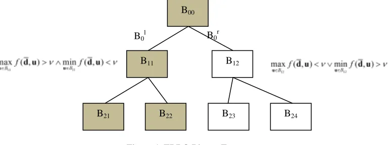
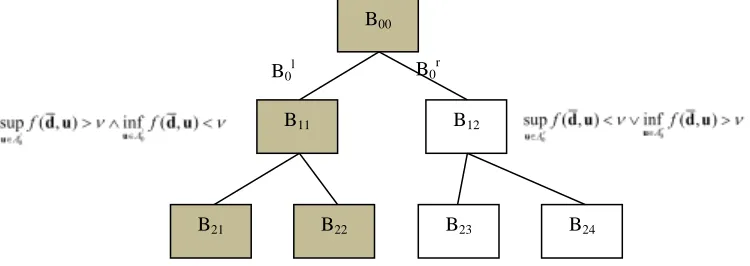
Given a design vector d, the value of Bel and Pl, for any value within [minmax], can be computed by building a binary tree in which a branch is pruned if the max of f associated to a leave is below (above) a given threshold . The binary tree is built as follows. The transformed uncertain space is partitioned by cutting every box
B
l i, (with0,0
B
U
) in two halves along the longest edge. The cutting point is the boundary of the uncertain interval that is the closest to the middle point of the edge. The tree is structured in levels with index l and at each level the tree has a number of leaves each one identified by the index i. Now letB
l il, andB
l ir, be respectively the left and right halves deriving from the partition of the i-th box (or leave)B
l i, at level l. If one box contains a maximum below the threshold or a minimum above the threshold the box is removed from the tree, otherwise it is added to the list of the boxes (leaves) that need to be partitioned at the following iteration (see Figure 1). If no maximum or minimum is yet computed either forB
l il, orB
l ir, then the box is added to the list of those that need to be explored. The boxes that need to be explored and partitioned are said to be undecidable as a decision cannot be made on whether they contribute to the Belief or not. The exploration of an undecidable box is performed by running a global maximization and a global minimization of f(d,u) for a fixed d and for l,l i
B
u
( r,l i
B
u
respectively). In this implementation, IDEA is used for both the global maximization and minimization. [image:6.612.125.512.330.474.2]
Figure 1. EBRO Binary Tree
Figure 1 shows a simple binary tree in which the right box deriving from splitting the initial uncertain space contains a maximum below the threshold or a minimum above the threshold. The whole branch of the tree is then discarded. The left box instead is undecidable and the branch that descends from that box needs to be explored. The branching and exploration proceed until a decision can be made for all the boxes. The exploration of a branch generates smaller and smaller boxes that eventually coincide with the focal elements. The exploration and branching process generates a number of focal elements clustered in macro boxes and a number of boxes that correspond to individual focal elements. All the discarded boxes with minimum above the threshold and all the boxes with maximum above the threshold are used to compute Pl(A). All the boxes with a minimum below the threshold are used to compute Pl A( ). The interesting aspect of this procedure is that Pl(A) and Pl A( ) can be computed even if all the maxima and minima are not identified exactly. In fact for a box to be included in the calculation of Pl(A)it is enough that a single value within the box, even not the actual maximum, is above the threshold. Likewise the calculation of Pl A( ) requires that even s single value, not necessary the actual minimum, is below the threshold.
Note that the collection of all the boxes generated for a given threshold can be used to compute the Belief (Plausibility) values in the interval [
max
]. In fact, the min and max values computed for each box represent additional values within [
max
]. However, while the value of Bel and Pl can be exactly computed for with the selected set of boxes, any other value within [
max
] might result to be an underestimation of Bel and overestimation of Pl because of a lack of resolution (i.e. each box includes an excessive number of focal elements).
B00
B11 B12
B21 B22 B23 B24
B0l B0
Therefore, if the whole curve is required, a refinement process is run by iteratively applying the evolutionary binary tree to the boxes that contain a given
max
[ ]
. This refinement process provides an exact value for each but can lead to a number of optimizations that is equal to two times the number of focal elements, if the entire curve is required. It is, however, interesting to note that if one takes an arbitrary max min
min
2
, the boxes generated
by the EBT can provide an approximation to the Bel and Pl curves that tend to be good in a neighborhood of
and close to max. This observation allows for the generation of a good estimation of the two curves at a fraction of the computational cost. Further to this approximation, two specific mechanisms have been devised to reduce the computational complexity and compute approximated Bel and Pl curves: the integrated focal element filtering and the approximated min and max evaluation.1. Integrated Focal Element filtering
The bpa associated to each focal element decreases in magnitude as the number of dimensions increases. This observation suggests that an approximation to the value of Bel and Pl can be computed by using only a selected subset of focal elements. The reduction in Bel or increase in Pl due to this approximation can be quantified by looking at the cumulative value of the discarded focal elements. Therefore, during the generation of the binary tree boxes with a bpa below a given filter threshold are discarded until the cumulative bpa associated to those boxes is below the required filter accuracy
2. Approximated Min and Max Evaluation
Because the calculation of Pl(A) and Pl A( ) does not always require the exam maximum and minimum, one can consider using an approximation of the min and max values for each subdomain Bl,i to make a decision. The evolutionary search for a maximum and a minimum proceed through an optimal sampling of the uncertain space. A selected subset of all the samples taken during the global exploration can be saved into an archive u
A, when maximizing, and into an archive into l
Awhen minimizing, Then when two new subdomains l, l i
B and r, l i
B are generated by bisection of Bl,i, one can take the maximum element sup
l
x in u l, l i
A B (respectively u r, l i
A B )and the minimum element infl
x in l l, l i
A B (respectively l r, l i
[image:7.612.129.504.437.570.2]A B ) instead of running a full optimization for every new box.
Figure 2. Binary Tree with Approximated Min-Max Evaluation.
Figure 2 shows a modified version of the binary tree in which decisions are made using the values in the archive instead of the actual maxima and minima. This technique produces a substantial reduction in the number of optimizations loops required to build the Belief and Plausibility curves but can introduce a significant error depending on the archiving procedure. In order to preserve accuracy the values
x
infl , suplx
,x
infr and suprx
are trusted to be representative of the minimum and maximum values contained in the box with a probability ptrust inversely proportional to the bpa associated to the box, i.e. the higher the bpa the lower the trust in the valuesx
infl andx
supl(respectively
x
infr and suprx
). In this way boxes with high bpa are properly explored with high probability. In B00B11 B12
B21 B22 B23 B24
particular, supl
x
and suprx
are trusted if ptrust>(c+bpa), where c is a trust factor. The use of a this trust factor ensure good accuracy for a single value of . During the refinement process, however, the EBT makes use of existing boxes but with different thresholds. Boxes that are correctly decided, on the basis of suboptimal archive values, for one threshold might not be correctly decided for a different threshold. When a new threshold is considered, the boxes generated for previous thresholds for which maximum and minimum was not exactly identified, are ranked from the one with highest bpa value to the one with the lowest. A maximization is then progressively run on each of them, starting from the one with highest bpa, until the cumulative bpa of the remaining ones is above c.IV TEST CASES
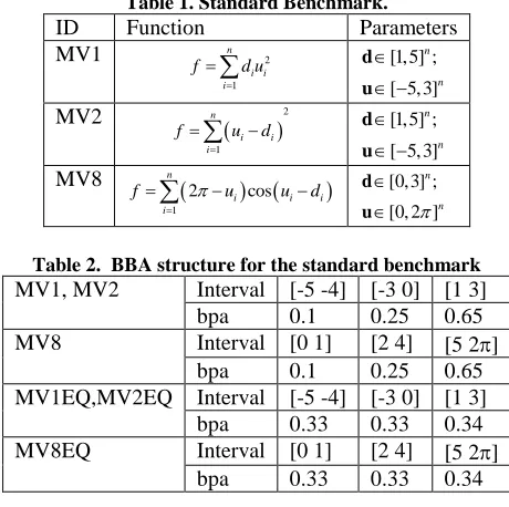
[image:8.612.190.420.296.525.2]The effectiveness of the techniques to reduce the computational cost has been put to the test on a set of simple but representative, scalable problems (see Table 1). All the problems present a number of maxima and minima that grows with the number of dimensions. Problem MV1 for example has a number of maxima in U that grows as 2n. Problem MV2 has maxima that change location with d while MV8 is multimodal and has the maxima that change with d. Table 2 represents the bpa structure for all the problems, with the intervals for each uncertain parameter and the associated bpa. Tests are run considering two possible different bpa structures: with a uniform distribution of bpa (labeled as EQ) and one with a non-uniform distribution. The tests in this paper are limited to three disconnected uncertain intervals per parameter but the results can be generalized to a higher number of intervals and also to overlapping intervals.
Table 1. Standard Benchmark.
ID Function Parameters
MV1 2
1
n i i i
f d u
[1,5] ;[ 5,3] n n d u
MV2 2
1
n i i i
f u d
[1,5] ;[ 5,3] n n d u
MV8
1
2 cos
n
i i i i
f u u d
[0,3] ;[0, 2 ]
n n d u
Table 2. BBA structure for the standard benchmark
MV1, MV2 Interval [-5 -4] [-3 0] [1 3]
bpa 0.1 0.25 0.65
MV8 Interval [0 1] [2 4] [5 2]
bpa 0.1 0.25 0.65
MV1EQ,MV2EQ Interval [-5 -4] [-3 0] [1 3] bpa 0.33 0.33 0.34 MV8EQ Interval [0 1] [2 4] [5 2]
bpa 0.33 0.33 0.34
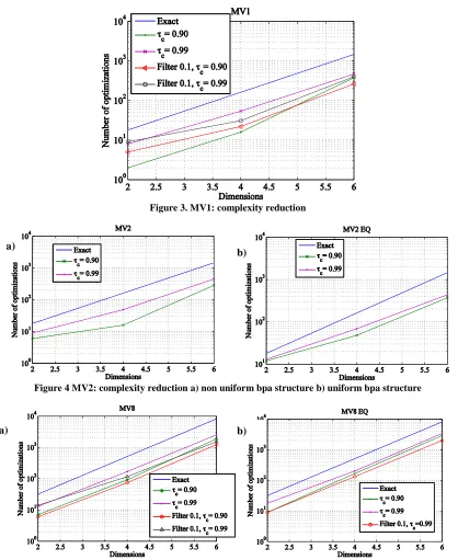
MV8. In this case the error in Belief for a trust factor of 0.90 is larger than 0.1 but for a very small difference in . The overall error in the decision of the reliability the estimation of a design margin would be contained but with a massive reduction in computational cost, up to 85%. It is also interesting to note that for all test cases the solution of the min/max problem returned the global maximum and an optimal d. IDEA was set with a population of 10 individuals for the inner loop and 500n/2 number of function evaluations. The population was restarted when the maximum distance among individuals was reaching 10% of the maximum distance experienced during the whole search. IDEA was set with a population of 10 individuals and 5000n/2 function evaluations. The population was restarted when the maximum distance among individuals was reaching 10% of the maximum distance experienced during the whole search, and the probability of running the global search in the inner loop was pd=0.5.
Figure 3. MV1: complexity reduction
[image:9.612.98.516.183.694.2]Figure 4 MV2: complexity reduction a) non uniform bpa structure b) uniform bpa structure
Figure 5 MV8: complexity reduction a) non uniform bpa structure b) uniform bpa structure
a) b)
a)
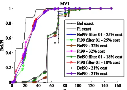
Figure 6 MV1: Bel and Pl curves at different approximation levels
Figure 7 MV8: Bel and Pl curves at different approximation levels
C. POWER-TELECOM INTEGRATED DESIGN PROBLEM
The techniques proposed in this paper were applied to the solution of a realistic case in which an integrated space system made of a power generation unit and telecom subsystem need to be designed under uncertainty. This section describes the power and telecom models used in this paper. The tests in this section aim to show how to use Evidence-Based Robust Optimization can provide a more precise quantification of the design margins, compared to a more traditional approach using rule of the thumb margins. The models in this section are derived from Ref. 16,17,18 and 19.
3. Power System Model
The power system (POW) model consists of a solar arrays and a battery. Starting from the required power in daylight and eclipse, the total required power is computed as:
e e d d
e d
sa
d
P T P T
+
X X
P =
T
(10)
where Pe is the power consumption during eclipse, Te is the orbital eclipse time, Xe is the energy transfer efficiency during eclipse, Pd is the power consumption during daylight, Td is the orbital daylight time, Xd is the energy transfer efficiency during daylight. The generated power at Beginning of Life (BOL)is:
o cell S
P =
G
(11)cos
BOL o d SA
P
= P I
(12)where Po is the ideal power output per unit area of the solar arrays, cell the solar cell efficiency, GS is the solar flux,
calculate the End of Life (EOL) power output per unit area, a solar array degradation over satellite lifetime factor Ld is calculated as follows:
1
Lifed cell
L =
(13)where cell is the array degradation per year, Life is the expected satellite lifetime. Once the satellite lifetime factor Ld is computed, the power output during EOL, PEOL, can be calculated, based on the power output per unit area PBOL, as follows:
EOL BOL d
P = P L (14)
Then the required solar array area Asa can be easily calculated as:
sa sa
EOL
P A =
P
(15) The solar array mass Msa is then derived from the solar array area Asa as follows:
sa sa sa
M = A
(16)where SA is the specific mass of the panel. The cell efficiency cell defines the type of solar cell that will be used including its intrinsic characteristics. For every value of cell a database of cells, see Table 3, is used to obtain the rest of the cell characteristics.
Table 3. Solar cell intrinsic characteristics.
CdTe p c-Si u c-Si 3j GaAs Conc. 3j GaAs
Multijunc. cells
ηcell 0.165 0.203 0.25 0.30 0.38 0.41
cell 1 0.037 0.037 0.05 0.05 0.05
The PCU power output Ppcu is calculated as follows: /
pcu sa pcu
P = P η (17)
where ηpcu is the PCU efficiency. Finally the PCU mass Mpcu is calculated as a fraction of the PCU power output:
pcu pcu pcu
M = a P (18)
where apcu is a PCU mass coefficient. The battery mass Mbat_pack, is computed starting from the energy density Ed, which defines the particular battery chemistry to be used (see Table 4). The efficiency depends on the type of battery and therefore on Ed. The efficiency ηbatt is computed by linearly interpolating the data in Table 4. Furthermore, using a simple linear relationship in logarithmic scale, the depth of discharge DOD is calculated as a function of parameter q in Table 4 and the number of cycles Ncycles. The number of cycles is derived from the orbital characteristics and a fixed input in this analysis.
Table 4. Battery intrinsic characteristics
NiCd NiH2 Ed (Wh/kg) 60 75
ηbatt (%) 85 86 q 145.8 176.3
The minimum required battery capacity Cmin can then be calculated as follows:
e e min
b
PT
C =
DOD
(19) and the mass of the battery cells Mb is calculated as:
min
b d C M =
E
4. Telecom System Model
The mass and power of the telecom system (TTC) are computed starting from the link budget. The required communication link characteristics are the Bit Error Rate BER, the modulation, and ground station antenna gain Gr. From the BER and modulation, one can compute the required energy per bit to noise ratio EbNo. The EbNo plus the data rate are used to compute the Carrier to Noise Ratio CNratio . The total amount of data to be transmitted is assumed to be 103
data
T = B where B is the total amount of data coming from the C&DH (Command & Data Handling) system to telecom. Given the access time ta the required data rate Rt is calculated as follows:
10
10 log data t
a aq
T R =
t – t
(21) where taq is the target acquisition time. Given the data rate and the bit to noise ratio, CNratio is simply:
0 ratio b t
CN E N R (22)
With the Carrier to Noise Ratio one can compute the Equivalent Isotropic Radiated Power (EIRP) as follows:
/
ratio TOTAL
EIRP
CN
G T
L
k
(23)where k = 228.6 dB, LTOTAL is the total signal loss and G/T is receiving system performance. The total signal loss is
computed adding up all the factors that lead to a loss of signal energy and an increase of the noise. Here most of these losses or sources of noise have been modeled with simple equations or look-up tables. The free space losses FSL are calculated from the distance from the ground station rGS as well as the frequency of the transmitter fT:
10 10
32.4
20 log
20 log
SL GS T
F
r
f
(24)The polarization mismatch (Ionospheric) losses PL can be computed from the Faraday rotation f using the following relationship:
10 20 log cos
L f
P = –
(25)The atmospheric losses AL are a function of the ground station altitude HG, are collected in a look-up table (as in Table 5) and interpolated. The dependency of the atmospheric losses on the elevation angle is modeled by introducing a simple sinusoidal function of the elevation angle e:
LH sin
L A
A =
e
[image:12.612.194.423.435.513.2](26)
Table 5. Atmospheric losses' change with ground station altitude
HG (km) AL (dB)
-2 to 2 0.04
2.1 to 6 0.025
6.1 to 10 0.008
10.1 to 14 0.004
14.1 to 18 0.001
The Rain absorption losses RaL are then calculated by using the data in Ref 16 and 18. The worst case losses for the Feeder loss FL, the Antenna misalignment loss AML and the implementation loss IL are reported in Table 6.
Table 6. Worst case losses
FL [dB] AML [dB] IL [dB]
2 0.5 2
Summing up all the individual losses provides the total loss LTOTAL:
TOTAL
FS
L LAM
L LH L aL LL
=
+ F +
+ A
+ P + R + I
(27) The system noise is computed from the antenna noise temperature ANtemp and from the cabling and receiver losses. The total noise gives the noise figure RNfig:
/10
/10
/10
/10
10 – 1 10 10 – 1
10
A A
AMP
L L F
o o
fig temp AMP G
k k
RN AN T (28)
where TAMP is the amplifier noise, LA the cable loss, GAMP the low noise amplifier gain, F the receiver noise figure
/10
/10
/10
10
– 1
10
10
– 1
/10
10
L L F
T T T
o o
temp tempT eT
GT
k
k
S
AT
T
(29)Here ATtempT is the transmitter antenna noise temperature, TeT is the transmitter amplifier noise, LT is the transmitter cable loss, GT is the transmitter low noise amplifier gain, FT is the transmitter noise figure. The rain noise Nrain is then calculated as follows:
rain /10
1
1–
10
RA oN
=
k
(30)where RA is the rain absorption. The total system noise TSnoise then writes:
10
10log
noise fig temp rain
TS
RN
S
N
(31)The receiving system performance G/T is then calculated as follows:
/
r–
noiseG T
G
TS
(32)where Gr is the ground station receiver gain. The required transmission power Pld onboard the spacecraft is defined as:
–
Ld t
P
EIRP
G
(33)where Gt is the transmitter antenna gain. The spacecraft antenna type is chosen on the basis of the required antenna gain Gt. It is well know that the best antenna for 5 dB ≤ gains ≤ 10 dB is the patch one, while the best for 10 dB < gains ≤ 20 dB belongs to the horn type set, therefore the mass of the antenna is computed as follows. The antenna characteristic length (it is the diameter of the normal conical section for conical horns, parabolas, and circular patches, and an equivalent diameter for pyramidal horns and square/rectangular patches) is:
0.5 10
10
t G ant ANT Tc
D
f
(34)where ANT is the antenna efficiency and c is the speed of light. If 5 ≤ Gt ≤ 10dB the mass of the patch is:
2
, 4
0.0015
0.0005
ant
D
ant patch diel copper
M
(35)where ρdiel = 2000 kg/m3 and ρcopper = 8940 kg/m3 are the averaged value of a dielectric material density and the copper density, respectively, considering a 2 mm total thickness, with 1.5 mm of dielectric material and 0.5 mm copper. If 10 dB < Gt ≤ 20 dB the lateral surface of the horn, SLAT, is computed as a conical surface:
2 2 2
4
ant D ant LAT hornD
S
L
(36)and the mass, Mant,horn, is:
,
ant horn LAT A
M
S
(37)where Lhorn is the length of the horn antenna can be assumed equal to 2Dant from available data, and ρA is the areal density, which has a mean value of approximately 15 kg/m2 (from available data18). If the gain of the antenna is > 20 dB, the parabola antenna is selected, the diameter of the antenna is computed with Eq.(34), and the mass of the antenna, Mant,par, is:
2
, 4
ant
D
ant par A
M
(38)where the surface density has a typical value of 10 kg/m2.
The mass of the amplifier Mamp is a function of PLd (see Ref. 17) as well as the mass of the case Mcase. An identification parameter T [0, 1] is used to identify the type of amplifier such that for TWTA type, T = 0 and for solid state type T = 1. Finally, the casing mass Mcase is computed as a fraction of the amplifier mass:
case amp CMR
M
= M
(39)5. Test Results
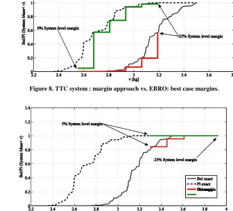
The bpa structure and the design space for both the TTC and POW system are summarized in Table 7 and Table 8. The assumption for the integrated system is that the power demand for the TTC, PLd, is added to a fixed power demand of 900W in daylight and 400W in eclipse. In these tests, it is assumed that the spacecraft spends half of the time in eclipse and half in daylight with a maximum solar aspect angle of 15degrees.
[image:14.612.132.481.290.648.2]Figure 8 and Figure 9 show the Bel and Pl curves for the TTC system and a comparison to the margin quantification using a traditional margin approach. The cost function f is the system mass, i.e. the mass of TTC. Note that some intervals are overlapping. This is an interesting feature of Evidence Theory that allows one to deal with what can be considered as the degree of ignorance on the bpa assignment. The assumption is that the spacecraft is operating at 1.5e6 km from the Earth and has an access time of 1000s to a ground station with a receiving antenna with a gain of 60dB. The volume of data is 120000 bits. The lifetime of the mission is assumed to be 4 years. The Faraday rotation is assumed to be 9 degrees, the gain of the ground station antenna 60dB and the BER is 1e-6. The ground station is assumed to be at altitude 0m with the spacecraft at 30 degrees of elevation angle. The gain of the amplifier is 60dB with cable losses of 8dB, a noise temperature of 400K, and a noise figure of 10. The transmitter amplifier gain is assumed to be 20dB with noise temperature of 400K and noise figure of 10. Note that the characteristics of the POW and TTC subsystems were not selected to reflect a real mission scenario but only to test the proposed methodology. With these values, the difference between the optimal and robust solution is about 1kg for the TTC.
Table 7. TTC bpa structure
ANT Interval [0.5 0.6] [0.65 0.75] [0.6 0.8] [0.8 0.95]
bpa 0.2 0.5 0.2 0.1
CMR Interval [0.1 0.2] [0.25 0.3] [0.1 0.3]
bpa 0.5 0.35 0.15
Lt Interval [1 2] [2 3] [3 5]
bpa 0.2 0.3 0.5
Tant
Interval [200 250] [300 370] [400 500]
bpa 0.1 0.6 0.3
Table 8. POW bpa structure
Xe Interval [0.5 0.6] [0.65 0.7] [0.72 0.75]
Bba 0.1 0.6 0.3
Xd Interval [0.65 0.7] [0.75 0.8] [0.8 0.85]
Bba 0.2 0.6 0.2
Id Interval [0.8 0.81] [0.82 0.83] [0.83 0.9]
Bba 0.7 0.2 0.1
PCU Interval [0.5 0.6] [0.65 0.7] [0.8 0.9]
Bba 0.1 0.6 0.3
Table 9. Design space for TTC and POW
Parameter Low bound Upper bound
fT (MHz) 7e3 11e3
Mod 0 1
T 0 1
Gt (dB) 5 20
cell 0.1 0.3
sa (kg/m2) 1 2
aPCU (kg/W) 0.01 0.02
Ed (Wh/kg) 60 100
A 25% margin is added to the mass of antenna and amplifier and then a system level margin is added as before to the total mass of the TTC. The two figures show that the margin approach either underestimates the Belief or overestimates the margin. Figure 8, in fact, shows that the Belief of the mass corresponding to the maximum system level margin is less than 60%. In the more conservative case, Figure 9, the Belief is 1 but the mass is overestimated by about 0.5kg.
[image:15.612.127.463.178.483.2]Figure 8. TTC system : margin approach vs. EBRO: best case margins.
Figure 9. TTC system: margin approach vs. EBRO: worst case margins.
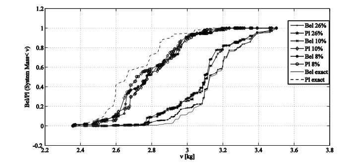
[image:15.612.134.456.326.489.2]Figure 10. Approximated Bel and Pl curves for the Telecom system
Figure 11 shows a similar result for the integrated Power and Telecom system. The total number of focal elements in this case is 8748 corresponding to 17496 optimizations for an exact calculation. The simple application of the integrated filtering technique beings a moderate reduction of computational effort down to 80% of the cost of the exact computation. The resulting Belief is underestimated by maximum 0.1. The application of the approximated min and max evaluation with c= 0.90 brings to a more substantial reduction, down to 22% and with a moderate overestimation that reduces almost to zero close to the left and right extremes of the Belief curve.
Figure 11. Approximated Bel and Pl curves for the integrated Power and Telecom system.
VI PROBLEM DECOMPOSITION
The interesting aspect of space engineering systems is that although the overall design requires the contribution of all the subsystems, some subsystems are relatively decoupled and exchange information only through their specific design budgets. For example, the telecom system and the power system exchange information only through the output power from the telecom system that becomes an input parameter to the power system.
Let us consider a function g D U: with the following form:
1 1 3 3 1 1 1 3
2
( ,
,...,
,
,
,...,
,
,
)
( ,
,...,
,
,...,
,
)
( ,
,
)
f
f f f f f
N
i i i N N N i i N N i i i i
i
g
f
f
d u
d u u
d
u
u
d u
d u
d
u
d u u
(40)Now assume that the functional dependency of function f1 on design and uncertain parameters di and ui is realized through a function hi such that:
1 1 3 3 1 1 1 3
2
( ,
,...,
,
,
,...,
,
,
)
( ,
,..., ( ,
),...,
(
,
))
( ( ,
),
)
f
f f f f f f
N
i i i N N N i i i N N N i i i i i
i
g
f
h
h
f h
If hi could be handled as independent variable the two functions f1 and fi could be decoupled and Bel(g<) could be expressed as:
1 1
1
1 1 1 3 3
( ) ( ) ( )
, |
, |
f
i i N
d i
A i A
i i i i
Bel g m m
A U U h g
A h U U g
u
u
(42)
If the value of the design parameters and of hi is fixed then the two functions are completely decoupled and the
computation of the Belief associated to their sum requires the independent computation of the maxima and minima of f1 and fi over the subspaces U1and U3i. If the range of hi is well defined then one could compute the values of fi for different values of hi by solving the following constrained problems:
3
3
max , ,
,
i
i i i
i i hi
f h
h
u d u
d u
(43)
If hi is fixed the computational complexity grows linearly Nf and the computation of the focal elements for each function fi can be performed in parallel. If the vector ui contains a single uncertain parameter the result is an exact representation of the Belief curve. If the vector ui contains multiple uncertain parameters then one can verify that the belief function Beld is equal to the full belief curve Bel only for the values for which the value of hi is verified. A good choice to fix the value of hi is to take the solution of the min-max problem (7). As an illustrative example consider the following toy problem:
2 2 2 2
2 1 2 21 22 32
21 22 2
1 3 1
1 2
2
f
d
d
u
u
u
h
u
u
f
d
u
h
g
f
f
(44)
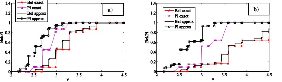
[image:17.612.87.535.534.665.2]Each uncertain parameter is defined over the three intervals [0 0.1], [0.2 0.4] and [0.5 1] with two different bpa assignments: a) 0.3, 0.6 and 0.1 respectively and b) 0.3, 0.1 and 0.6 respectively. Figure 12 shows a comparison between the exact Bel and Pl curves and the approximated ones. The approximated Bel curves are very close to the exact ones and are almost identical for some values of The Pl approximation is instead very poor for low values of and good for high values of The main reason is that only one value of h as used and it was the one corresponding to the solution of the min/max problem. All minimum values within the focal elements of the decomposed problem are therefore overestimated while the maxima are exact for a large number of focal elements at some specific . The main advantage of this approximation becomes clear when one looks at the computational cost. The exact computation requires 162 optimizations, while the approximated computation requires two parallel sets of optimizations with 3 optimizations per set, thus 6 in total. The computational cost of the approximation is therefore 3.7% of the cost of the exact computation and would grow linearly with the number of dimensions.
Figure 12. Decomposition approximation for bpa structure a) and bpa structure b)
VII FINAL REMARKS
The paper presented some strategies to obtain an estimation of Belief and Plausibility at a fraction of the computational cost for their exact calculation. The approach presented in this paper provides the computation of the optimal range of the design margin at a cost that is polynomial with the number of dimensions. An estimation of the full Belief and Plausibility corves could be obtained with a cost reduction by over 80% but maintaining a contained error. The effectiveness of the proposed strategies was proven on some benchmark problems, presenting a number of minima and maxima exponentially increasing with the number of dimensions. Furthermore, two space system design cases are used to show how evidence-based design optimization can improve the design of space systems compared to a more traditional system margin approach. From these test it appeared that, even in the ideal case in which an optimal deterministic design solution is available, a traditional margin approach tend to underestimate the reliability of the design margin or to overestimate their value, given the available information. This justifies the use of a rigorous margin quantification. Finally, a problem decomposition technique was proposed to reduce the computational complexity of space system design problems in which all the components contributing to the overall design budgets are only weakly coupled through a single function (the power in the case of space systems). For these particular problems, it seems possible to obtain massive reductions of the computational cost but, more importantly, a computational cost that increases linearly with the number of integrated systems. The results in this paper, however, are only preliminary and a more in depth investigation is underway.
Acknowledgments
This work is partially supported through an ESA/ITI grant AO/1-5679/08/NL/CB .
References
1
W. Oberkampf and J. C. Helton. Investigation of evidence theory for engineering applications. In 4th Non-Deterministic Approaches Forum, volume 1569. AIAA, April 2002.
2
H. Agarwal, J. E. Renaud, and E. L. Preston. Trust region managed reliability based design optimization using evidence theory. Collection of Technical Papers - AIAA/ASME/ASCE/AHS/ASC Structures, Structural Dynamics and Materials Conference, 5:3449 – 3463, 2003.
3
H.-R. Bae, R. V. Grandhi, and R. A. Canfield. Uncertainty quantification of structural response using evidence theory. Collection of Technical Papers -AIAA/ASME/ASCE/AHS/ASC Structures, Structural Dynamics and Materials Conference, pages 2135 – 2145, 2002.
4
T. Fetz, M. Oberguggenberger, and S. Pittschmann. Applications of plausibility and evidence thoery in civil engineering. In 1st International Symposium on Imprecise Probabilities and Their Appplications, Ghent, Belgium, 29 June- 2 July 1999.
5
L.-P. He and F.-Z. Qu. Possibility and evidence theory-based design optimization: an overview. Kybernetes. 6
Z. P. Mourela and J. Zho. A design 0ptimization method using evidence theory. Journal of Mechanical Design, 128:901 – 908, 2006.
7
T. Denoeux. Inner and outer approximation of belief structures using a hierarchical clustering approach. International Journal of Uncertainty, Fuzziness and Knowlege-Based Systems, 9(4):437 – 460, 2001.
8
J. C. Helton, J. Johnson, W. L. Oberkampf, and C. Sallaberry. Sensitivity analysis in conjunction with evidence theory representations of epistemic uncertainty.Reliability Engineering & System Safety, 91(10-11):1414 – 34, October 2006.
9
J. C. Helton, J. Johnson, W. L. Oberkampf, and C. Storlie. A sampling-based computational strategy for the representation of epistemic uncertainty in model predictions with evidence theory. Computer Methods in Applied Mechanics and Engineering, 196(37-40 SPEC ISS):3980 – 3998, August 2007.
10
J. C. Helton, J. Johnson, C. Sallaberry, and C. Storlie. Survey of sampling based methods for uncertainty and sensitivity analysis. Reliability Engineering & System Safety, 91(10-11):1175 – 209, October 2006.
11
M. Vasile. Robust mission design through evidence theory and multiagent collaborative search. Annals of the New York Academy of Sciences, 1065:152–173, Dec. 2005.
12
N. Croisard, M. Vasile, S. Kemble, and G. Radice. Preliminary space mission design under uncertainty. Acta Astronautica, 66:5 – 6, 2010.
13
G. Shafer. A Mathematical Theory of Evidence. Princeton University Press, 1976. 14
B. Tessem. Approximations for efficient computation in the theory of evidence. Artificial Intelligence. 15
M. Vasile, E. Minisci, and M. Locatelli. An inflationary differential evolution algorithm for space trajectory optimization. IEEE Transactions on Evolutionary Computation, 2011.
16
Dennis Roddy Satellite Communications 3rd ed., McGraw-Hill, 2001.
17 J. Larson, James R. Wertz Space Mission Analysis and Design 3rd ed. , Microcosm Press & Kluwer Academic Publishers.
18
Constantine A. Balanis Antenna Theory Analysis and Design 3rd ed. , Wiley-Interscience, 2005. 19

![Table 7. TTC bpa structure [0.65 0.75] 0.5](https://thumb-us.123doks.com/thumbv2/123dok_us/1679940.121394/14.612.132.481.290.648/table-ttc-bpa-structure.webp)