Quasi ALE finite element method for nonlinear water waves

      

City, University of London Institutional Repository

Citation

: Ma, Q. and Yan, S. (2006). Quasi ALE finite element method for nonlinear water

waves. Journal of Computational Physics, 212(1), pp. 52-72. doi: 10.1016/j.jcp.2005.06.014

This is the accepted version of the paper.

This version of the publication may differ from the final published

version.

Permanent repository link:

http://openaccess.city.ac.uk/4324/

Link to published version

: http://dx.doi.org/10.1016/j.jcp.2005.06.014

Copyright and reuse:

City Research Online aims to make research

outputs of City, University of London available to a wider audience.

Copyright and Moral Rights remain with the author(s) and/or copyright

holders. URLs from City Research Online may be freely distributed and

linked to.

Editorial Manager(tm) for Journal of Computational Physics Manuscript Draft

Manuscript Number: JCOMP-D-05-00185R1

Title: Quasi ALE finite element method for nonlinear water waves

Article Type: Regular Article

Section/Category:

Keywords: QALE-FEM; Nonlinear water waves; Spring analogy; Periodic bars; Free surface.

Corresponding Author: Dr Qingwei Ma, PhD

Corresponding Author's Institution: City University

First Author: Qingwei Ma, PhD

Order of Authors: Qingwei Ma, PhD; S. Yan

Quasi ALE finite element method for nonlinear water waves

Q.W. Ma and S. Yan

School of Engineering and Mathematical Sciences, City University, Northampton Square, London, EC1V 0HB UK

Abstract

This paper presents a newly developed quasi arbitrary Lagrangian-Eulerian finite element method (QALE-FEM) for simulating water waves based on fully nonlinear potential theory. The main difference of this method from the conventional finite element method developed by one of authors of this paper and others (see, e.g., [11] and [22]) is that the complex mesh is generated only once at the beginning and is moved at all other time steps in order to conform to the motion of the free surface and structures. This feature allows one to use an unstructured mesh with any degree of complexity without the need of regenerating it every time step, which is generally inevitable and very costly. Due to this feature, the QALE-FEM has high potential in enhancing computational efficiency when applied to problems associated with the complex interaction between large steep waves and structures since the use of an unstructured mesh in such a case is likely to be necessary. To achieve overall high efficiency, the numerical techniques involved in the QALE-FEM are developed, including the method to move interior nodes, technique to re-distribute the nodes on the free surface, scheme to calculate velocities and so on. The model is validated by water waves generated by a wavemaker in a tank and the interaction between water waves and periodic bars on the bed of tank. Satisfactory agreement is achieved with analytical solutions, experimental data and numerical results from other methods.

Keywords: QALE-FEM; Nonlinear water waves; Spring analogy; Periodic bars; Free surface.

1. INTRODUCTION

With operations in the oil and gas industry moving to deeper waters, offshore structures are more likely to be exposed to very harsh environments and extremely steep waves and therefore undergo large motions. As a result, there is increasing interest in numerically simulating nonlinear water waves and their interaction with structures. There are two classes of theoretical models for cases with finite water depth in common use for numerical simulations. One is based on the general flow theory and the other is based on the potential theory. In the first class of models, the Navier-Stokes and continuity equations together with proper boundary conditions are solved, while in the second class, the Laplace equation with fully nonlinear boundary conditions is dealt with. For brevity, the first class of models will be called NS Model and the second called FNPT (representing fully nonlinear potential theory) Model in the paper.

In the community of researchers who use the NS Model, three formulations have been suggested: Eulerian, Lagrangian and arbitrary Lagrangian-Eulerian (ALE) formulations. In the Eulerian

formulation, the computational mesh is fixed and the fluid moves relative to it (see, for example, [1] – [4]). Use of this formulation can handle, with relative ease, the large distortions of interfaces between two different materials by employing proper interface capturing techniques (such as volume of fluids, level set method and so forth) but possibly at the expense of solving a larger domain than necessary, solving an extra governing equation and smearing the interfaces and flow details near the interfaces. In addition, it seems to be difficult to handle cases with interfaces of three different materials, such as those with floating bodies in waves. In the Lagrangian formulation (see, for instance, [5]), all nodes follow their corresponding fluid particles. Due to this feature, the formulation allows sharp tracking of interfaces between different materials. However, if large distortions of the fluid domain occur, certain nodes may become too close to or too far from others and consequently lead to a breakdown of the computing process if remeshing is not performed. The arbitrary Lagrangian Eulerian (ALE) formulation is a hybrid approach, in which the computational mesh does not need to adhere to fluid particles or to be fixed in space but can be moved arbitrarily. Therefore, the ALE formulation can make use of the merits of both the Lagrangian and Eulerian formulations and alleviate many of their drawbacks. Specifically, the interface can be precisely tracked without necessarily remeshing. Of course, the nodes have to be moved in order to conform to the deformation or distortion of interfaces or boundaries and the governing equations are made a bit more complex to account for the moving velocities of mesh. The ALE formulation has been discussed and used in many publications. Only a few are listed here as examples [6] – [8]. Various numerical methods, such as finite element, finite volume and finite different methods have been used to solve the Navier-Stokes and continuity equations together with one of three formulations to investigate the nonlinear water waves and their interaction with fixed structures. However, no matter which method is used, solving NS equations is always a time consuming task.

procedure, the key task is to solve the boundary value problem by using an efficient numerical method. To do so, boundary element methods (BEMs) have been used in many publications, such as [10] and [14]-[17], and have produced many impressive and useful results. Finite element methods (FEMs) have also been developed and used for two and three dimensional problems, see, for instance [11]-[12] and [18]-[24]. Both methods have been proved quite efficient but the FEMs need less memory and so are computationally more efficient, as indicated by Wu & Eatock Taylor [19] and Ma, Wu & Eatock Taylor [11]. The reason is that although there are far fewer unknowns when using the BEMs than using the FEMs, nonzero elements in the matrix for the BEMs may be more than those in the matrix for the FEMs since any node in the BEMs is affected by all others, while in the FEMs only by those connected with the node. A drawback of the FEMs, however, is that an unstructured mesh is generally required for complex interaction between water waves and structures and may need to be remeshed at every time step to follow the motion of waves and/or structures. Repeatedly regenerating such a mesh can make the required CPU time prohibitive in a simulation of several thousands steps on a normal workstation. In order to reduce the time spent on the remeshing, simple structured mesh has been used in [11] and [12]. For the same purpose, Wu et al. [22] have recently employed a hybrid mesh. In their approach, a 2D mesh in a horizontal plane (say, the free surface at t=0) is first generated and then vertical lines are drawn to construct a 3D mesh. The 2D mesh is formed by combining an unstructured mesh in a region near structures with a simple structured mesh (similar to [23]) in other regions. This is a sensible approach but restricted to cylindrical structures without roll and pitch motions.

mesh. An efficient and accurate technique will also be suggested for the velocity computation in this paper.

Although the QALE-FEM based on the FNPT Model can be used to deal with any wave/structure interaction problem without wave overturning/breaking, this paper focuses on the description of the method and validates for cases without floating bodies. Applications to more general cases will be given in other papers.

2. MATHEMATICAL MODEL AND NUMERICAL METHOD

Without loss of generality, the computational domain is chosen as a rectangular tank, and the nonlinear wave is generated in the tank by a piston-like wavemaker. The wavemaker is mounted at the left end (on the negative side of the x-axis) and a damping zone with a Sommerfeld condition (see [11] and [12] for details) is applied at the right end of the tank in order to suppress the reflection, as sketched in Fig. 1. Arbitrary forms of submerged bodies on the tank-bed may be included. A Cartesian coordinate system is used with the oxy plane on the mean free surface and with the z-axis being positive upwards. Unless mentioned otherwise, its origin will be located at the centre of the tank.

[image:6.595.127.460.369.530.2]

Wavemaker Damping zone

Fig. 1 Sketch of fluid domain

Similar to the usual formulation for the FNPT Model, the velocity potential (

φ

) satisfies Laplace’s equation

0

2

₌

∇

φ

(1)

in fluid domain. On the free surface z=ς

(

x,y,t

)

, the velocity potential satisfies the kinematic and dynamic conditions:

z

dt

Dz

y

dt

Dy

x

dt

Dx

∂

∂

=

∂

∂

=

∂

∂

=

φ

,

φ

,

φ

(2)

2

2

1

_φ

φ

∇

+

−

=

gz

Dt

D

(3) in which g is the gravitational acceleration. The atmospheric pressure has been taken as zero in Eq.

d

B

L

Lm b

y

x z

(3). On all rigid boundaries, the velocity potential must satisfy

)

(

t

U

n

n

r

r

_⋅

=

∂

∂

φ

(4) where

U

r

( )

t

and is the velocity and the unit normal vector of the rigid boundaries, respectively. For

the specific case illustrated in Fig. 1,

nr

( )

t U

( )

t

Ur = _x on the wavemaker and

U

r

( )

t

=

0

on other rigid boundaries.

The problem described by Eqs. (1) to (4) will be solved by using a time step marching procedure as outlined in the Introduction. At each time step, the shape of the free surface and the potential values on it as well as velocities on all rigid boundaries are known (given as initial conditions or calculated from the solution at previous time steps). Thus, at an instant, the boundary condition for the potential on the free surface can be replaced by a Dirichlet condition:

p

f

=

φ

, (5)

where is the potential values on the free surface at the instant. Therefore, the unknown velocity potential in the fluid domain can be found by solving a mixed boundary value problem which is defined by Eqs. (1), (4) and (5). After the solution is obtained, Eqs. (2) and (3) are then employed to update the position of and the potential values on the free surface using the same method as in [11], which gives the new information on the free surface for the solution at next time step. If floating bodies are included, the dynamic governing equations of the bodies should be solved at this point to update the velocity in Eq. (4). Similar to [11], the finite element method is used to solve the mixed boundary problems, in which the fluid domain is discretised into a set of small tetrahedral elements and the velocity potential is expressed in terms of a shape function,

p

f

(

)

N x y z

_J

, ,

:

∑

=

J

J

J

N

(

x

,

y

,

z

)

φ

φ

(6)

where φ_Jis the velocity potential at node J. Using the Galerkin method, Laplace’s equation with corresponding boundary conditions can be discretised as

∫∫∫

∑

∫∫

∫∫∫

∑

∀ ∉ ∀ ∈

∀

∇

⋅

∇

−

=

∀

∇

⋅

∇

P _n P

S

J J S

J J p I S n I J J

I

N

d

N

f

dS

N

f

N

d

N

φ

(

)

(

I∉S_P

)

(7)

where

S

P

represents the Dirichlet boundary (such as the free surface), on which the velocity

potential

f

p

is known and

S

n

represents the Neumann boundary (such as the wavemaker), on

[ ]

A

{ } { }

φ

= B (8) where

{ }

[

₁, ₂, ₃, , ,

]

T ( _P)

I I∉S

=

φ

φ

φ

_K

φ

_K

φ

(9)

(

P P

J I

IJ N N d I S J S

A =

∫∫∫

∇ ⋅∇ ∀ ∉ ∉

∀

,

)

(10)

(

P

)

S J

J J p I

S n I

I

N

f

dS

N

f

N

d

I

S

B

P n

∉

∀

∇

⋅

∇

−

=

∫∫

∫∫∫

∑

∀ ∈

)

(

(11)

The algebraic Eq. (8) is solved using a conjugate gradient iterative method with SSOR preconditioner and optimised parameters. Details about these have been discussed by Ma [24].

3. MESH MOVING IN QALE-FEM

As indicated in the Introduction, the main task in the QALE-FEM is to move the mesh so as to accommodate large variations in the fluid domain. In order to achieve high efficiency and accuracy of the computation, the method to move the mesh should satisfy the following criteria:

• It must create satisfactory element shapes at all time steps.

• It must preserve reasonable refinement and distribution in regions of interest, such as those close to the free surface and structures.

• It must be computationally efficient.

Many methods to move the mesh in the ALE formulation have been suggested for the NS Model. Often-used methods include the weighted average method [25], the transfinite mapping method [26], the method based on the solution of a linear elastic equation to define the new positions of nodes [8], the method based on the solution of Laplace’s equation to find the velocity of mesh [27] and so forth. These methods either tend to make the mesh uniform, need a special mesh structure or require much computational time and so they are not perfect options satisfying the above criteria.

In order to achieve a reasonable quality of the mesh at all time steps and avoid excessive computational time spent on moving the mesh, the following strategies are adopted to move the mesh in this paper:

• ensuring that there are no nearly flat elements in the initial mesh; • considering interior nodes and boundary nodes separately;

• considering nodes on the free surface and on rigid boundaries separately;

• using relatively stiffer springs near the moving boundaries, such as the free surface. The quality of initial mesh is to be achieved using mesh generators based on available technologies, such as mixed Delaunay triangulation and the advancing front technique [33]. The interior nodes are moved by using the linear spring analogy method. This method has been developed in computational aerodynamics, see e.g. [28], as indicated above. For completeness, it is only briefly described here. More details can be found in the references given. In this method, the nodal displacement are determined by

∑

∑

= =

∆

=

∆

i Ni

j ij N

j

j ij

i

k

r

k

r

1 1

r

r

₍₁₂₎

where is the displacement at Node I; kijis the spring stiffness and Niis the number of nodes that

are connected with Node I. Eq. (12) can be interpreted as that the resultant spring forces acting on Node I by all springs remain zero after all nodes are displaced. The value of the spring stiffness in the equation is usually chosen to be inversely proportional to the distance between two nodes in other applications [28] [30]. For the applications concerned with in this paper, it is found that the spring stiffness is best taken to be

i

r

r

∆

( ) [ z z d ij

ij _l e i j

k = 1₂ γ1+ + 2 ] (13)

where lij is the distance between Nodes I and J; zi and zj are the vertical coordinates of Nodes I and J; d

is the water depth; and γ is an coefficient that should be assigned a larger value if the springs are required to be stiffer at the free surface. The value of γ is taken as 1.7 in this paper but further numerical tests may be needed to choose the value of γ based on the wave steepness. To solve Eq. (12) for all interior nodes, iteration is required at each time step but it takes only a little CPU time according to our experience. The nodes at all rigid boundaries are also moved using the spring method.

3.1 Moving the nodes on the free surface

nodes are relocated at some time steps (e.g., every 40 time steps). For the purpose of relocation, they are grouped into those on curved waterlines, such as the intersecting line between the free surface and vertical walls or the wavemaker, and those that do not lie on the waterlines. The nodes in the latter group are called inner-free-surface nodes.

The nodes in the two groups are treated separately. The nodes on the waterlines will be re-distributed by adopting a principle for self-adaptive mesh, see [34] for an example. The basic idea is to make the weighted arc-segment lengths between two successive nodes a constant along the curved waterlines, i.e.

s i i

∆

s

=

C

ϖ

(14)

where

ϖ

is a weighted function, the arc-segment length between two successive nodes and Cs a

constant. The value of Cs is determined by using the fact that the total length of the curved waterline

(Ls), should equal the sum of all arc-segment lengths, which gives i

s

∆

s s i s

s

L

L

C

χ

ϖ

=

=

∑

1

(15)

where

=

∑

i

s

_ϖ

χ

1

. Therefore, if the weighted function is given, the arc-segment lengths can be evaluated by s i s i

L

s

χ

ϖ

=

∆

. (16)

The distribution of is controlled by the weighted function. An arc-segment tends to be smaller for a larger value of the weighted function or vice versa. In [34], the weight function is specified as

i

s

∆

β

α

ϖ

=

1

+

~

f

(17)

where αand β are two coefficients and

~

f

is the function of the gradient of a variable, such as velocity. For the applications considered in this paper, is taken as a function of the curvature of the curved waterline, i.e., it is given by

f

~

(

) (

)

[

_κ

_κ

_κ

_κ

β

α

ϖ

_i =1+ _i − _{min max} − _min

]

(18)

where

κ

_i is the curvature of the curve

∆

s

_i ;

κ

_max and

κ

_min are the maximum and minimum curvatures of the waterline, respectively. It is suggested in [34] that the coefficient α is determined by the arbitrarily-specified maximum (

∆

s

_smax) and minimum (

∆

s

_smin ) length of the arc-segment elements, i.e.

1

min max

₋

∆

∆

=

s s

s

s

α

. (19)

is larger in areas of longer waves. Hence it is reasonable to specify min max min max

L

L

s

s

s s

₌

∆

∆

(20)

where Lmax and Lmin are the maximum and minimum wave lengths, repetitively, which can be roughly

estimated for problems considered. It should be noted that α subjected to Eq. (20) becomes zero for waves with single wavelength and so the arc-segment lengths are a constant after the nodes are re-distributed. Such a distribution of nodes is reasonable for these cases. The evaluation of β is not so straightforward. In [34], this value is determined in such a way that the minimum length of arc-segment elements obtained by Eq. (16) is approximately equal to the specified ∆ssmin. To achieve this,

iteration must be performed. According to our numerical tests, a value of β in the range of 0.5 ~1.0 can lead to a satisfactory distribution of

∆

s

_iwhen Lmax/Lmin<10.

Once the nodes on the waterlines are redistributed, the inner-free-surface nodes will be moved by the spring analogy method, as used for the interior nodes. Nevertheless, there exists a difficulty, that is, how to ensure the nodes after moved are still on the free surface represented by discrete points. For simplicity, a method to achieve this is that the nodes are first moved in the projected plane of the free surface, i.e., calculating the values of x and y of new nodes using the spring analogy system, and then the elevations of the free surface corresponding to them are evaluated by an interpolating method. In order to take into account of the local gradient of the free surface, the spring stiffness in moving the nodes in x- and y- directions, however, is determined respectively by:

( ) 2

2 1 1 ⎟ ⎠ ⎞ ⎜ ⎝ ⎛ ∂ ∂ + = x l k ij x ij ς

and ( )

2 2 1 1 ⎟⎟ ⎠ ⎞ ⎜⎜ ⎝ ⎛ ∂ ∂ + = y l k ij y ij ς . (21) where x ∂ ∂ς and y ∂ ∂ς

are the local slopes of the free surface in the x- and y-directions, respectively. Inclusion

of free-surface slopes in the spring stiffness ensures that the spring forces acting on a node are proportional to relative displacements between nodes measured along the curved free surface rather than along horizontal directions.

the technique for moving the inner-free-surface nodes described here may not work if overturning/breaking waves are involved, which are beyond our consideration based on the FNPT Model.

4. VELOCITY CALCULATION ON THE FREE SURFACE IN QALE-FEM

It is crucial in simulating water waves to evaluate the fluid velocities on the free surface because they are used to update the information on the surface every time step. The velocity at a node may be estimated by using a finite difference technique from the velocity potentials at this node and nodes connected to it. The approach is quite efficient. However, since the neighbours of a node on the free surface are distributed either on or below the surface, the normal (or nearly vertical) component of the velocity estimated by the approach generally possesses relatively low accuracy, which is understandable from the fact that backward or forward finite difference schemes approximating a derivative have a lower order of accuracy than a central scheme. In order to enhance the overall accuracy, Ma, Wu & Eatock Taylor [11] suggested that the horizontal components of the velocities at nodes on the free surface are evaluated separately from their vertical components. For estimating the vertical component, they developed a three-point formula that needs the velocity potentials at the node considered and at two other nodes on the same vertical line as this node, which are next but just below the free surface. After the vertical component is found, the horizontal components are computed by averaging those given by the difference of the velocity potentials at all neighbour nodes on the free surface. This approach is very efficient and accurate. However, it is limited to structural meshes with vertical grid lines.

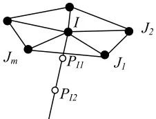
In this section, the above approach will be extended to unstructured meshes generally without vertical grid lines. The basic idea of the new approach is similar to the above approach. The main differences are that (1) the vertical line is replaced by a normal line perpendicular to the free surface at the node considered; (2) the two nodes on the vertical line are replaced by two points on the normal line, which do not necessarily coincide with any nodes; and (3) the normal component of the velocity is found before computing the components in tangential directions. More details are given below.

I _J

2

Jm P_{I1 J1}

[image:12.595.240.353.591.677.2]

PI2

Fig. 5 Sketch of nodes around Node I

Consider Node I on the free surface of an unstructured mesh with nodes Jk(k=1, 2, 3, . . . , m) as

points PI1 and PI2 are chosen on this line, as shown in Fig. 5. The distance between I and PI1 is hI1 and

the distance between PI1 and PI2 is hI2. The normal component (

v

r

_n) of the velocity at Node I is

calculated by n h h h h h h h h h h h v I I P I I I I P I I I I I I I I n r r ⎥ ⎦ ⎤ ⎢ ⎣ ⎡ ⎟⎟ ⎠ ⎞ ⎜⎜ ⎝ ⎛ + + ⎟⎟ ⎠ ⎞ ⎜⎜ ⎝ ⎛ + − ⎟⎟ ⎠ ⎞ ⎜⎜ ⎝ ⎛ + + + = 2 1 2 1 1 2 1 2 2 1 2 1 1 3 2 1 3 2 2 1 2 3

2 _{φ φ φ}

. (22) where is the unit normal vector of the free surface at Node I. This equation is similar to Eq. (16) in

[11]. Nevertheless,

nr 1 I P

φ

and 1 I P

φ

here are not nodal values and may be found using the method discussed in subsection 4.1 below. The normal vector is taken as the average of the normal vectors of all surface elements (such as I-J1-J2 ) with Node I as one of their nodes.

In order to estimate the velocity in tangential directions, the unit tangential vector (

τ

r) is required. The vector may be determined by using

τ

r

_x

⊥

n

r

,

τ

r

_x

//

e

r

_x,

τ

r

_y

⊥

n

r

and

τ

r

_y

//

e

r

_y, where and

e

r

_x

e

r

_y are the unit vectors in the x- and y-directions, respectively. The tangential components of the velocity are related to the difference of the velocity potential between any pair of nodes containing Node I and one of Nodes J1, J2,. . . , Jm by

k k

k y k

x

l

IJ

v

l

IJ

l

IJ

v

n

l

IJ

v

r

_τ

⋅

r

+

r

_τ

⋅

r

=

r

⋅

∇

φ

−

r

⋅

r

( k=1, 2, 3, . . . , m) (23) where

k

IJ

l

r

is the unit vector from Node I to Node Jk;

v

r

τ_x and vτy

r _{represent the velocity components in}

x

τ

r

and

τ

r

_y directions, respectively. The number (m) of equations in Eq. (23) is usually larger than 2, the number of unknowns. In order to use all the equations and enhance the accuracy, the least square method is adopted to find

x

v

r

_τ and . Once the three components are obtained, the velocity components in x-, y- and z-directions can readily be computed by projecting them on these directions.

y

vr_τ

4.1 Velocity potential at Points PI1 and PI2

There are two issues associated with the velocity potential at Points PI1 and PI2,involved in the

above velocity computations. One is how to choose the positions of the points and the other is how to estimate the values of the potential at these points. According to our experience, Point PI1 should be

located in the element connected to Node I and Point PI2 should be in another element next to the

previous element in the normal direction. This is rational from simple reasoning. If the two points are too close to Node I so that they fall into one element, the values of potential calculated at these points are based mainly on the information of one element and so the estimated difference by using these values may possess low accuracy. On the other hand, if the points are too far from each other or from Node I, the error of velocity estimated using Eq. (22) may also be big because the error increases with distances between them.

In order to ensure the two points to be in the desired elements, hI1 and hI2in Eq. (22) can be determined

h

ε

= = ₂

1 I

I h

h , (24)

where

ε

is the coefficient and

_h

is the distance from Node I to the intersecting point of the normal line I-PI1-PI2 with the element surface formed by other three interior nodes of the element connected to

Node I. Numerical tests show that ε may be a value in the range of 0.6 ~ 0.9 and that numerical results obtained are not sensitive to its specific value. The numerical tests also show that the value of does not necessarily have to be calculated every time step. In fact, it is calculated only at the first time step for cases presented in Section 5.

h

With the values of hI1 and hI2determined, the values of the potential at Points PI1 and PI2 can be

estimated either by using the shape function defined on the elements or by the MLS method mentioned above. The former method needs less computational time but gives less accurate values, particularly in cases with large gradients. The latter requires more computational time but results in more accurate potential values. If the waves to be simulated are very steep, the latter should be used; otherwise the former would be the better choice. Because we aim at steep waves, the latter is used in this paper.

4.2 Special treatment for nodes near solid boundaries

It may become impractical to use the above method to calculate the velocity for nodes near a solid boundary because the normal line I-PI1-PI2 may intersect with the solid boundary (see Fig. 6). If this

happens, either Point PI2 is put outside the fluid domain if hI1and hI2 are still estimated by Eq. (24) or

the two points (PI1 and PI2) are contracted into one element. Both situations may degrade the results.

nr b

n

r

b

τ

r

Solid boundary

Free surface Fig. 6 Nodes near a solid boundary

In order to avoid such problems, it is proposed that the normal line (coinciding with vector nr in Fig. 6) at a node near a solid boundary is replaced by a line (coinciding with vector

n

r

_b) obtained by rotating the normal line to the direction perpendicular to the normal vector, passing the node considered, of the boundary surface. Correspondingly,

τ

ris replaced by

τ

r

_bthat is determined by

n

r

_b,

x

e

r

and

e

r

_y using the similar method to that for

τ

r. After doing so, Eqs. (22) and (23), by substituting

b

when the wave tends to overturning, which is not considered in this paper, as indicated above.

5. NUMERICAL VALIDATIONS

In this section, the QALE-FEM method is validated by comparing its numerical predictions with analytical solutions and published results using other methods or experiments. Two kinds of problems are considered: one is nonlinear water waves (regular and random) generated by a wavemaker in a tank; and the other is the interaction between the water waves and periodic bars on the tank-bed. For all the cases in this section, the maximum and minimum wave lengths in Eq. (20) are assumed to be the same. In the following, all parameters with a length scale are nondimensionalised by the water depth d and other parameters by

g d

t→τ / and ω→ω g/d .

5.1 Water waves generated by a wavemaker

[image:15.595.100.503.532.725.2]

Water waves generated by a piston wavemaker in the tank are considered in the first instance. The waves may be monochromatic, bichromatic and random depending on the motion of the wavemaker. The meshes used are similar to that in Fig. 7 but much finer.

Fig. 7 Illustration of initial mesh used for wavemaker problems

-2.0 0.0 2.0

-7 -5 -3 -1 x 1 3 5 7

ς/a

(a) (a) τ = 10T

-2.0 0.0 2.0

-7 -5 -3 -1 x 1 3 5 7

ς/a

(b) τ = 15T

The cases of monochromatic waves are first modelled, for which the motion of the wavemaker is governed by

( )

τ acos

( )

ωτ

S =− , (25a)

( )

τ aωsin

( )

ωτ

U = , (25b)

where S

( )

τ is the displacement of the wavemaker, U

( )

τ is its velocity, a and ω are respectively its amplitude and frequency. When the amplitude of the wavemaker is very small, the steepness of the generated waves is also very small. The numerical results for such a case can be compared with the linearised analytical solution in [42]. For this purpose, a case with a =0.0041 and ω=1.45 is simulated in a tank of length L ≈ 14.7. The mesh is unstructured and the number of elements is about 78060. The time step is 0.021666, about 200 steps in each period. The wave profiles at two different instants (t=10T and 15T, where T =2π/ω is the period) are plotted in Fig. 8, which shows that the numerical results are in very good agreement with the corresponding analytical solution.

The numerical results in Fig. 8 are also assessed by estimating relative errors. The relative error (Er) is defined as:

a a r

E ς

ς ς − =

where =

∫

e

A

dA

2

ς

ς , ς_a is an analytical wave elevation and Ae is the area over which the error is

estimated. Because the accuracy of the waves within the damping zone should not be of concern, Ae

equals the area of the free surface minus the part of the damping zone. The relative errors evaluated in this way for the results in Fig. 8 are less than 0.5%.

-2.0 0.0 2.0

-7 -5 -3 -1 x 1 3 5 7

ς/a

(a) τ = 10T

-2.0 0.0 2.0

-7 -5 -3 -1 x 1 3 5 7

ς/a

[image:16.595.94.508.505.700.2]

(b) τ = 15T

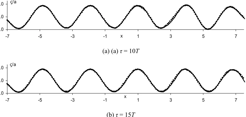
Fig. 9 Comparison of wave profiles for ω=1.45 and a=0.082 (Solid line: QALE-FEM; Dots: conventional FEM [11])

and strong nonlinearity. The amplitude of the wavemaker is taken as 0.082. The frequency (ω) and tank length are the same as that in Fig. 8. The steepness of the generated waves is about 0.08. For such steep waves, the linearised solution should not be considered valid. In order to validate the QALE-FEM in this case, its results are compared with those obtained by using conventional FEM described in [11]. The length of the time step (also 200 steps in each period) is the same in both methods, whereas the type of mesh and the number of elements are different. When using the conventional FEM [11], the mesh is structured and the number of elements is 75264. When using the QALE-FEM, the mesh is unstructured and the number of elements is about 78060. The latter is also tested using a larger number of elements (133632) but no significant difference in results was found. The wave profiles at time τ = 10T and 15T from these two methods are depicted in Fig. 9. The agreement between them is quite good. The relative error estimated by the same method for Fig. 8 is found to be less then 1%.

The QALE-FEM has also been used to simulate bichromatic waves. These waves are generated by the following motion of the wavemaker

( )

τ a₁cos

( )

ω₁τ a₂cos

( )

ω₂τ

S =− − (26a)

( )

τ a₁ω₁sin

( )

ω₁τ a₂ω₂sin

( )

ω₂τ

U = + (26b)

where a1 and a2 are the amplitudes corresponding to the components with frequencies ω1 and ω2,

respectively. As an example, the values for these parameters are assigned as a1=0.016, a2=0.5a1,

ω1=1.45 and ω2= 2.03. The tank has the same length and the mesh is the same as for Fig. 9. The time

step is about 0.01548, about 200 steps in each period given by 2π/ω2. For this case, the wave history

recorded at a fixed point is plotted in Fig. 10, together with the results from the conventional FEM. Again, it is observed that results from the two methods are in very good agreement and the relative error is in the same level as for Fig. 9.

-3.0 -1.5 0.0 1.5 3.0

10 20 30 40 τ 50 60 70 80

[image:17.595.81.514.529.617.2]

ζ /a1

Fig. 10 Comparison of wave histories for a1=0.016, a2=0.5a1, ω1=1.45 and ω2= 2.03

-0.2 -0.1 0 0.1 0.2

40 50 60 τ

ς

Measured

Numerical

-0.2 -0.1 0 0.1 0.2

40 50 60 τ

ς

Measured

Numerical

[image:18.595.107.491.80.218.2]

(a) (αrandom = 0.612) (b) (αrandom = 0.749)

Fig. 11 Comparison of wave histories at x =3.436 with measured data given by Nestegard [43]

As another example, the QALE-FEM is applied to simulating random waves. In order to compare with the experimental results given by Nestegard [43], the same motion of the wavemaker as those described in [43] is used, which is specified by a Fourier series with different scaling factors (αrandom).

The water waves generated by this motion are focused at a point in the tank to form a large and steep wave. To model this case, the tank length is chosen as 20. The time step is about 0.0242 and the number of elements is 183240. Fig. 11 shows the wave histories recorded at (where the wave is expected to focus) together with the experimental data provided by Nestegard [43] for the scaling factors equal to 0.612 and 0.749. It can be seen that the agreement of the numerical results with the experimental data is satisfactory. Particularly the largest wave crests are excellently predicted by the numerical analysis.

436 . 3 =

x

5.2 Reflection due to periodic bars on the seabed

The QALE-FEM is now employed to simulate the interaction between waves and periodic bars on the seabed. Since the experimental demonstration by Heathershaw [36], the problem has been studied by many researchers using various mathematical models with particular attention paid to Bragg resonance that leads to large reflecting waves. These models were developed by making various approximations, including linear perturbation approach [37], multiple scale analysis [38], mild-slope approach [39], fully linear analysis [40] and so on. The results obtained from these models agreed well with experiments carried out by Heathershaw [36] and Davies & Heathershaw [37] in cases with small surface wave and bar wave steepness. Liu and Yue [41] performed a fully nonlinear analysis using a spectral method and pointed out that the nonlinear effects may cause the downshift of reflection coefficient curves compared with results from the simplified models such as in [38].

[image:19.595.209.409.120.207.2]

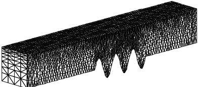
Fig. 12 Illustration of initial mesh for scattering problems due to periodic bars

The two cases to be considered are the same as those in [37], i.e., bar patches with 4 and 10 sinusoidal bars on the seabed, respectively. The wave generator motions are as specified by Eq. (25). For ease of description, the side of the bar patch near the wavemaker is called the front side, and the other side the lee side. The initial meshes used are similar to that illustrated in Fig. 12 but much finer. The reflection coefficients, defined by Kr = Ar/Ai, where Arand Ai are the amplitudes of reflecting and

incident waves, are calculated from wave histories recorded at a series of points along the tank by using the same method as in [37], in which it is assumed that the wave consists of incident and reflected waves with the same frequencies. It should be noted that for the purpose of computing the reflection coefficients, the time history to be used at a point must start from the time when the wave reflected from the lee side has arrived at the point and end before the wave reflected from the front side travels back to the point after interacting with the wavemaker. Otherwise, either the reflecting waves are not fully developed at the point or affected by the re-reflecting waves from the wavemaker. The start (tst) and end (tend) times may be estimated by

g bp wp

st

L

L

C

t

=

(

+

2

₂

)

/

(27a)

g bp wp

end

L

L

C

t

=

(

3

+

2

₁

)

/

(27b)

where is the group velocity of the water wave; is the distance from the wavemaker to the point considered; and are the distances from the point to the front and lee sides of the bar patch, respectively.

g

C

L

_wp

1 bp

L

L

_bp2

respectively as ab/d = 0.32 for 4 bars and ab/d = 0.16 for 10 bars. The wave histories recorded at two

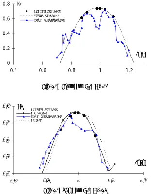
points about 5 bar-lengths before the front side of the bar patch are used. Reflection coefficients near the resonant condition (2k/kb = 1, where k is the water wave number) are presented in Fig. 13 together

[image:20.595.143.457.336.738.2]

with experimental data from [37]. For the case with 10 bars, the nonlinear numerical results from [41] and analytical results from the simplified model [38] are also included. For the case with 4 bars, the analytical results from [40] are plotted apart from the experimental and our numerical results. From Fig. 13a for this case, it can be seen that the numerical results obtained by using the QALE-FEM method agree well with the analytical results given in [40] and satisfactorily with experimental data in [37]. Fig. 13b for 10 bars indicated that our numerical results are almost identical to those from [41] and closer to the experimental data than the analytical solution based on the simplified model [38] on the side of 2k/kb >1. On the side of 2k/kb <1, our results differ slightly from [41] but are closer to the

experimental data in [37] and the analytical results from the simplified models [38].

0 0.2 0.4 0.6 0.8

0.4 0.6 0.8 1 1.2

2k/kb

Kr

QALE-FEM numerical Port er & Port er [ 40] David & Heat hershaw [ 37]

Fig. 13a Four bars, ab/d = 0.32

0.0 0.2 0.4 0.6 0.8

0.8 0.9 1 1.1 1.2

2k/kb

Kr

QALE-FEM numerical Liu & Yue [ 41] David & Heat hershaw [ 37] Mei [ 38]

Fig. 13b Ten bars, ab/d = 0.16

Fig. 13 Reflection coefficients (Kr =Ar/Ai with Ar and Ai being the amplitudes of reflection and incident

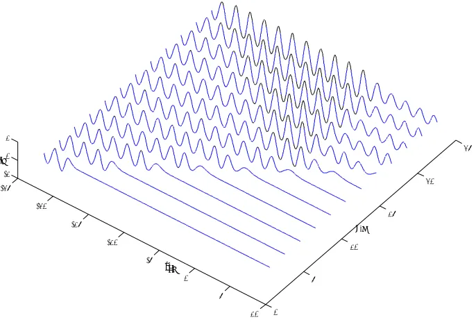
[image:20.595.149.447.341.494.2]

To further show the properties of the reflected waves, the wave profiles at different instants for 4 bars are plotted in Fig. 14, in which the coordinate system is shifted so that its origin is at the centre of the bar patch, and the bar patch is located in the range of −2<x/λ_b <2(λ_b =2π/k_b). It can be observed that when the incident wave reaches the bars, the reflected wave begins to be produced. The reflected wave propagates towards the wavemaker, is superimposed onto the incident wave and makes the resultant wave before the front side (

x

/

λ

_b

=

−

2

) higher than the incident wave. It can also be observed that the wave after the lee side (

x

/

λ

_b

=

2

)

is considerably smaller than the wave before the front side, as expected.

-25

-20

-15

-10

-5

0

5

10 0 5

10 15

20 25

-1 0 1

/T τ

b λ x/ /a

[image:21.595.134.477.275.507.2]

ζ

Fig. 14 The wave profiles at different instants for 4 bars

0 0.2 0.4 0.6 0.8

-10 -5 0 5

Kr

Measured Analytical a=0.04 a=0.12 a=0.192

0.50 0.60 0.70 0.80

0 0.05 0.1 0.15 0.2

a

Kr

(a) Kr at different positions (b) Kr at x/λb ≈−4

[image:21.595.85.513.581.732.2]

In order to investigate the nonlinear effects, the case with 4 bars is simulated with different amplitudes. All other parameters except for the amplitude are the same as those for Fig. 13. The reflection coefficients corresponding to 2k k_b ≈1 are presented in Fig. 15. In Fig. 15a, the coefficients at different positions are plotted together with the experimental results and analytical solution from [37]. It can be seen that the reflection coefficients are close to the linear analytical solution when the amplitude is small but close to the measured data when the amplitude is larger. In addition, the reflection coefficients before the front side (

x

/

λ

_b

=

−

2

) tend to decrease with the increase of the amplitudes, though the reduction is not very significant. To further show this trend, the numerical reflection coefficients at a point x/λb= -4 are plotted in Fig. 15b. It should be noted that the

method for estimating the reflection coefficients is the same as in Fig. 13 in order to compare the results with those in [37]. However, when the nonlinearity becomes strong, high-order waves are involved. The reflection coefficients found in this way correspond only to the wave with the same frequency as the first order wave and do not include the reflection of high-order waves.

In order to look at overall reflection of nonlinear waves by the bar patch, the shapes of wave profiles for the same case are illustrated in Fig. 16. In this figure, the wave profiles for smaller and larger amplitudes are depicted to show the different reflection properties. As can be seen, the wave profiles on the left of the bar patch for the smaller amplitude seems to be formed by superimposing two harmonic waves with the same length travelling in opposite directions (so the wave become higher) but the shape is still similar to that of harmonic waves. For the larger amplitude, the wave amplitude on the left of the bar batch seems not to be changed dramatically by the reflection waves, instead, the shape of the waves is significantly modified.

-25 -20 -15 -10 -5 0 5 10

-1 -0.5 0 0.5 1

x/λb ζ/a τ=15T

-25 -20 -15 -10 -5 0 5 10

-1 -0.5 0 0.5 1

x/λb ζ/a τ=20T

-25 -20 -15 -10 -5 0 5 10 -1

-0.5 0 0.5 1

x/λb

ζ/a τ=15T

-25 -20 -15 -10 -5 0 5 10

-1 -0.5 0 0.5 1

x/λb

ζ/a τ=20T

[image:23.595.145.458.74.232.2]

(b) a=0.192

Fig. 16 Wave profiles corresponding to different amplitudes for 4 bars

6. QUALITY OF MESH DURING SIMULATION AND EFFICIENCY OF MESH MOVING

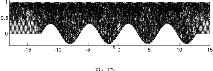
A significant development in this paper is to move, instead of re-generating, the unstructured mesh at every time step when simulating water waves based on the FNPT Model. As pointed out in Section 3, the mesh obtained should have satisfactory element shapes and preserve the reasonable refinement and distribution in regions of interest, such as those close to the free surface and the bars on the tank-bed at all time steps. In order to show the quality of mesh moved by using the method discussed in Section 3, Fig. 17 and Fig. 18 are presented for a case with 4 bars. Fig. 17a shows a part of the initial unstructured mesh while Fig. 17b illustrates the enlarged mesh in areas near the two sides of the bar patch. Fig. 18 depicts the corresponding part of the mesh at about τ = 332. These figures demonstrate that the original refinement and distribution are kept and all elements are of satisfactory shape after long time simulation. In addition, negative elements, which are of concern when using the linear spring analogy method, do not appear in the simulation. This implies that the techniques used for moving mesh described in Section 3 work very well. Nevertheless, certain changes in the sizes and shapes of individual elements are observed and expected because the fluid domain varies with propagation of waves. It is these changes that make it possible to conform to the moving boundaries at all time steps and so to achieve satisfactory results as demonstrated in Section 5.

-15 -10 -5 0 5 10 15

0 0.5 1

x

z

[image:23.595.113.486.595.721.2]

-15 -14 -13 -12 -11 -10 -9 0

0.5 1

z

x _{8 9 10 11 12 13}

0 0.5 1

z

x

Fig. 17b

Fig. 17 Initial mesh for 4 bars

-15 -10 -5 0 5 10 15

0 0.5 1

x

z

Fig. 18a

-15 -14 -13 -12 -11 -10 -9

0 0.5 1

z

x _{8 9 10 11 12 13}

0 0.5 1

z

x

[image:24.595.85.493.75.530.2]

Fig. 18b

Fig. 18 Mesh at τ ≈332 (4 bars, a=0.192 )

same case had been simulated using a conventional FEM with the same mesh regenerated at each time step, the total CPU time on each time step would have been about 60s. This implies that the QALE-FEM requires less than 15% of the CPU time required by the conventional QALE-FEM. It should be noted that the time spent on adjusting nodes on the free surface depends on how often it is undertaken. Its frequency depends on the number of time steps used each period and the wave steepness. The more time steps in each period, the less frequently adjustment has to be performed. On the other hand, the steeper the waves, the more often adjustment is needed. According to our experience so far, the adjustment frequency is unlikely to be less than every ten time steps if a reasonable time step is chosen. Even with a frequency of every ten time steps to adjust the nodes on the free surface, the CPU time required by using the QALE-FEM is still considerably less than that by the conventional FEM. Therefore, it can be confidently stated that the QALE-FEM is much faster than the conventional FEM when using unstructured meshes.

7. CONCLUSION

In this paper, the QALE-FEM is developed to simulate nonlinear water waves based on the FNPT Model. In this method, the boundary value problem about the velocity potential is solved by using a finite element method and the mesh is moved in order to conform to the wavy free surface and other moving boundaries. The method allows the efficient use of unstructured meshes without the need to regenerate it at every time step, which is a necessary and very costly feature of the conventional FEM. To achieve overall high efficiency and accuracy, several numerical techniques involved in the QALE-FEM have been developed, including the method to move interior nodes, the technique to re-distribute the nodes on the free surface, the scheme to compute velocities, and so on.

The newly developed method has been validated by comparing its numerical predictions with published analytical solutions, experimental data and results from other methods. The validation cases included the monochromatic, bichromatic and random waves and also included the interaction between waves and periodic bars on the seabed. In all cases, the results given by the present method agree well with published data. Assessments are made on the efficiency of moving mesh and quality of elements obtained by moving the mesh, which shows that unstructured mesh quality is satisfactorily maintained and the QALE-FEM requires only a small fraction of CPU time that would be spent on using the conventional FEM if unstructured mesh is used.

Although the newly developed method is applied only to problems without floating bodies in this paper, it is not very difficult to extend it to deal with problems with floating bodies. When floating bodies are involved, the nodes on the body surfaces may be adjusted in a way similar way to that for the free surface.

8. ACKNOWLEDGEMENT

authors also thank Dr Ping Dong, Dundee University, UK, for him bringing the problem about periodic bars to our attention.

9. REFERENCE

[1] Greaves, DM, Simulation of interface and free surface flows in a viscous fluid using adaptive quadtree grids, Int. J. Numer. Meth. Fluids, 44 (2004), 1093-1117.

[2] C. Hirt, B. Nichols, Volume of fluid (VOF) method for the dynamics of free surface boundaries, J. Comput. Phys., 39 (1981) 210–225.

[3] S. Navti, R. Lewis, C. Taylor, Numerical simulation of viscous free surface flow, Int. J. Numer. Methods Heat Fluid Flow, 18(1998) 445–464.

[4] Yue, W., Lin, C.L., Patel, V.C., Numerical simulation of unsteady multidimensional free surface motions by level set method, Int. J. Numer. Meth. Fluids, 42(2003) 853-884.

[5] Donea, J., Fasoli-Stella, P., Giuliani, S., Finite element solution of transient fluid-structure problems in Lagrangian coordinates, Proceedings of the International Meeting on Fast Reactor Safety and Related Physics, Chicago, 3(1976), 1427–1435.

[6] Fabián Duarte, Raúl Gormaz, Srinivasan Natesan, Arbitrary Lagrangian–Eulerian method for Navier–Stokes equations with moving boundaries, Computer Methods in Applied Mechanics and Engineering, 193( 2004), 4819-4836.

[7] Henning Braess, Peter Wriggers, Arbitrary Lagrangian Eulerian finite element analysis of free surface flow, Comput. Methods Appl. Mech. Engrg. 190 (2000), 95-109.

[8] Souli, M., Zolesio, J.P., Arbitrary Lagrangian–Eulerian and free surface methods in fluid mechanics, Comput. Methods Appl. Mech. Engrg., 191(2001), 451-466.

[9] Lachaume, C., Biausser, B., Grilli, S. T., Fraunie, P., Guignard, S., Modeling of Breaking and Post-breaking Waves on Slopes by Coupling of BEM and VOF Methods, Proceedings of the International Offshore and Polar Engineering Conference, 2003, 1698-1704.

[10] Clauss G.F., Steinhagen U., Numerical simulation of nonlinear transient waves and its validation by laboratory data, Proceedings of the 9th International Offshore and Polar Engineering Conference, Brest, France, 1999, 368-375.

[11] Ma, Q.W., Wu, G.X., Eatock Taylor, R., Finite element simulation of fully non-linear interaction between vertical cylinders and steep waves. Part 1: Methodology and numerical procedure, Int.J.Numer. Meth. Fluids,36(2001), 265-285.

[12] Ma, Q.W., Wu, G.X., Eatock Taylor, R., Finite element simulation of fully non-linear interaction between vertical cylinders and steep waves. Part 2: Numerical results and validation, Int.J.Numer. Meth. Fluids, 36(2001), 287-308.

[13] Longuet-Higgins, M.S., Cokelet, E.D., The deformation of steep waves on water: I. a numerical method of computation, Proc. R. Soc. Lond. A 350 (1976), 1–26.

Res. 42 (1998), 33–45.

[15] Grilli, S.T., Guyenne, P., Dias, F., A fully nonlinear model for three-dimensional overturning waves over arbitrary bottom, Intl J. Numer. Meth. Fluids, 35(2001), pp. 829-867.

[16] Cao, Y., Schultz, W.W. & Beck, R.F., Three-dimensional desingularised boundary integral method for potential problems, Int. J. Num. Meth. Fluids, 12(1991), 785-803.

[17] Wang, P., Yao, Y., Tulin, M., An efficient numerical tank for nonlinear water waves, based on the multi-subdomain approach with BEM, Int. J. Num. Meth. Fluids, 20(1995), 1315-1336.

[18] Wu, G.X., Eatock Taylor, R., Finite element analysis of two dimensional non-linear transient water waves, Appl. Ocean Res. 16(1994), 363–372.

[19] Wu, G.X., Eatock Taylor, R., Time stepping solution of the two dimensional non-linear waveradiation problem, Ocean Eng. 22(1995), 785–798.

[20] Cai, X., Langtangen, H.P., Nielsen, B.F., Tveito, A., A finite element method for fully nonlinear water waves, J. Comp. Physics, 143(1998) 544-568.

[21] Westhuis, J.H., Andonowati , Applying the finite element method in numerically solving the two dimensional free-surface water wave equations, 13th _{International Workshop on Water Waves and}

Floating Bodies, Alphen aan den Rijn, The Netherlands, 1998; 171-174.

[22] Wu, G.X., Hu, Z.Z., Simulation of nonlinear interactions between waves and floating bodies through a finite-element-based numerical tank, Proceedings A of the Royal Society, 460 (2004), No. 2050, 3037-3058.

[23] Heinze, C., Nonlinear hydrodynamic effects on fixed and oscillating structures in waves, PhD Thesis, Department of Engineering Science, Oxford University, 2003.

[24] Ma, Q.W., Numerical simulation of nonlinear interaction between structures and steep waves, PhD Thesis, Department of Mechanical Engineering, University College London, UK, 1998.

[25] Aymone , J.L.F., Bittencourt , E., Creus, G.J., Simulation of 3D metal-forming using an arbitrary Lagrangian-Eulerian finite element method, Journal of Materials Processing Technology, 110 (2001), 218-232.

[26] Gadala, M. S., Recent trends in ALE formulation and its applications in solid mechanics, Computer Methods in Applied Mechanics and Engineering, 193(2004), 4247-4275.

[27] L¨ohner R, Yang C., Improved ALE mesh velocities for moving bodies. Commun. Numer. Methods Eng., 12(1996), 599–608.

[28] Batina, J. T., Unsteady Euler Airfoil Solutions Using Unstructured Dynamic Meshes, AIAA Paper 89-0115, 27th AIAA Aerospace Sciences Meeting, January, 1989.

[29] Anderson, W. K., Aerodynamic Design Optimization on Unstructured Grids with a Continuous Adjoint Formulation, AIAA Paper 97-0643, 35th AIAA Aerospace Sciences Meeting, January 1997.

Portland, Oregon, June 2004.

[31] Degand, C, Farhat, C., A three-dimensional torsional spring analogy method for unstructured dynamic meshes, Computers & Structures, 80(2002), 305-316.

[32] Bottasso, C.L., Detomi, D., Serra, R., The ball-vertex method: a new simple spring analogy method for unstructured dynamic meshes, to appear on Computer Methods in Applied Mechanics and Engineering, 2004.

[33] Frey, P. J. , Borouchaki H., George P., 3D Delaunay mesh generation coupled with an advancing-front approach, Computer Methods in Applied Mechanics and Engineering, 157 (1998), 115-131. [34] Davies, Carol B., Venkatapathy, Ethiraj, SAGE: The Self-Adaptive Grid Code, Version 3,

NASA/TM-1999-208792 (1999).

[35] S.N. Atluri, T. Zhu, A new meshless local Petrov-Galerkin (MLPG) approach in computational mechanics, Computational Mechanics, 22 (1998), 117-127.

[36] Heathershaw, A.D., Seabed-wave resonance and sand bar growth. Nature, 296 (1982), 343-345. [37] Davies, A.G., Heathershaw, A.D., Surface-wave propagation over sinusoidally varying topography,

J. Fluid Mech, 144 (1984), 419-440.

[38] Mei, C.C., Resonant reflection of surface water waves by periodic sandbars, J. Fluid Mech., 152(1985), 315-335.

[39] Chamberlain, P. G., Porter, D., The modified mild-slope equation, J. Fluid Mech., 291 (1995),393–407.

[40] Porter, P., D.Porter, D., Scattered and free waves over periodic beds, J. Fluid Mech., 483(2003), 129–163.

[41] Liu, Yuming, Yue, Dick K. P., On generalized Bragg scattering of surface waves by bottom ripples, J. Fluid Mech., 356(1998), 297-326.

[42] Eatock Taylor, R, Wang, B.T., Wu, G.X., On the transient analysis of the wavemaker, 9th

International Workshop on Water Waves and Floating Bodies, Kuju, Oita, Japan, 1994.

[43] Nestegard, A., Status of Nonlinear hydrodynamic modelling, Technical report, DNV, Norway, 1999.

Dr. Qingwei Ma Senior Lecturer in Fluids Engineering School of Engineering and Mathematical Science City University Northampton Square London EC1V 0HB, UK T el. 0044 20 7040 8159 Fax 0044 20 7040 8566 31/05/2005

Re: JCOMP-D-05-00185

Quasi ALE finite element method for nonlinear water waves

Dear Editor,

The enclosed are the revised version of the above paper.

Some minor changes have been made in this version based on the suggestions of two

reviewers. In addition, some typing errors identified ourselves are also corrected.

We list the detailed responses to the referee’s comments and corresponding changes

on separate pages enclosed with this letter.

Yours sincerely

Qingwei M a

Responses to the comment of Reviewer

####

1

We are grateful for the reviewer to identify that the article is well written and the

results is interesting.

The following are our reply to reviewer’s questions and comments:

1) The authors should comment on the solid boundary, I think it is difficult if the rigid

boundary is not a simple wall. There will be singularity at the intersection point (free

surface and rigid boundary).

It is right to say that there exists singularity at the intersection point. Various

techniques have been suggested to eliminate the problem, as reviewed in [24]. These

techniques may have different forms for different numerical methods used. With the

finite element method, Wu and Eatock Taylor [44] have found that singularity

problem at the waterline can be suppressed by simply using the form as given in Eq.

(7) in this paper. To reflect this, two more sentences are added below Eq. (7).

2) The velocity on the free surface will only have first order accuracy when the

authors use linear elements, is it enough for this problem?

We agree with the reviewer that the velocity have only first order accuracy because

the linear element is used. Enhancing accuracy may be achieved either by using the

high order elements or the finer mesh. To use high order elements leads to intricate

integration on each element and requires more CPU time on the element analysis.

Therefore, in our previous papers (e.g. [11]and [12] in the Reference), we choose to

use linear elements and validated various cases with published data. In this paper,

the model is validated using more experimental data and satisfactory agreement

achieved. Based on these validations, we could say that linear element is one of

choices which could give satisfactory results.

3) Please comment on the mesh which seems not uniform. How to assure the accuracy

of the method?

There are several ways to assure the accuracy of the method, such as comparing

results with published numerical and experimental data, simulating same cases with

different number of elements and different distribution of elements, applying the same

method to different cases under various conditions and so on. As presented in Section

5, the newly developed method has been used for various cases and validated in

different ways. We believed that the method should be considered to have satisfactory

accuracy based on the results presented.

4) As the authors point out, the mesh near the free surface and corner should be more

fine, how to do that?

As indicated in Section 3, the reasonable distribution of elements is achieved by

generating satisfactory initial mesh. The satisfactory distribution is maintained when

moving the mesh at all time steps by using the reasonable spring stiffness, such as

given in Eqs. (13) and (21).

5) Equation (21) needs explanation.

More explanation is added below the equation.

6) Page 14, "t = 5T and 15T", should be "t = 10T and 15T"?

Yes, it should. This is now rectified

7) Page 22: "CUP" -> "CPU"

This is now rectified

8) In Figures 17 and 18, the mesh seems not uniform and the changing from

sparseness to denseness is a little sharp. This needs more explanation.

These two figures illustrate the mesh at

τ

=0 and the mesh after long time

simulation (

τ

= 332). They demonstrate that the techniques used for moving mesh

Responses to the comment of Reviewer

####

2

We are grateful for the reviewer to identify that the paper makes important

contribution in developing new method.

The following are our reply to reviewer’s questions and comments:

1) I would demand is to include the time-stepping algorithm used for the boundary

conditions on the surface, i.e., equations (2) and (3). It is not clear how these

conditions are treated discretely in the proposed QALE formulation.

The time-stepping algorithm is the same as in [11] and also similar to that in [13].

The main difference between QALE-FEM and conventional FEM in [11] is that the

mesh is moved rather than re-generated. For ease of understanding, we take the

point of the reviewer and change “

to update the position of and the potential values on the

free surface

” into “

to update the position of and the potential values on the free surface using the same method as in [11]

” in the paragraph below Eq. (5)

2) I could also wish convergence rates of the method were computed, but the quality

of the numerical verification/validation section is high as it stands.