A Geometric Test for the Analysis of Contingency Tables
J. Quigley & K.J. Wilson
Department of Management Science, University of Strathclyde, UK
ABSTRACT: The Chi-squared test for contingency tables has good performance when sample sizes are suf-ficiently large but is not appropriate with small samples. When this condition is violated, Fisher’s exact test is often used as it is valid for all sample sizes. However, Fisher’s test has been criticised for being overly con-servative. Alternatives have been proposed but typically involve more complex computations. In this paper we propose an alternative test based on a geometric projection of the multinomial distribution onto the n-sphere. Each multinomial observation is represented by a single point on this sphere. The angle between two points rep-resenting two different multinomial observations can then be compared to the distribution of the angle under the assumption that the realisations come from the same underlying distribution. The null hypothesis distribution is simulated and easy to compute. This new test is compared to the Chi-Squared test and Fisher’s Test in terms of both Type I and Type II errors and its potential use in reliability modelling is indicated using a real case study.
1 INTRODUCTION
Contingency tables are widely used in the areas of safety and reliability modelling when there are several machines, systems or failure types which are possibly spread over different locations. Typically we wish to know whether there are differences between the prob-ability of failure between the different states of two of the different factors such as failure type and lo-cation. Examples include (Conte, Rubio, Garcia, & Cano 2011, Maiti & Khanzode 2009, Colombo & Ihm 1988, Schneidewind 1992).
Conte et al. (Conte, Rubio, Garcia, & Cano 2011) considered a19×19risk-injury contingency table of the accident rates in Spanish companies over an 11 year period to identify separate risk and injury groups. Maiti and Khanzode (Maiti & Khanzode 2009) inves-tigated a relative risk model using a two way contin-gency table for fatal roof and side fall accidents at coal mines in India.
In Colombo and Ihm (Colombo & Ihm 1988) fail-ure rates at nuclear power plants were considered. The failure rates of components were broken down by plant location and reactor system. This led to a con-tingency table for the numbers of failures which was further complicated by the different exposures at each of the plants. Schneidewind (Schneidewind 1992) was interested in the validation of software metrics. His proposed methodology used contingency tables as an important part of this validation process, counting up the numbers of correct and incorrect classifications of each type.
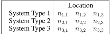
An example of a contingency table, based on the two factors in Colombo and Ihm (Colombo & Ihm 1988), is given in Table 1.
Location System Type 1 n1,1 n1,2 n1,3
System Type 2 n2,1 n2,2 n2,3
[image:1.595.342.529.439.497.2]System Type 3 n3,1 n3,2 n3,3
Table 1: An example contingency table with factors Location and System.
In such a contingency table we would typically be interested in whether there were differences in the probabilities or rates of failures which result in the ob-served numbers of failures ni,j, i, j = 1,2,3between
the different locations or systems. There are two main statistical tests which could be used to do this; the Chi-Squared Test and Fisher’s Exact Test (Pearson 1900, Fisher 1922).
In the Chi-Squared test expected frequencies are calculated for each of the cells in the contingency ta-ble ei,j and these are then compared to the observed
frequencies to form the Chi-Squared test statistic
χ2 =
I
X
i=1
J
X
j=1
(ni,j−ei,j)2
e2
i,j
,
which is compared to the χ2 distribution on (I −
when at least one of the frequencies is smaller than this (Cochran 1954). It cannot be carried out with multiple observed frequencies of 0.
Variants to the Chi-Squared Test have been pro-posed for small sample sizes. Two of the most promi-nent are the Yates correction and Fisher’s Test. In Fisher’s Test an exact p-value is calculated based on the assumption that the row and column totals are fixed. While the Fisher Test is exact and so is suit-able for small sample sizes it has been criticised for being overly conservative (Liddell 1976). This con-servatism stems from the discrete nature of the test statistic and the assumption of fixed marginals. Sev-eral other variants have been proposed in the literature but many of these rely on intensive numerical meth-ods and are therefore, for practitioners wishing to test for differences quickly and simply, not always suit-able or appropriate.
(Olbrich 1965) proposed a geometric projection of the multinomial distribution onto the n-sphere. Each multinomial observation was represented by a single point on this sphere and the difference between two multinomial realisations of the same degree was rep-resented by the angle between the two points on the sphere. This representation had the nice property that it was variance stabilising. The representation was not commutative, however; if the order of the categories were switched in the multinomial distributions then the points on the sphere and the angle between the points did not remain the same.
In this paper we propose a commutative version of the (Olbrich 1965) representation. We then use this version to define a hypothesis test to test for differ-ences in contingency tables. The test statistic is the angle between the two multinomial realisations. We use the variance stabilising property of the transfor-mation in order to approximate the distribution un-der the null hypothesis that the two realisations come from the same underlying probability vector. The test does not require intensive numerical methods.
The remainder of the paper is structured as follows. In Section 2 we review the method of (Olbrich 1965), give our proposed commutative adaption and outline the geometric hypothesis test. In Section 3 we inves-tigate the properties of the proposed transformation and in Section 4 we conduct a simulation study to as-sess the performance of the Geometric Test against the Chi-Squared Test and Fisher’s Test for both Type I and Type II errors. Finally, in Section 5 we give an illustrative example of the method and we conclude the paper in Section 6.
2 GEOMETRIC TRANSFORMATION OF
MULTINOMIALS
2.1 The Olbrich Transformation
Consider two realisations from a multinomial distri-bution inndimensions,(x1, . . . , xn)and(y1, . . . , yn).
Let
xT =
n
X
i=1
xi, yT =
n
X
i=1 ,
be the total number of observations from each of these multinomials. Then the proportions of the observa-tions in each of the categories are
pi=
xi
xT
, qi=
yi
yT
.
Olbrich proposed representing the multinomials in spherical co-ordinates as points on an n-shphere using these proportions. Denote these points byθ, φ respec-tively. Then
θ = (cos−1(√p1), . . . ,cos−1(
√
pn)),
φ = (cos−1(√q1), . . . ,cos−1(
√
qn)).
We can use such a transformation to calculate the an-gle between any two multinomial realisations on the n-sphere. This is given in the below result.
Theorem 1. The angleAObetween two multinomial
realisations(x1, . . . , xn)and(y1, . . . , yn)with
propor-tions of observapropor-tions in each categorypi =
xi
xT
, qi =
yi
yT
is given by
AO= cos−1
n+1
X
i=1
v u u tpiqi
"i−1 Y
j=0
(1−pj)(1−qj)
# ,
wherep0 =q0 = 0, andp1=q1 = 1.
Proof. We can represent these points in Cartesian co-ordinates in(n+ 1)dimensions. That is,
c1 = rcos(cos−1(
√
p1)),
c2 = rcos(cos−1(
√
p2)) sin(cos−1(
√
p1)),
.. .
cn = rcos(cos−1(
√
pn))
n−1
Y
i=1
sin(cos−1(√pi)),
cn+1 = r
n
Y
i=1
sin(cos−1(√pi)).
The radius is r = q
Pn+1
i=1 c 2
i. This representation
√
1−z2, to
c1 = r
√
p1,
c2 = rpp2(1−p1),
.. .
cn = r
v u u tpn
n−1
Y
i=1
(1−pi),
cn+1 = r
v u u t n Y i=1
(1−pi).
We denote the Euclidian co-ordinates for θ as
(c1(θ), . . . , cn+1(θ))and forφas(c1(φ), . . . , cn+1(φ)).
Then the angle between these two points is
AO= cos−1
Pn+1
i=1 ci(θ)ci(φ)
q Pn+1
i=1 ci(θ)2
Pn+1
i=1 ci(φ)2
.
This reduces to the result given.
The angle has the nice property that it tends to zero for two multinomial realisations from the same under-lying distribution as the sample sizes go to infinity. To see this, consider
lim
xT,yT→∞
A = cos−1
1−ρn+ n X i=1 v u u tρ2i
i−1
Y
j=1
(1−ρj)2
= cos−1 1−ρn+ n
X
i=1
ρi
i−1
Y
j=1
(1−ρj)
!
= cos−1(1) = 0.
2.2 The Commutative Property
Upon inspection of the angle,AO, in Theorem 1, it is
apparent that the choice of label, i.e.,i, which a cate-gory is assigned will influence the resulting value of the angle. That is, if the categories of the multinomial variables are re-ordered, then the angle between them using the Olbrich transformation will be different.
Consider a simple 2×2 table with the two cate-gories being “blue” and “not blue”. Here the test statistic reduces to one of the two following test statis-tics depending on which category is assigned to be the first category.
aO = cos−1(
√
pblueqblue+ (1−pblue)(1−qblue))
6
= cos−1p(1−pblue)(1−qblue) +pblueqblue
.
This non-commutative property is a result of the dependence structure in the probabilities which en-sures that they sum to 1 over all categories. As such, if we re-define the probabilities used within the test such that they are conditionally independent then we will have a commutative representation of the angle between two multinomial realisations.
As such, by using probabilities conditionally inde-pendent on categories with a lower index value and following the same geometric transformation as in Ol-brich’s work we can obtain a commutative formula for the angle. This is given in the following theorem. The proof follows the same form as that for Theorem 1. It is left to the reader.
Theorem 2. The angleAGbetween two multinomial
realisations(x1, . . . , xn)and(y1, . . . , yn)with
condi-tional proportions of observations in each category given that they weren’t in any previous categories
γi =
xi
xTi
, βi =
yi
yTi
, where XTi =
Pn
j=ixj, YTi =
Pn
j=iyj, is given by
AG = cos−1
n+1 X i=1 v u u tγiβi
"i−1 Y
j=1
(1−γi)(1−βi)
#
= cos−1
n
X
i=1
√
piqi
!
,
wherep0 =q0 = 0, andp1=q1 = 1.
2.3 Geometric Hypothesis Test
Suppose we have two multinomial realisationsxand
ywith underlying probability vectorspandq respec-tively. We wish to test whether the two vectors come from the same underlying multinomial distribution. The hypothesis test will take the form
H0: p=q,
H1: p6=q.
The test statistics is
AG= cos−1
v u u t n X i=1 ˆ
piqˆi
,
for observed pˆi = xi/xT,qˆi =yi/yT. The p-value is
then
Pr(a≥AG)≈
1
N
N
X
i=1
I(ai≥AG),
where N is a large number of simulated values of
a1, . . . , aN we need to estimate the probability vector
under the null hypothesis,p
0. This is
ˆ
p
0 =
1
2×(ˆp1+ ˆp2).
Thus we see that to perform the test we carry out a parametric bootstrap (Efron & Tibshirani 1993) onp0.
3 PROPERTIES OF THE TRANSFORMATION We have evaluated the mean and standard deviation of the angleAGresulting from the transformation of one
multinomial variable compared with its mean. The aim is to develop some intuition concerning the be-haviour of this transformation. We have considered the mean and standard deviation with respect to the underlying probabilities and sample size.
[image:4.595.360.505.125.261.2]Specifically, we have used Maple 17 software to calculate the mean and standard deviation exactly for multinomial distributions with 3 to 10 categories. In varying the underlying probabilities we used the stan-dard deviation of the probabilities, as this is related to the Euclidean distance of the vector of probabilities from the vector of equal probabilities. Our standard deviations range from 0 to 0.5. We give two figures below to illustrate the analysis. The overall conclu-sions made are based on the more comprehensive in-vestigation.
Figure 1: Mean and standard deviation ofAG form= 3with
standard deviations of 0 (left) and 0.29 (right).
In Figure 1 we see the change in the mean and standard deviation ofAG for a 3-dimensional
multi-nomial distribution over different sample sizes. In the left hand plot the standard deviation is 0 and in the right hand plot it is 0.29. In Figure 2 we see the same two plots for a 10 dimensional multinomial distribu-tion.
Figure 2: Mean and standard deviation ofAGform= 10with
standard deviations of 0 (left) and 0.29 (right).
An interesting pattern in the mean of angle from the transformation is that it monotonically decreases as sample size increases. Our study considered 99 dif-ferent combinations of probabilities, number of cate-gories and sample sizes, from which we are able to
a
Frequency
0.0 0.2 0.4 0.6 0.8
0
1000
a
Frequency
0.00.20.40.6
0
1000
a
Frequency
0.00.2 0.40.6
0
1000
a
Frequency
0.0 0.20.4 0.6
0
1000
a
Frequency
0.0 0.2 0.4 0.6
0
1000
a
Frequency
0.0 0.2 0.4 0.6
0
1000
a
Frequency
0.0 0.20.4 0.6
0
1000
2500
a
Frequency
0.0 0.2 0.4 0.6
0
1000
2500
a
Frequency
0.0 0.2 0.4
0
1000
[image:4.595.45.281.421.492.2]2500
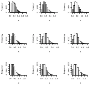
Figure 3: The distribution ofAGfor 10,000 simulated pairs from
the trinomial distribution with the same probability vector.
fit a curve to the relationship between the mean an-gle, the standard deviation of the probabilities and the number of samples. That is,
¯
xA= 1.356−2.8×sp+ (0.8×sp−0.34) log(n),
where x¯A is the mean of AG and sp is the standard
deviation of the probabilities. This excludes the cases with equal probability. The fit of the curve was very good with R2 = 87.8%, and it shows that the mean
decreases at a rate o(log(n)) and is not affected by the number of categories m. The standard deviation of the probabilities influences the mean in two ways; it decreases the mode and increases the rate of decay with respect to sample size.
4 SIMULATION STUDY 4.1 The distribution ofAG
We wish to compare two multinomial realisations to test if they come from the same underlying distribu-tion, i.e., if the have the same probability vector.
In Figure 3 we give histograms of the angleAGfor
the trinomial distribution simulated with the same un-derlying probabilities for a range of different param-eter vectors. In each case 10,000 pairs of points are simulated and there are 50 observations for each sim-ulated point.
We see that in all cases the distribution ofAG has
[image:4.595.50.274.631.702.2]a
Frequency
0.8 1.2
0
1000
a
Frequency
0.2 0.6 1.0
0
1000
a
Frequency
0.00.20.40.6
0
1000
a
Frequency
0.6 1.0 1.4
0
1000
a
Frequency
0.2 0.4 0.6 0.8
0
1000
a
Frequency
0.0 0.2 0.4
0
1500
a
Frequency
0.4 0.8 1.2
0
1000
a
Frequency
0.0 0.20.40.6
0
1000
a
Frequency
0.0 0.20.4 0.6
0
[image:5.595.85.229.127.263.2]1000
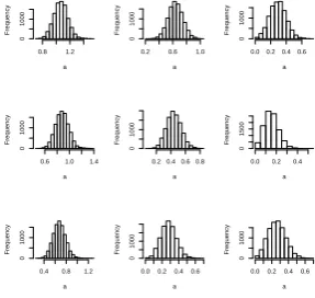
Figure 4: The distribution ofAGfor 10,000 simulated pairs from
the trinomial distribution with different probability vectors.
We can carry out a similar simulation exercise for trinomial realisations which come from distributions with different underlying probability vectors. The re-sulting histograms are given in Figure 4. Again, each graph is the result of 10,000 simulations.
This time we see that the distributions of AG are
generally much more symmetric and have modes which are typically larger than in Figure 3. This sug-gests thatAGmay be a useful statistic within the
hy-pothesis test we have outlined in Section 2.3.
4.2 Type I and Type II errors
We will investigate the properties of the test with re-spect to Type I and Type II errors. All results are based on 1000 samples. The Type I error probabili-ties are given in Table 3 in the Appendix for two dif-ferent probability vectors and difdif-ferent sample sizes. The probabilities from the Pearson Chi-squared test are also given.
We see that, for p
1 and p2 all three tests are
per-forming fairly well, with the proportions of Type I errors being close to 0.05 for all tests over almost all sample sizes. This indicates that, for trinomials in which all of the categories have reasonably large probabilities, all of the tests perform satisfactorally with respect to Type I errors. However, forp
3in which
there are small probabilities of being in some of the categories and hence small numbers of observations in those categories, all three tests have proportions of Type I errors well below 0.05 for a sample size of 5. The geometric test then performs well from a sample
size of 10 whereas the other two tests are still making too few Type I errors up to a sample size of approxi-mately 30.
The Type II errors are given in Table 4 in the Appendix. In Table 4 probabilities are p
1 =
(1/3,1/3,1/3), p
2 = (1/2,1/4,1/4) and p3 =
(8/10,1/10,1/10).
We see that the Geometric Test outperforms the other two tests for all combinations of probability vec-tors for sample sizes of 5 and 10. Beyond a sample size of 10 the Fisher Test, in particular, typically out-performs the Geometric Test. However, in this paper we are interested in situations where we have small probabilities and possibly few data and the in this case the Geometric Test give an improvement, albeit small, over the other two tests. When combined with its superior Type I error probabilities for the trinomial distribution with low probability events and this new Geometric Test looks to have some strengths over the two traditional tests.
5 ILLUSTRATIVE EXAMPLE
The illustrative example in this section is based on a real case. It has been suitably desensitised for this paper and the numbers used are typical rather than specific values.
A company manufactures machinery which is then sold to operators in the power sector. As part of the contracts for the machinery the manufacturer guaran-tees specific levels of performance including reliabil-ity levels. There are different possible failure types of the machines which at a high level can be clas-sified as Design, Installation, Maintenance and No Fault Found.
The reliability of the machinery depends on how it is operated and how it is maintained. This is not in the control of the manufacturer. It is suspected that there could be systematic differences between different re-gions as to the reliability of the same equipment as a result of different operating procedures and different operating and maintenance capabilities.
Data have been collected on the numbers of failures by failure type and region and are given in Table 2.
Type/Region Europe N America Africa Asia
Design 2(5) 12(12) 7(6) 6(4)
Installation 15(11) 20(25) 12(12) 10(9)
Maintenance 1(1) 7(3) 0(1) 0(1)
None Found 0(1) 4(3) 2(1) 0(1)
Table 2: Contingency table of the number of failures of specific failure types across different regions.
Suppose we ask the question: is there a difference in the pattern of failures between Europe and North America? For the Pearson Testp= 0.074, for Fisher’s Testp= 0.090 and so you cannot reject the null hy-pothesis that there is no difference in the pattern of failures between the two areas.
If we use the Geometric Test, however, we get a Test StatisticAG= 0.465 which corresponds to a
p-value of p= 0.049. Thus we see that the Geometric Test detects the difference between the two areas in this case when the Fisher and Pearson tests do not.
6 CONCLUSIONS
In this paper we have considered the analysis on con-tingency tables for numbers of failures in a reliabil-ity context. There will typically be some failure types with low probability and as such small numbers of re-alised failures in some of the cells in the contingency table. This means that the traditional Chi-Squared Test will be unsuitable and the most common alter-native, Fisher’s Test, is conservative meaning that sta-tistically significant differences will be missed.
We have considered an alternative to these tests, which we have named the Geometric Test, which rep-resents multinomial observations as points on the n-sphere. The test statistic is then the angle between the points and the p-value is approximated by sampling from the distribution under the null hypothesis. This new test out-performed the other two tests with re-spect to the Type I errors when some categories of the multinomial variable had small probability and with respect to Type II errors for small sample sizes.
There is much work still to be done for this method from both theoretical and applied perspectives. The test needs to be validated on a much larger simulation study and an investigation could be carried out into the theoretical properties of both the test statistic and the test. There is also work to be done in evaluating the performance of the test in more than 3 dimensions and extending the test to more than two simultaneous miultinomial variables. It would also be interesting to benchmark the commutative test against the non-commutative transformation of Olbrich.
From an applied perspective, in order for the method to be useable for reliability practitioners it will be needed to be automated so that large numbers of simulations do not have to be run every time the test is performed.
REFERENCES
Cochran, W. G. (1954). Some methods for strengthening the common 2 tests.Biometrics 10(4), pp. 417–451.
Colombo, A. & P. Ihm (1988). A quasi-independence model to estimate failure rates.Reliability Engineering and System Safety 21, 309–318.
Conte, J., E. Rubio, A. Garcia, & F. Cano (2011). Occupational accidents model based on risk-injury affinity groups.Safety Science 49, 306–314.
Efron, B. & R. Tibshirani (1993).An Introduction to the Boot-strap. FL: Chapman and Hall/CRC.
Fisher, R. A. (1922). On the interpretation of 2 from contingency tables, and the calculation of p.Journal of the Royal Statisti-cal Society 85(1), pp. 87–94.
Liddell, D. (1976). Practical tests of 2 2 contingency tables. Journal of the Royal Statistical Society. Series D (The Statis-tician) 25(4), pp. 295–304.
Maiti, J. & V. Khanzode (2009). Development of a relative risk model for roof and side fall fatal accidents in underground coal mines in india.Safety Science 47, 1068–1076.
Olbrich, E. (1965). Geometrische deutung der polynomi-alverteilung und einige folgerungen daraus. Biometrische Zeitschrift 7(2), 96–101.
Pearson, K. (1900). X. on the criterion that a given system of deviations from the probable in the case of a correlated sys-tem of variables is such that it can be reasonably supposed to have arisen from random sampling.Philosophical Magazine Series 5 50(302), 157–175.
APPENDIX
Test Probabilities 5 10 20 30 40 50 100
Geometric p
1 0.061 0.062 0.051 0.055 0.046 0.049 0.043 p
2 0.042 0.062 0.038 0.043 0.039 0.050 0.062 p
3 0.017 0.052 0.057 0.049 0.052 0.043 0.053
Pearson p
1 0.042 0.037 0.049 0.043 0.040 0.047 0.049 p
2 0.031 0.047 0.059 0.035 0.051 0.049 0.048 p
3 0.005 0.011 0.037 0.040 0.040 0.056 0.043
Fisher p
1 0.033 0.056 0.050 0.047 0.040 0.046 0.043 p
[image:7.595.34.451.72.221.2]2 0.022 0.050 0.044 0.045 0.037 0.046 0.061 p3 0.006 0.011 0.032 0.031 0.045 0.039 0.052
Table 3: Type I error probabilities for the three tests for various sample sizes.
Test Probabilities 5 10 20 30 40 50 100
Geometric p
1, p2 0.917 0.915 0.885 0.790 0.741 0.688 0.449 p
1, p3 0.771 0.569 0.278 0.078 0.023 0.004 0.000 p
2, p3 0.893 0.783 0.643 0.448 0.292 0.171 0.011
Pearson p
1, p2 0.941 0.906 0.867 0.819 0.758 0.663 0.435 p
1, p3 0.812 0.540 0.197 0.061 0.021 0.003 0.000 p2, p3 0.920 0.820 0.561 0.400 0.274 0.166 0.013
Fisher p
1, p2 0.953 0.924 0.885 0.797 0.753 0.698 0.443 p
1, p3 0.821 0.576 0.226 0.070 0.020 0.003 0.000 p
2, p3 0.913 0.818 0.601 0.416 0.281 0.172 0.009
[image:7.595.35.454.274.422.2]