Planetary Protection Efficiency by a Small Kinetic Impactor
2011 IAA Planetary Defense Conference
09-12 May 2011
Bucharest, Romania
Joan-Pau Sanchez(1), Camilla Colombo(1), Colin McInnes(1)
(1)Advanced Space Concepts Laboratory
University of Strathclyde James Weir Building 75 Montrose Street G1 1XJ
Glasgow(UK) Email:
jpau.sanchez@strath.ac.uk camilla.colombo@strath.ac.uk
colin.mcinnes@strath.ac.uk
This paper re-examines the deflection concept with, arguably, the highest technological readiness level: the kinetic impactor. A baseline design for the concept with a 1,000 kg spacecraft launched from Earth is defined. The paper then analyses the capability of the kinetic spacecraft to offer planetary protection, thus, deflecting asteroids on a collision trajectory with Earth. In order to give a realistic estimate, the paper uses a set of more than 17 thousand Earth-impacting trajectories and has computed the largest asteroid mass that could be deflected to a sufficiently safe distance from Earth. By using the relative impact frequency of the different impact orbits, which can be estimated by modeling the asteroid population and the collision probability of the different impact geometries, a figure on the level of planetary protection that such a system could offer can be estimated. The results show that such a system could offer very high levels of protection, around 97% deflection reliability, against objects between 15 to 75 meters, while decreases for larger sizes. INTRODUCTION
In recent years many different strategies for asteroid deflection have been analysed. Some of the proposed deflection techniques require substantial technological advancements while others are considered to be at a high technological readiness level (TRL) [1]. Among the latter group, the simplest concept and, probably, highest TRL is the kinetic impactor strategy, which involves changing the asteroid’s linear momentum by impacting a spacecraft into it.
In a previous analysis it was shown that with a small spacecraft and very simple transfer strategies, it is possible to obtain considerable deviations for most of the threatening asteroids [2]. Optimal impact trajectories (direct and via a single Venus gravity-assist) to an extract of 30 Potentially Hazardous Asteroids (PHAs) taken from the JPL catalogue of asteroids were designed and analysed. A simple analytical expression was derived to compute the displacement of the position of an asteroid at the minimum orbit interception distance point, after the impact with a small spacecraft. This paper re-examines the kinetic impactor option by analysing the ability of this mitigation option to offer planetary protection from realistic small impact threats with the current space engineering capabilities. A realistic set of impact threat scenarios can be built by generating thousands of virtual impactors with orbital Keplerian elements homogeneously distributed within the semi-major axis, eccentricity, inclination {a,e,i} space of Earth crossing objects. A good estimation of the relative frequency of each of these objects can be computed by using the theoretical Near-Earth Object (NEO) distribution published by Bottke et al. [3]. The asteroid’s argument of the periapsis ω defines then the Minimum Orbital Intersection Distance (MOID) with the Earth, whereas the mean anomaly M at a given Epoch defines the actual closest encounter. Opik’s formulation [4], together with Bottke’s Near-Earth Object distribution, is used to estimate the relative frequency or probability of the different virtual impactors.
The paper assumes a 1,000 kg spacecraft launched from Earth with 2.5 km/s of escape velocity v∞. The Earth’s asteroid
impact is pre-set to 20 years after the launch, thus the spacecraft has a 20 years time window to accommodate the optimal transfer and deflection manoeuvre for any object in the set of impactors. By analysing the deflection capability of this deflection scenario, an estimate on the level of planetary protection that a 1-tonne kinetic impactor system provides can be computed in terms of the maximum asteroid size from each impacting orbit that can be deflected to a safe distance from the Earth. One can also estimate the fraction of impact hazards that such a deflection system could mitigate by using the relative frequencies of the different threatening objects and their diameters.
VIRTUAL IMPACTING ORBITS
A set of virtual impactors was created with the purpose to provide a more comprehensive set of impact hazard scenarios to be tackled by a realistically-sized kinetic impactor. In order to provide an assessment on the capabilities of such a system for planetary protection, the number of deflection mission analysed requires to be much larger than in previous deflection analysis [1, 2]. The set of impactors presented here is made up of 17,518 different ephemeris sets. All of those yield an impact at the same pre-defined epoch. This section will summarize how the set of impactors was built. Virtual impactors
In order to build the set of impactors, the {a,e,i}-domain was first divided into a three-dimensional grid containing over 28,000 points homogeneously distributed within a semi-major axis a from 0.05 to 7.35 AU, eccentricity e from 0.025 to 0.975 and inclination i from 0 to 87.5 degrees. Only 8,759 locations in this grid correspond to orbits with a perihelion smaller and aphelion larger than 1 AU. The latter is a necessary condition for an impact trajectory when an Earth 1AU circular orbit is considered, as it is here. Under the approximation of a circular orbit for the Earth, it is relatively simple to compute also the ascending node Ωimpact and the argument of periapsis ωimpact that allows an object with a fixed
semi-major axis a, eccentricity e and inclination i to cross the orbit of the Earth at a given angular position. As is shown in Fig. 1, Ωimpact is uniquely defined by the position of the Earth at the fixed epoch at which the virtual impact is set (see
cross symbol in the figure, which represents the Earth’s location for a given epoch), while ωimpact has two possible
configurations corresponding to the two thick-dashed orbit in Fig. 1. Note that ωimpact reported in Fig. 1, corresponds to
the argument of the orbit with apoapsis below the orbit of the Earth, whereas the opposite orbit would be represented by -ωimpact. Due to these two existing values of ωimpact, these 8,759 grid locations define in reality 17,518 virtual impactors.
[image:2.595.178.420.417.590.2]This full set of impacting ephemeris has been used here to assess the deflection capability of the Kinetic Impactor system.
Fig. 1. Orbital geometry of possible impactors for a given semi-major axis a, eccentricity e and inclination i. Another consequence of assuming the Earth is on a 1 AU circular orbit is that the excess velocity v∞ of any possible
encounter can be defined analytically as a function of semi-major axis a, eccentricity e and inclination i by means of Tisserand’s criterion:
1 2
3 2 1 cos
S
v a a e i (1)
where S is the gravitational constant of the Sun and both semi-major axis and Sneed to be expressed in AU units.
The final impact velocity can then be computed by accounting for the Earth gravity as:
2
2
impact
v v
r
where r and represents respectively the radius and gravitational constants of the Earth. Note that the specific
impact energy, or energy-mass fraction, yielded by each impacting orbit
2
1 2
impact
impact impact Ast
E
e v
M
(3)
is also pre-defined, since vimpact is an explicit function of the impact trajectory. Therefore, a figure on the impact
protection capability of a given kinetic impactor can be provided by estimating the largest asteroid that could be deflected from a collision trajectory from each of the virtual impactor orbits.
Impact Probability
As can be seen, for example, in Ref. [3], there are regions of space much more densely populated with near-Earth objects than others. There are, for instance, many more low inclination, than high inclination objects. On the other hand, not only the NEO population density is important when considering impact frequency, but also the impact geometry of the orbit plays an important role. Thus, clearly, each of the 17,518 homogeneously distributed virtual impactors do not have the same likelihood to exist and this needs to be accounted for when considering levels of planetary protection. The relative frequency of each virtual impactor has therefore been assessed individually, by means of two multiplying factors; first, the NEO orbital distribution that defines the actual asteroid probability density, and second, the collision probability of a given set of {a,e,i}, which assesses the likelihood of impact for a given object.
I. NEO Orbital Distribution:
The NEO orbital distribution used here is based on an interpolation from the theoretical distribution model published in Bottke et al.[3]. The data used was very kindly provided by W.F. Bottke (personal communication, 2009). Bottke et al. [3] built an orbital distribution of NEOs by propagating in time thousands of test bodies initially located at all the main source regions of asteroids (i.e., the ν6 resonance, intermediate source Mars-crossers, the 3:1 resonance, the outer main belt, and the trans-Neptunian disk). By using the set of asteroids discovered by Spacewatch at that time, the relative importance of the different asteroid sources could be best-fitted. This procedure yielded a steady state population of near Earth objects from which an orbital distribution as a function of semi-major axis a, eccentricity e and inclination i
can be numerically interpolated.
II. Collision Probability of an Asteroid:
A necessary condition for an asteroid to impact the Earth is to have both a perihelion smaller and aphelion larger than 1 AU. This, of course, it is not sufficient, since only a very limited set of arguments of periapsis ω will actually yield a trajectory crossing Earth’s orbital path (see Fig. 1). For a given epoch, that is a fixed position of the Earth within its orbital path, only a single ascending node Ω allows the asteroid trajectory to intersect the Earth (see Fig. 1). Finally, only one possible mean anomaly M allows the asteroid to meet the Earth at the same exact position. Hence, the NEA density distribution ρ(a,e,i), which defines the probability of finding an asteroid with given {a,e,i} based on known asteroid population evolution, is not yet a measure of how likely is to find an impactor with a given set of Keplerian elements. The present section will now define the collision probability function g(a,e,i) which defines the relative frequency with which an asteroid with a given {a,e,i} should meet the Earth along its trajectory.
The MOID is referred to here as the minimum orbital distance possible between two orbits and, particularly, in the case at hand between the Earth and an asteroid. In order to compute the collision probability of an asteroid with Keplerian elements {a,e,i}, we first need to compute the maximum MOID that allows an Earth collision. For the latter, the Earth’s gravity needs to be accounted, since an asteroid close to Earth will essentially follow a hyperbolic trajectory with the Earth at its focus. A hyperbolic factor
,2
2 1
a
p p
r
r r v
(4)
accounts then for the curvature that the object’s trajectory would experience during the Earth approach. In Eq. (4), ra is
the minimum distance between the hyperbola asymptote and the Earth, rp is perigee distance of the asteroid’s
hyperbolic trajectory, is the gravitational constant of the Earth and vthe hyperbolic velocity excess velocity of the
asteroid. Thus, if we assume that the maximum distance for a collision to occur is one Earth radius r, the actual maximum geometrical distance between the orbit of the Earth and the asteroid will require to be smaller than
2
2
MOID r 1
r v
. (5)
and secondly, we assume that the right ascension of the ascending node Ω and the argument of periapsis ω are uniformly distributed random variables. The ascending node Ω and the argument of periapsis ω are generally believed to be uniformly distributed in near Earth orbit space as a consequence of the fact that the period of the secular evolution of these two angles is expected to be much shorter than the life-span of a near Earth object. Therefore, we can assume that any value of Ω and ω is equally possible for any NEA [3]. Similarly, all values of mean anomaly M are also assumed to be equally possible.
a) Minimum Orbital Intersection Distance:
The exact values of ωimpact are relatively easy to find by noticing that the true anomaly at the ecliptic plane must be such
that the distance to the Sun is 1 AU. Two are the possible values of ωimpact for an Earth-crossing asteroid to have a
collision with the Earth. While an asteroid with argument of periapsis equal to ωimpact will have a MOID equal to zero,
for arguments of periapsis close to ωimpact the variation of MOID can be linearly approximated [4]. With the axis shown
as in Fig. 2, the motion of the Earth and the asteroid can be well described using a linear approximation of the Keplerian velocities of the two objects at the encounter. This defines two straight line trajectories, and thus, the minimum distance between these two linear trajectories can be found. The minimum distance can then be written as an explicit function of ∆x, which is defined as the distance between the centre of the coordinates described in and the point at which the asteroid crosses the Earth’s orbital plane. This minimum distance ∆x can alternatively be described as a linear function of the argument of the periapsis ω. Finally, an expression such as [4]:
2 2
1 tan
sin
impact
MOID
i
(6)
yields an approximate value of the MOID distance. The absolute value |ωimpact - ω| refers to the minimum absolute
difference to the two values of ωimpact and the tangent of the flight path α angle can be calculated as:
2 2tan
1
p
e p
[image:4.595.165.464.368.513.2] (7)
Fig. 2. Set of coordinates used to compute Eq.(6).
As can be seen in [5], Eq. (6) provides a good approximation of the numerically calculated MOID even for values not extremely close to ωimpact.
b) Probability of having a MOID lower than collision distance:
Since Eq.(5) defines the maximum MOID at which a collision would occur, by rearranging Eq.(6) it is possible to define the range of argument of periapsis for which an asteroid would have a MOID smaller than MOID:
2 2
1
MOID tan
sin i
(8)
Twice the value of Eq. (8) provides the total range of ω that yields a MOID smaller thanMOIDfor one of the two
impactors in each point of the grid, and since there are there are two different impactors, the total range shall be 4∆ω. Lastly, since the argument ω has been assumed a uniformly distributed random variable and the total range of possible arguments ω is 2π, the probability of having an argument ω such that the impact can occur is:
, ,
2 2
2g a e i
c) Probability of collision
Equation (9) has defined the probability of having an asteroid such that MOID is small enough for a collision to be possible, nevertheless we still require to know the probability of also having the Earth and the asteroid with a phasing such that the collision occurs, which will be described in this section.
As is well known, the shortest line between two linear trajectories must be perpendicular to both of them, which must be also satisfied for the Earth and asteroid appoximately linear trajectories at their close encounter. Therefore, any asteroid trajectory having a MOID lower than MOIDmust intersect a cylinder centred at the Earth’s trajectory and
with radius MOID, as shown in Fig. 3. The intersection of this cylinder with the asteroid’s orbital plane forms an elliptical section, as represented also in the same figure. Any possible asteroid trajectory with MOID smaller than MOID, and thus argument of periapsis within ωimpact ±∆ω, draws a line crossing the cylinder within the elliptical
section. Note that each different asteroid linear trajectory (i.e., varying argument ω) will draw a parallel line crossing the Earth’s orbital plane always through the line of nodes. Thus, the set of trajectories defined by the range of arguments ωimpact ±∆ω describe a set of parallel chords inside the elliptical intersection. The collision probability for
[image:5.595.186.415.258.420.2]each of these individual trajectories can then be assumed to be proportional to the length of the chord drawn within this ellipse.
Fig. 3. Configuration of asteroid impacting trajectories. All trajectories would draw parallel chords in the elliptical section. The trajectory providing MOID equal to zero is represented.
Since all possible trajectories are parallel lines crossing the ellipse, the average trajectory/chord is equal to 4 times the length of the central trajectory/chord (i.e., trajectory crossing the centre of the ellipse). Thus the average probability of collision for asteroids with a periapsis argument within the range ∆ω given by Eq. (8) is:
: 0
4
col col MOID
g P (10)
where Pcol:MOID=0 refers to the probability of collision with the Earth of the asteroid trajectory with MOID equal zero (MOID-zero object), or the central passage of the ellipse pictured in Fig. 3.
In order to compute Pcol:MOID=0, let us imagine the asteroid at the centre of the ellipse, or point of MOID equal to zero, while the Earth is at a distance l from the same point. The relative motion of these two bodies in radial-transversal-out-of-plane Cartesian coordinates and using AU as unit length is given by:
2 2
1 , cos , sin
S
S S
e p p i p i
p
(11)where the Earth angular velocity is equal to S . Using Eq. (11), the minimum distance between the two objects can then be computed and results in:
22
min 2
cos 1
1 S p i
d l
v
(12)
If we then set the minimum distance dmin equal to the maximum MOID required for a collision, MOID, and isolate the
max
2
2 cos 1
S
MOID v l
v p i
(13)
Finally, Pcol:MOID=0 can be easily computed by dividing the total length of possible Earth configurations allowing it to impact the MOID-zero asteroid, i.e., 2lmax, by the total Earth path length in AU units, i.e., 2π.
Collecting the four previous subsections, the collision probability of an asteroid is then given by:
, ,
max2
col
l
g a e i g g
(14)
Note that for very low inclinations or very small eccentricities, both ∆ω and lmax tend to infinity, and thus, the linear
approximation ceases to be valid. To avoid this problem the upper bound of ∆ω is set to π/2, while a numerical search of lmax is performed when the linearly approximated lmax becomes larger than 0.0175 radians (i.e., 1 deg). Similarly to
the linear approximation, the numerical search finds the range of the Earth’s mean anomaly ∆Mmax for which the
minimum distance to a MOID-zero asteroid is equal toMOID.
III. Relative Frequency of impactors:
[image:6.595.162.434.351.522.2]The set of impactors can finally be weighted with their relative frequency in order to distinguish which regions of the Keplerian element space actually yield a higher impact risk. To compute the relative frequency, the impact probability f a e iI
, ,
g, where ρ is the NEO density distribution and g the collisional probability, is integrated along the 2 a 2 e 2 i box centred at each point of the grid, where ∆a, ∆e, ∆i are the grid-mesh step-sizes. Fig. 4 shows the complete grid of virtual Earth-impacting objects where each individual point has been colored and sized accordingly to its relative frequency.Fig. 4. Set of virtual impactors plotted as dots of size and colour as a function of the relative frequency that should be expected for each impactor. Five different dot-types have been used in this figure to represent average
relative impact probabilities as follow: <p>=1%, <p>=0.2%, <p>=0.05%, <p>= 0.01% and <p><0.005%.
DEFLECTION SCENARIOS
For each virtual impactor a deflection scenario is designed, considering a spacecraft with 1,000 wet mass and specific impulse of 300 s launched from Earth with 2.5 km/s hyperbolic excess velocity. A maximum warning time (i.e., elapsed time between the date the mission is launched from the Earth and the date of the hazard impact) of 20 years is considered. The impact between the spacecraft and the asteroid is considered to be perfectly inelastic, such that the variation of orbital velocity δv(t0) of the asteroid imparted by the kinetic impact with the projective spacecraft is given
by
d
d
S C/
d a dm
t t
M m
v v (15)
where the relative velocity vS C/
td of the spacecraft with respect to the asteroid at the deflection point is computedtransfer, and Ma is the mass of the asteroid. The displacement of the asteroid position at the Earth encounter r
timpact
can be computed through an analytical formulation described in [2]:
timpact
timpact,td
tdr Φ v (16)
where Φtimpact,td is the transition matrix defined through the proximal motion equations and Gauss’s planetary
equations. The deflection r
timpact
is then translated into the impact parameterb
* on the b-plane [4], which describes the minimum intersection distance between the deflected asteroid and the Earth [2]. Furthermore, the effect of the Earth’s gravity on the deflected trajectory of the asteroid can be taken into account by including the hyperbolic factor in Eq. (4). The ideal optimal deflection conditions cannot always be achieved, because the transfer trajectory to the asteroid must be included in the design of a generic mitigation mission. For each virtual impactor, a global optimization procedure was used to find the optimal transfer trajectory (i.e., Lambert’s arc identified by launch date, transfer time) which maximizes the deflection of the asteroid at the Earth encounter [6].PLANETARY PROTECTION
At this point, the level of planetary protection provided by a 1,000 kg kinetic impactor can be defined. The optimal impact vector vS C/
td is uniquely defined for each different impactor, as well as it is the mass of the impactingspacecraft md at the impact time td, as described in the previous subsection. Therefore, the asteroid deflection distance Eq. (16) can be now redefined as a function of the parameter Ma. Thus, a threshold asteroid mass Ma can be found that
matches the minimum deflection distance required for the asteroid to miss the Earth. Since the virtual impactors are defined as objects with zero MOID, the minimum deflection to achieve a safe distance is equal to MOID as in Eq.(5)1. Equivalently, the maximum impact energy Eimpact (see Eq. (3)) that can be deflected from each impacting
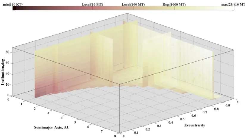
[image:7.595.90.502.396.628.2]trajectory can be computed. Fig. 5 shows the the maximum impact energy that can be deflected by the proposed kinetic deflector as a function of {a,e,i}.
Fig. 5. Deflected impact energy as a function of {a,e,i}.
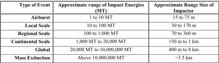
Finally, six different categories of impact hazard can be broadly defined by means of their impact energy (see Table 1) by following the approximate definitions proposed in [7]. Assuming spherical asteroids with average density (2600 g/m3 [8]), an approximate size range can also be estimated by considering the extreme variations of the impact velocity
of our set of impactors.
Table 1. Impact hazard categories
Type of Event Approximate range of Impact Energies (MT)
Approximate Range Size of Impactor
Airburst 1 to 10 MT 15 to 75 m
Local Scale 10 to 100 MT 30 to 170 m
Regional Scale 100 to 1,000 MT 70 to 360 m
Continental Scale 1,000 MT to 20,000 MT 150 m to 1 km
Global 20,000 MT to 10,000,000 MT 400 m to 8 km
Mass Extinction Above 10,000,000 MT >3.5 km
An estimate on the level of protection that the kinetic impactor presented here could be capable of providing can be calculated by summing up the relative impact frequency of each virtual impactor that can be deflected up to a given level of energy. For example, from the data represented in Fig. 5, it can be seen that the region with maximum impact energy deflected bellow 10 MT accounts for 2.6 % of the impacts, thus it can be suggested that the kinetic impactor could potentially deflect 97.4% of any incoming impact threat within the range defined as Airburst event. In the same way, the 1,000 kg kinetic impactor offers a 65.4% of protection against Local Scale events and 11.2% against Regional Scale. On the other hand, such a small impactor could not offer any realistic protection against any higher energy impacts.
CONCLUSIONS
This paper estimated the level of planetary protection that a 1,000 kg kinetic impactor could provide with a 20 year warning time. Optimal intercepting trajectories were designed to deflect a set of 17,518 virtual impactors and from there the maximum mass that can be deflected was computed. By considering the relative impact frequency of each virtual impactor, the percentage of planetary protection for different impact hazard scales can be assessed. Mitigation missions with a 1,000 kg spacecraft could safely deflect 97.4% of the airburst scale impact hazard, 65.4% of local scale events and 11.2% among the regional scale hazards. Unfortunately, impact events with energies above 20,000 MT cannot be effectively deflected with a 1-tonne spacecraft. Nevertheless, the kinetic impactor analysed here can be considered to be a small mission, well within the current capabilities for interplanetary space systems, and thus the levels of planetary protection achieved are satisfactory. These levels of protection, of course, assume that the threatening objects are discovered in advance, allowing 20 years of warning time to accommodate the optimal transfer and deflection manoeuvre. This is perhaps an optimistic assumption for very small objects, and future work should account for the time that objects on given orbits would take to be discovered, and reduce the warning time accordingly.
REFERENCES
[1] Sanchez, J. P., Colombo, C., Vasile, M. and Radice, G., “Multi-Criteria Comparison among Several Mitigation Strategies for Dangerous near Earth Objects,” Journal of Guidance, Control and Dynamics, Vol. 32, No. 1, 2009, pp. 121-142. doi: 10.2514/1.36774
[2] Vasile, M. and Colombo, C., “Optimal Impact Strategies for Asteroid Deflection,” Journal of Guidance, Control, and Dynamics, Vol. 31, No. 4, 2008, pp. 858-872. doi: 10.2514/1.33432
[3] Bottke, W. F., Morbidelli, A., Jedicke, R., Petit, J.-M., Levison, H. F., Michel, P. and Metcalfe, T. S., “Debiased Orbital and Absolute Magnitude Distribution of the near-Earth Objects,” Icarus, Vol. 156, No. 2, 2002, pp. 399-433. doi: 10.1006/icar.2001.6788
[4] Opik, E. J., “Collision Probabilities with the Planets and the Distribution of Interplanetary Matter,”
Proceedings of the Royal Irish Academy. Section A: Mathematical and Physical Sciences, Vol. 54, 1951/1952, pp. 165-199
[5] Sanchez, J. P. and McInnes, C. R., “Asteroid Resource Map for near-Earth Space,” Journal of Spacecraft and Rockets, Vol. 48, No. 1, 2011, pp. 153-165. doi: 10.2514/1.49851
[6] Vasile, M., “A Behavioral-Based Meta-Heuristic for Robust Global Trajectory Optimization,” Proceedings of
the IEEE Congress on Evolutionary Computation (CEC 2007), Inst. of Electrical and Electronics Engineers,
Piscataway,NJ, 25–28 Sept. 2007, pp. pp. 2056–2063.
[7] Shapiro, I. I. and al., e., “Defending Planet Earth: Near-Earth Object Surveys and Hazard Mitigation Strategies,” National Research Council, 2010.