(will be inserted by the editor)
Preconditioning for radial basis function partition of unity
methods
Alfa Heryudono · Elisabeth Larsson · Alison Ramage · Lina von Sydow
Received: date / Accepted: date
Abstract Meshfree radial basis function (RBF) methods are of interest for solving
par-tial differenpar-tial equations due to attractive convergence properties, flexibility with respect to geometry, and ease of implementation. For global RBF methods, the computational cost grows rapidly with dimension and problem size, so localised approaches, such as partition of unity or stencil based RBF methods, are currently being developed. An RBF partition of unity method (RBF–PUM) approximates functions through a combination of local RBF approximations. The linear systems that arise are locally unstructured, but with a global structure due to the partitioning of the domain. Due to the sparsity of the matrices, for large scale problems, iterative solution methods are needed both for computational reasons and to reduce memory requirements. In this paper we implement and test different algebraic pre-conditioning strategies based on the structure of the matrix in combination with incomplete factorisations. We compare their performance for different orderings and problem settings and find that a no-fill incomplete factorisation of the central band of the original discretisa-tion matrix provides a robust and efficient precondidiscretisa-tioner.
Authors are listed in alphabetical order.
Heryudono was partially supported by AFOSR grant FA9550-09-1-0208 and by National Science Foundation grant DMS-1318427.
A. Heryudono
Department of Mathematics, University of Massachusetts, Dartmouth, Massachusetts, 02747, USA Tel.: +1-508-999-8516
E-mail: [email protected]
E. Larsson
Department of Information Technology, Uppsala University, Box 337, 751 05 Uppsala, Sweden Tel.: + 46-18-471 2768
E-mail: [email protected]
A. Ramage
Department of Mathematics and Statistics, University of Strathclyde, Glasgow, G1 1XH, Scotland Tel.: +44-141-548 3801
E-mail: [email protected]
L. von Sydow
Department of Information Technology, Uppsala University, Box 337, 751 05 Uppsala, Sweden Tel.: + 46-18-471 2785
Keywords radial basis function·partition of unity·RBF–PUM·iterative method ·
preconditioning·algebraic preconditioner
Mathematics Subject Classification (2000) MSC 65F08·MSC 65M70
1 Introduction
There is an increasing interest in using methods based on radial basis function (RBF) ap-proximation [12] for the solution of partial differential equations (PDEs). The main advan-tages of these methods are that they are mesh free, which provides flexibility with respect to the geometry of the computational domain; they can be spectrally accurate for smooth solution functions [30, 31]; they are comparatively easy to apply to high-dimensional prob-lems, which is vital for application areas such as finance, quantum dynamics, and systems biology.
The typical form of an RBF approximation ˆu(x)to a solution function u(x), where x= (x1, . . .,xd)∈Rd, is
ˆ u(x) =
N
∑
j=1λjφj(x), (1)
whereλjare coefficients to be determined. Hereφ(r)is a radial basis function, andφj(x) =
φ(εkx−xjk), where xj, j=1, . . . ,N are the (scattered) node points at which the individual RBFs are centred. The parameterεis called the shape parameter and controls the flatness of the RBFs. This shape parameter has a significant influence on the accuracy of the approxi-mation, as well as on the conditioning of the resulting linear systems.
By requiring the RBF approximation to interpolate the solution at the node points, we arrive at a linear system
Aλ=u, (2)
many different types of methods, including RBF methods, were evaluated for option pricing problems. The results demonstrated that out of the implemented RBF methods, the RBF– PUM approach was the most efficient computationally.
The RBF–PUM discretisation leads to sparse unstructured matrices. For larger problem sizes and in higher dimensions, it is therefore necessary in terms of computational efficiency to use an iterative solver for the linear systems that arise. Here we use the Krylov subspace method GMRES [33] in order to take advantage of its theoretical residual minimising prop-erty (see§4): other methods such as Bi-CGSTAB [40] or IDR [38] may be more suitable for practical implementation with large problems. The RBF-PUM matrices are non-symmetric and moderately ill-conditioned so iterative convergence is typically very slow. It is therefore important to have an effective preconditioner for these systems. In this paper, we design and evaluate the performance of algebraic preconditioners based on (incomplete) LU factorisa-tion that take advantage of the underlying structure of the coefficient matrices. To the best of our knowledge, this is the first time that any preconditioner for this type of discretisation has been developed.
In the current literature, most papers on preconditioning for RBF interpolation or ap-proximation consider global apap-proximations like (1). In such circumstances, using precon-ditioners based on approximate cardinal basis functions computed on a reduced node set has been shown to be successful (see, e.g., [4, 6, 13, 20, 27]). In our case, we are using a lo-cal approximation, so the coefficient matrices are already sparse. Preconditioners utilising the Toeplitz structure of a discretisation with a logically Cartesian node layout are intro-duced in [3, 7]. Although efficient, these may be hard to use for the unstructured sets of nodes which are useful for non-trivial geometries. In [11], algebraic preconditioners are constructed for compactly-supported RBFs, utilising the two-by-two block structure of the matrix arising from the separation of boundary and interior nodes, in combination with an additive Schwarz method. A similar type of algebraic preconditioner is investigated in [1], for a special case of complex matrices with symmetric positive definite real and imaginary parts. In the latter paper, sparsification is used for the RBF example, in the sense that small off-diagonal elements are removed, and their mass is added to the corresponding diagonal element.
The remainder of this paper is structured as follows. In§2, we present details of the RBF discretisation method. This is followed in§3 by a description of the set of Poisson test problems which we use throughout the paper, together with a discussion of some important issues concerning node numbering and matrix structure. In §4, the iterative method and new preconditioners are described, and in§5 we make some predictions concerning the asymptotic convergence rates of the resulting methods. Finally, in§6, we present the results of several numerical experiments and draw some conclusions in§7.
2 The Radial Basis Function Partition of Unity Method
Since in this paper we are mainly interested in the efficiency of different preconditioning approaches, we restrict our attention to a stationary linear PDE with Dirichlet boundary conditions. We note, however, that the techniques presented here can also be generalised to other problem settings, including time-dependent problems. We define our model PDE on a closed domainΩ⊂Rd, with boundary∂Ωas follows:
Lu(x) =f(x), inΩ, (3a)
where x= (x1, . . . ,xd). In the numerical experiments presented later, we takeL =−∆(the Laplace operator).
In a partition of unity method, the global approximation ˜u(x)to the solution u(x)is constructed as a weighted sum of local solutions ˜uj(x)on overlapping patches Ωj, j= 1, . . . ,P. That is,
˜ u(x) =
P
∑
j=1wj(x)u˜j(x). (4)
where wj, j=1, . . . ,P are weight functions. The patchesΩjneed to form a cover of the domain in the sense that
P [
j=1
Ωj⊇Ω.
There should also be an upper bound K for the number of patches that overlap at one given point x∈Ω.
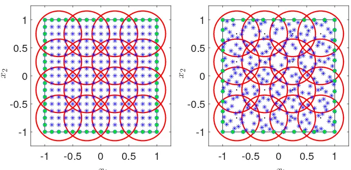
An illustration of typical sets of circular patches used in this paper can be seen in Fig-ure 1 in§3. We define the overlapγrelative to the minimal patch radius R0such that, for given patch centres, we fulfil the conditions required for a cover. That is, in subfigures 1(a) and 1(b), a patch radius of R0 would correspond to patch boundaries just touching in the diagonal direction. With an overlapγ, we use a patch radius of R= (1+γ)R0.
The partition of unity weight functions wjare non-negative, compactly supported onΩj and satisfy
P
∑
j=1wj(x) =1, ∀x∈Ω.
Furthermore, the weight functions need to be p times continuously differentiable, where p is the order of the PDE operatorL (forL =−∆, p=2). We follow the approach in [24, 34, 36], and use Shepard’s method [12, 37] applied to compactly supported C2 Wendland functions [41] to construct the weight functions
wj(x) = ϕ j(x)
∑P j=1ϕj(x)
, j=1, . . . ,P,
whereϕj(x)is the particular Wendland function supported onΩj.
The PDE (3) is discretised with a collocation method. We therefore define a global set of distinct nodes X={xk}Nk=1inΩ, requiring the PDE (3a) to be satisfied at interior nodes, and the boundary condition (3b) to be satisfied at boundary nodes. That is, we require
Lu˜(xk) = P
∑
j=1L(wj(xk)uj˜(xk)) =f(xk), xk∈Ω\∂Ω, (5a)
˜ u(xk) =
P
∑
j=1wj(xk)u˜j(xk) =g(xk), xk∈∂Ω. (5b)
For the particular case of the Poisson problem, whereL =−∆, the local operator can be expanded to give
L(wj(x
When using partition of unity approximations such as (5), it is convenient to work at the patch level. We therefore now define local subsets of nodes as Xj={xij}
nj
i=1={xk∈ X|xk∈Ωj}, where nj is the number of nodes that fall in Ωj. In addition, we define the index mapping k=π(i,j)that returns the global index k for a given local node xij. In the particular case of RBF-PUM, the local solutions ˜uj(x)are RBF approximations
˜ uj(x) =
nj
∑
i=1λj iφ
j
i(x), (7)
whereλijare coefficients to be determined andφij(x) =φ(εkx−xijk). However, in the par-tition of unity setting, it is inconvenient to use the coefficientsλijas the degrees of freedom, as there is more than one coefficient per collocation node in the regions of overlap between patches. Instead, we solve for the nodal values ˜uj(x
j
i)≡u˜(xk), where k=π(i,j). That is, we require the local solution from two adjacent patches to take on the same value at the node points in the overlap region. The same requirement expressed in terms of the coefficients would result in a non-local condition involving all coefficents in both patches.
We now define the vector of local nodal values uj= (u˜j(x1j), . . .,u˜j(xnjj))Tand the local coefficient vectorλj= (λ
j 1, . . . ,λ
j
nj)T. From (7), we then have the relations Ajλj=uj ⇒ λj=A−j1uj,
where Aj={φmj(xij)} nj
i,m=1, and
Luj=DLj λj=DLj A−1 j uj,
where DLj ={Lφ j m(xij)}
nj
i,m=1. Note that, for distinct node points with positive definite RBFs such as the Gaussians used for the numerical experiments in this paper, the local RBF interpolation matrices Ajare guaranteed to be non-singular [35]. We also define a diagonal matrix
WjL =diag(Lwj(x j
1), . . .,Lwj(xnjj))
associated with each patch. Now, using (6), we can express the discrete local Laplacian operators as
˜Lj= (Wj∆Aj+2Wj∇·D∇j +WjD∆j)A− 1 j ,
where the gradient operators are vector valued, and the scalar product is applied in the appro-priate way. To get the discrete local PDE operator, we also include the boundary conditions, which gives
Lj(i,m) = (
˜Lj(i,m),x j
i ∈Ω\∂Ω,
δim, x j i ∈∂Ω,
whereδimis the Kronecker delta. Finally, we obtain the global discrete operator by, as in a finite element method, assembling the local matrices Ljinto the global matrix L such that
Lj(i,m)−→+ L(π(i,j),π(m,j)), j=1, . . . ,P, i,m=1, . . . ,nj. The global right hand side f= (f1, . . .,fN)Tis defined through
fk=
With the global vector of nodal values defined by u= (x1, . . . ,xN)T, the final (global) linear system to be solved is
Lu= f. (8)
For small values of the shape parameterε, the matrices Lj, and consequently L, become highly ill-conditioned when computed as described above [18, 19]. This is problematic be-cause, for smooth solution functions, a small positive shape parameter value typically gives the best accuracy of the solution [17, 22, 23]. Furthermore, refining the patches in RBF-PUM for a fixedε results in a decreasing ’effective’ shape parameter value, that is, the shape parameter becomes smaller in relation to the patch size. However, the problem of ill-conditioning for small shape parameters can be avoided by employing stable evaluation methods such as the Contour-Pad´e approach [17], the RBF-QR method [14, 16, 25], or the RBF-GA method [15]. Here we employ the RBF-QR method which, simply put, corre-sponds to a change of basis from{φmj}to{ψmj} in the local problems. This significantly reduces the condition number of Aj, and allows for stable evaluation of Ljfor small shape parameter values.
3 Model problems and ordering issues
To fix ideas, we will focus for the remainder of the paper on two specific two-dimensional model problems. As stated above, we will solve the PDE (3) withL =−∆ (the Laplace operator). For simplicity, we use a manufactured solution u(x)from which we can compute the right-hand-side functions f and g, namely,
u(x) =sin(x21+2x22)−sin(2x21+ (x2−0.5)2). (9) We solve this problem over two different two-dimensional physical domainsΩ: for Model Problem I, the domain is the squareΩ= [−1,1]2, and for Model Problem II, the boundary ofΩ is defined by
∂Ω={(r,θ)|r(θ) =0.8+0.1(sin(6θ) +sin(3θ))}. (10)
This region is illustrated in Figure 1(c).
In Figure 1 we show typical examples of patches and node distributions for Model Prob-lem I (with 16 patches on the square domain) and Model ProbProb-lem II (with 50 patches and domain boundary defined by (10)). In each case, the patch boundaries are shown in red, with patch centres marked as black dots. Points on the domain boundary (where the Dirich-let boundary conditions are applied) are represented by green circles. The amount of overlap between patches isγ=0.15 for Model Problem I, andγ=0.3 for Model Problem II. The square domain is shown with both Cartesian and Halton [21] nodes (shown as blue stars). The reason for choosing these two types of nodes is that they represent extremes in terms of node distributions: the Cartesian nodes are completely structured, while the Halton nodes are quasi random, and completely unstructured. For general geometries it is not possible to always have completely structured nodes. A typical scenario for a RBF-PUM discretisation would be to have unstructured nodes, but of a higher quality in terms of uniformity than Halton nodes. This is the case that is investigated for Model Problem II, see Figure 1(c).
x1
-1 -0.5 0 0.5 1 x2
-1 -0.5 0 0.5 1
(a) Model Problem I, 289 Cartesian nodes, 16 patches.
x1
-1 -0.5 0 0.5 1 x2
-1 -0.5 0 0.5 1
(b) Model Problem I, 294 Halton nodes, 16 patches.
x1
-1 -0.5 0 0.5 1 x2
-1 -0.5 0 0.5 1
[image:7.612.77.422.44.211.2](c) Model Problem II, 298 unstructured nodes, 50 patches.
Fig. 1: Illustrations of typical patches and node distributions. Patch boundaries are marked with red circles, interior nodes with blue stars and boundary nodes with green circles.
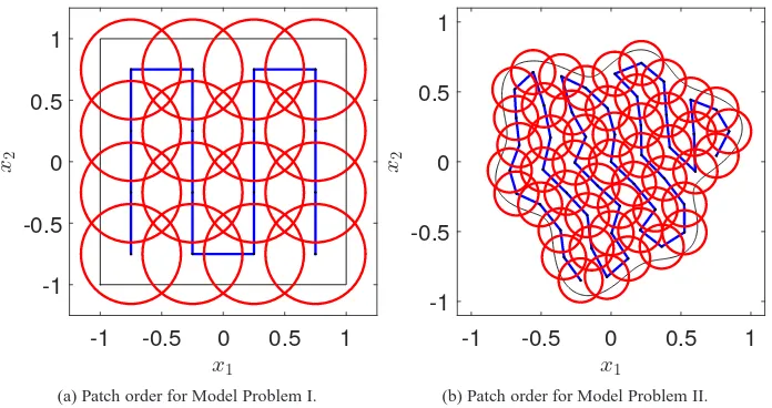
One question which needs addressing is how the patches, and then the nodes within each patch, should be ordered. This is important as the sparsity pattern of L in (8) will have implications for the design of efficient fast solvers. In particular, as we will consider sparse factorisation techniques, we are interested in keeping the matrix entries as tightly banded as possible. To this end, we choose a snake ordering for the patches, where each patch (except the last) is followed by one of its neighbours. This ordering is illustrated for both model problems in Figure 2, where the patch ordering follows the blue line.
ob-x1
-1 -0.5 0 0.5 1 x2
-1 -0.5 0 0.5 1
(a) Patch order for Model Problem I.
x1
-1 -0.5 0 0.5 1 x2
-1 -0.5 0 0.5 1
[image:8.612.75.423.46.230.2](b) Patch order for Model Problem II.
Fig. 2: Illustrations of the snake patch ordering strategy. The blue lines illustrate the order in which the patches are numbered.
vious how to proceed. We use the following simple heuristic approach. Starting with the patch whose centre has minimum y co-ordinate, we select a neighbour that is to the left or else above (in terms of the centre co-ordinates) for as long as possible. When this fails, we switch direction and look for a neighbour that is to the left or else below, continuing in this alternating way until all patches have been traversed. Although this approach may some-times fail (for example, when the domain has thin sections with only one layer of patches such that changing direction is not possible), the general principle of ordering patches in terms of nearest neighbours in a linear-like way should still be followed where possible.
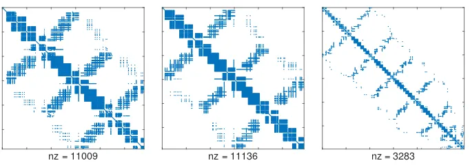
Having fixed an order for the patches, we now turn our attention to the ordering of nodes within each patch, with a similar aim of designing this to minimise the distance between neighbouring nodes. The strategy we use has two main components. First, each node xkis allocated to a home patch, according to its largest weight. That is, it is associated with the patchΩjfor which wj(xk)≥wi(xk), i=1, . . . ,P, see (4). In the case of a tie, the first patch with this property is designated the home patch. Secondly, the nodes are then ordered within each patch as follows: first, nodes in the overlap of the current and preceding patch; then nodes only in the current patch; finally, nodes in the overlap of the current and the following patch. In this way, nodes that are located in the overlap regions between patches become close neighbours in the ordering, leading to a cleaner structure in the final global matrix. Examples of the sparsity of L resulting from this patch and node ordering are shown in Figure 3, where the three subfigures correspond to the three model problem configurations presented in Figure 1.
4 Iterative method and preconditioning
nz = 11009
(a) Sparsity of L corresponding to patches and nodes in Figure 1(a).
nz = 11136
(b) Sparsity of L corresponding to patches and nodes in Figure 1(b).
nz = 3283
[image:9.612.75.416.34.154.2](c) Sparsity of L corresponding to patches and nodes in Figure 1(c).
Fig. 3: Illustrations of typical sparsity patterns of L corresponding to the sample patch and node combinations in Figure 1.
memory requirements, especially for high-dimensional PDE problems. Instead, we adopt an iterative approach to take full advantage of the sparsity induced by the local approximation. In this paper, we will focus on the Generalized Minimum Residual (GMRES) method [33]. As mentioned in the introduction, GMRES is usually not the most efficient method in prac-tice, as it involves storing and re-orthogonalising against an increasing number of vectors at each iteration. For implementation purposes, the restarted version GMRES(m) should be used, or an alternative more cost effective Krylov method such as Bi-CGSTAB [40] or IDR [38]. However, we use GMRES here for its clear theoretical framework as outlined below.
It is well known that the convergence of GMRES (and other iterative methods) can be improved by introducing the concept of preconditioning. Theoretically, this is equivalent to replacing L by a preconditioned matrix whose eigenvalue spectrum facilitates faster itera-tive convergence(see below). Considerable research has been carried out in recent years to find inexpensive ways to generate suitable preconditioners for a wide variety of problems with different types of coefficient matrix (see, for example, [5] or any standard textbook on iterative methods). Here we will employ right preconditioning and solve linear systems equivalent to (8) of the form
LM−1y=f, Mu=y.
Note that in practice it is not necessary to form the preconditioned matrix LM−1explicitly (which would again result in a loss of sparsity): we only need to solve ‘inner’ linear systems with M as coefficient matrix. The aim is therefore to find a preconditioner M such that LM−1 has an improved eigenvalue structure, while a system with coefficient matrix M is cheap to solve. This latter point is primarily what motivates the use of sparse factorisations as preconditioners.
The GMRES method has the attractive theoretical property of minimising the 2-norm of the residual at each iteration. That is, at iteration i, the residual vector ri= f−LM−1yi satisfies
krik2= min
pi∈Pi,pi(0)=1kpi(LM −1
wherePiis the set of all polynomials of degree i. Furthermore, if the preconditioned coef-ficient matrix LM−1is diagonalisable, it can be shown that
krik2
kr0k 2
≤cond2(WLM−1) min
pi∈Pi,pi(0)=11max≤ℓ≤N|pi(αℓ)|
whereαℓ,ℓ=1, . . . ,N are the eigenvalues of LM−1with corresponding eigenvector matrix WLM−1.If LM−1 is normal, then cond2(WLM−1) =1 and,in exact arithmetic, GMRES will converge in s iterations, where s is the number of distinct eigenvalues of LM−1. In prac-tice, although rounding error pollutes this theoretical result, the rate of convergence is still essentially bounded by the quantity
ρi= min
pi∈Pi,pi(0)=11max≤ℓ≤N|pi(αℓ)| (11) at each iteration, so fast convergence can be obtained if the eigenvalues of LM−1are nicely clustered. Specifically, if the preconditioned eigenvalues lie in k dense clusters, we expect to obtain a good approximation to the solution vector in k GMRES iterations.If the precondi-tioned coefficient matrix is not normal (as is the case here), the factor cond2(WLM−1)reflects its degree of non-normality and convergence often exhibits an initial period of stagnation be-fore bounds based on eigenvalues alone become descriptive [10]. This phenomenon can be observed in the convergence plots presented later (Figure7).
In the numerical experiments in§6, we will compare the performance of five different preconditioners with that of unpreconditioned GMRES. Two of these are based on a straight-forward incomplete LU factorisation [29] of L. In the first (L-ILUn), no fill-in is allowed, that is, the sparsity pattern of the factors is fixed to the same as the sparsity pattern of the original matrix L (this method is often designated in the literature by ILU(0)). In the second variant (L-ILUd), a drop tolerance is specified (0.001 in our experiments), and any poten-tial entries in the factors which are less than this value are ignored, again ensuring that the factors remain sparse.
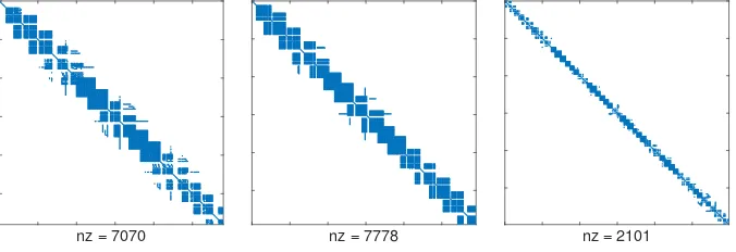
In addition to these two standard methods, we will also use three preconditioners based on factorisations of an alternative matrix, B, containing only the central band of L. Figure 4 shows the matrix B for the three configurations we have considered in Figures 1 and 3. In
nz = 7070
(a) Sparsity of B corresponding to patches and nodes in Figure 1(a).
nz = 7778
(b) Sparsity of B corresponding to patches and nodes in Figure 1(b).
nz = 2101
[image:10.612.77.415.430.546.2](c) Sparsity of B corresponding to patches and nodes in Figure 1(c).
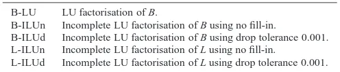
each case, the bandwidthβ of B (such that bi j =0 when|i−j|>β) has been set equal to maxjnj−1 where njis the total number of nodes in patch j. This choice of bandwidth ensures that we retain information about the closest connections between nodes and patches, which is located in this central band thanks to the nearest-neighbour philosophy we have used in numbering of patches and nodes (see§3). In§6, we test three preconditioners based on B. The first of these is a full LU factorisation of B (B-LU). Although this will not be competitive in computational terms, the resulting iteration counts will give an indication of the amount of information lost by replacing the full coefficient matrix L with the banded approximation B. As more practical preconditioners, we also use the same two forms of ILU factorisation used for L, namely, with no fill-in (B-ILUn) and with a drop tolerance of 0.001 (B-ILUd). A summary of all five preconditioners implemented in§6, together with the acronyms used to refer to them in the following text, is given in Table 1.
Table 1: Summary of preconditioners implemented
B-LU LU factorisation of B.
B-ILUn Incomplete LU factorisation of B using no fill-in.
B-ILUd Incomplete LU factorisation of B using drop tolerance 0.001. L-ILUn Incomplete LU factorisation of L using no fill-in.
L-ILUd Incomplete LU factorisation of L using drop tolerance 0.001.
Note that, in terms of ILU fixed sparsity patterns, we have included here results only for the no-fill version (commonly called ILU(0)) and not the more general version, ILU(p) (see, for example, [32,§10.3.3]) which allows a higher level of fill-in. For the banded fac-torisation, we observed in our numerical experiments that most of the relevant information is already captured by B-ILUn, making versions with more fill-in essentially redundant. For the full factorisation of L, adding additional fill-in was more beneficial in terms of reducing iteration counts. However, the amount of extra storage required grew very quickly, making such methods unattractive when moving to high dimensional problems. We have therefore omitted results obtained using these methods from this paper.
5 Convergence estimates for GMRES
As described in §4, the asymptotic convergence phase of GMRES can be quantified by considering the factorsρiin (11) based on the eigenvaluesαℓof the coefficient matrix. In practice, however, the eigenvaluesαℓ are not usually readily available, so it is common to use instead a related expression, based on a compact and continuous set S which contains the relevant eigenspectrum (but excludes the origin), of the form
ρi(S) = min
pi∈Pi,pi(0)=1maxσ∈S|pi(σ)|.
To remove the dependence on the iteration number i, it is often more convenient to consider the so-called asymptotic convergence factor of the set S (see e.g. [26,§5.7.6]) defined by
ρ(S) =lim i→∞(ρi(S))
1/i
Althoughρ(S)can be difficult to quantify analytically, its value can be estimated using a computational technique based on conformal mappings. Specifically, ifΦ is a conformal map from the exterior of S to the exterior of the unit disc that satisfiesΦ(∞) =∞, thenρ(S)
in (12) can be approximated by the value of|Φ(0)|−1 (see [9] for more details). In what follows, we apply this technique with S chosen to be the complex hull of the eigenvalue spectrum being studied.
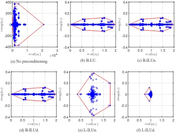
We begin with Model Problem I with Cartesian grid points, but here using more points (N=1225, with 64 (8×8) patches) than shown in Figure 1(a). Gaussian RBFs,φ(εr) =
exp(−ε2r2), with shape parameterε=1.2 are used. Here L (and its associated precondi-tioned versions) is positive definite, so the convex hull of the eigenvalues does not contain the origin, and the procedure for estimating the asymptotic convergence factor outlined above can be carried out in all cases. The pictures in Figure 5 show the eigenvalues (blue circles) of the coefficient matrix after the different preconditioners have been applied, with the convex hull outlined in red.
real(αℓ) ×104
0 1 2 3
ima g ( αℓ ) -400 -200 0 200 400
(a) No preconditioning.
real(αℓ)
0 0.5 1 1.5 2
ima g ( α ℓ ) -0.4 -0.2 0 0.2 0.4 (b) B-LU.
real(αℓ)
0 0.5 1 1.5 2
ima g ( α ℓ ) -0.4 -0.2 0 0.2 0.4 (c) B-ILUn.
real(αℓ)
0 0.5 1 1.5 2
ima g ( α ℓ ) -0.4 -0.2 0 0.2 0.4 (d) B-ILUd.
real(αℓ)
0 0.5 1 1.5 2
ima g ( α ℓ ) -0.4 -0.2 0 0.2 0.4 (e) L-ILUn.
real(αℓ)
0 0.5 1 1.5 2
[image:12.612.72.422.229.494.2]ima g ( α ℓ ) -0.4 -0.2 0 0.2 0.4 (f) L-ILUd.
Fig. 5: Eigenvalues of the coefficient matrix with various preconditioners for Model Problem I with 1225 Cartesian points and 64 patches together with the associated convex hull used in the calculation ofρin (12).
Table 2: Approximate asymptotic convergence factor for Model Problem I with 1225 Cartesian points and 64 patches using different preconditioners.
None B-LU B-ILUn B-ILUd L-ILUn L-ILUd
0.990 0.839 0.839 0.840 0.506 0.132
the same convergence factor. An improvement in GMRES convergence rate is anticipated with all three. The fact that the two preconditioners based on L lead to very clustered eigen-values (Figures 5(e) and (f)) is reflected in the much smaller eigen-values ofρpredicted for these methods, suggesting that they will require few iterations for convergence.
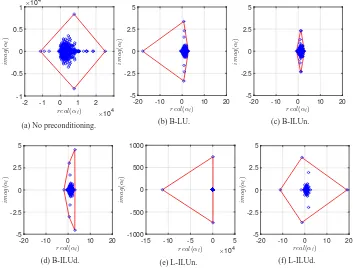
Analogous eigenvalue plots for Model Problem I with 1258 Halton points and 64 patches are shown in Figure 6. Here, the convex hull of the eigenvalues always contains the origin
real(αℓ) ×104
-2 -1 0 1 2
ima
g
(
αℓ
)
×104
-1 -0.5 0 0.5 1
(a) No preconditioning.
real(αℓ)
-20 -10 0 10 20
ima g ( α ℓ ) -5 -2.5 0 2.5 5 (b) B-LU.
real(αℓ)
-20 -10 0 10 20
ima g ( α ℓ ) -5 -2.5 0 2.5 5 (c) B-ILUn.
real(αℓ)
-20 -10 0 10 20
ima g ( α ℓ ) -5 -2.5 0 2.5 5 (d) B-ILUd.
real(αℓ) ×104
-15 -10 -5 0 5
ima g ( αℓ ) -1000 -500 0 500 1000 (e) L-ILUn.
real(αℓ)
-20 -10 0 10 20
[image:13.612.70.423.234.505.2]ima g ( α ℓ ) -5 -2.5 0 2.5 5 (f) L-ILUd.
Fig. 6: Eigenvalues of the coefficient matrix with various preconditioners for Model Problem I with 1258 Halton points and 64 patches together with the associated convex hull. Note that the axis limits are the same for all preconditioned spectra except for the L-ILUn preconditioner.
iterations (k)
0 50 100 150 200 250
lo
g10
(
k
rk
k2
/
k
r0
k2
)
10-8 10-6 10-4 10-2 100
none B-LU B-ILUn B-ILUd L-ILUn L-ILUd
(a) 1225 Cartesian points.
iterations (k)
0 100 200 300 400 500
lo
g10
(
k
rk
k2
/
k
r0
k2
)
10-8 10-6 10-4 10-2 100
none B-LU B-ILUn B-ILUd L-ILUn L-ILUd
[image:14.612.73.419.49.226.2](b) 1258 Halton points.
Fig. 7: Convergence for Model Problem I using 64 patches.
starting guess, and each GMRES iteration was terminated when
krik2≤10−8kr0k2. (13) These results can be used to compute the residual reduction factor ˜ρ, defined by
˜
ρ=
krik2
kr0k 2
1/i
,
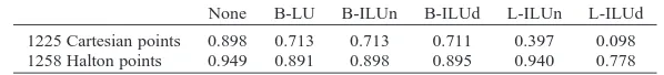
where i is the number of iterations required for convergence. These values are shown in Table 3. The actual residual reduction factor for the Cartesian points is slightly better than expected from theory (Table 2) but exhibits the same relative behaviour over the range of preconditioners.
Table 3: Residual reduction for Model Problem I with 64 patches and 1225 Cartesian points and 1258 Halton points respectively, using different preconditioners.
None B-LU B-ILUn B-ILUd L-ILUn L-ILUd
1225 Cartesian points 0.898 0.713 0.713 0.711 0.397 0.098 1258 Halton points 0.949 0.891 0.898 0.895 0.940 0.778
6 Numerical results
[image:14.612.94.393.459.493.2]usingticandtoc. The initial guess was zero, and all tests used the GMRES stopping cri-terion (13). The underlying PDE problems which we solve are Model Problems I and II as described in§3. However, as we are interested in studying the effect on solver performance of varying the number of patches, as well as the type and number of points used, we do not limit ourselves to the configurations shown in Figure 1. Instead we will introduce five sets of test problems which will help us to isolate these individual effects. In all experiments, Gaussian RBFs with shape parameterε=1.2 have been used. The RBF–QR method was employed in order to ensure stable evaluation of the matrices. It should however be noted that even if the RBF–QR method involves a change of basis, the resulting differentiation matrices are the same that would result from a direct use of the Gaussian basis if that was numerically feasible.
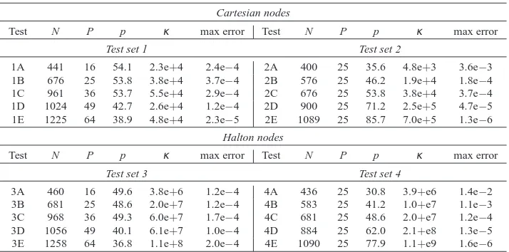
[image:15.612.72.429.257.434.2]The first four of these test sets are for Model Problem I (on the square domain). For each test problem, the number of points (N), number of patches (P), average number of of points per patch (p), estimated condition number of L (κ, calculated using the MATLAB command condest), and the maximum error in the discrete solution are displayed in Table 4. Test sets
Table 4: Test sets 1–4 for Model Problem I
Cartesian nodes
Test N P p κ max error Test N P p κ max error
Test set 1 Test set 2
1A 441 16 54.1 2.3e+4 2.4e−4 2A 400 25 35.6 4.8e+3 3.6e−3 1B 676 25 53.8 3.8e+4 3.7e−4 2B 576 25 46.2 1.9e+4 1.8e−4 1C 961 36 53.7 5.5e+4 2.9e−4 2C 676 25 53.8 3.8e+4 3.7e−4 1D 1024 49 42.7 2.6e+4 1.2e−4 2D 900 25 71.2 2.5e+5 4.7e−5 1E 1225 64 38.9 4.8e+4 2.3e−5 2E 1089 25 85.7 7.0e+5 1.3e−6
Halton nodes
Test N P p κ max error Test N P p κ max error
Test set 3 Test set 4
3A 460 16 49.6 3.8e+6 1.2e−4 4A 436 25 30.8 3.9+e6 1.4e−2 3B 681 25 48.6 2.0e+7 1.2e−4 4B 583 25 41.2 1.0+e7 1.1e−3 3C 968 36 49.3 6.0e+7 1.7e−4 4C 681 25 48.6 2.0+e7 1.2e−4 3D 1056 49 40.1 6.1e+7 1.0e−4 4D 884 25 62.0 2.1+e8 1.3e−5 3E 1258 64 36.8 1.1e+8 2.0e−4 4E 1090 25 77.9 1.1+e9 1.6e−6
1 and 2 both use Cartesian points. In test set 1, N and P are both increased in such a way that the resulting error in the solution is kept at a similar level (≃1e−4). This results in a set of coefficient matrices L which are similarly conditioned. Note that problem 1E corresponds to the configuration which leads to the eigenvalues in Figure 5. Test set 2 is designed to achieve different levels of accuracy by varying N while keeping P constant (P=25). Here it is clear that there is a correlation between the accuracy of the discretisation and the condition of the resulting L. Test sets 3 and 4 are designed to be broadly similar, but use Halton points in place of a Cartesian lattice. The degradation of the condition number of L associated with the irregularly scattered points is apparent.
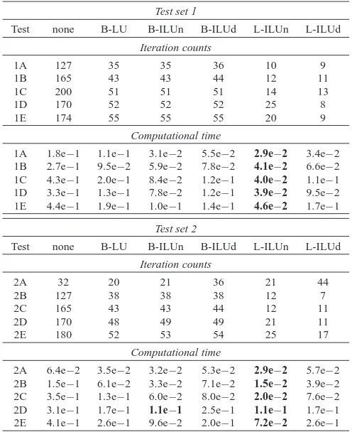
Table 5: Results for test sets 1 and 2 (Cartesian nodes, Model problem I). The lowest time for each problem is shown in bold.
Test set 1
Test none B-LU B-ILUn B-ILUd L-ILUn L-ILUd
Iteration counts
1A 127 35 35 36 10 9
1B 165 43 43 44 12 11
1C 200 51 51 51 14 13
1D 170 52 52 52 25 8
1E 174 55 55 55 20 9
Computational time
1A 1.8e−1 1.1e−1 3.1e−2 5.5e−2 2.9e−2 3.4e−2 1B 2.7e−1 9.5e−2 5.9e−2 7.8e−2 4.1e−2 6.6e−2 1C 4.3e−1 2.0e−1 8.4e−2 1.2e−1 4.0e−2 1.1e−1 1D 3.3e−1 1.3e−1 7.8e−2 1.2e−1 3.9e−2 9.5e−2 1E 4.4e−1 1.9e−1 1.0e−1 1.4e−1 4.6e−2 1.7e−1
Test set 2
Test none B-LU B-ILUn B-ILUd L-ILUn L-ILUd
Iteration counts
2A 32 20 21 36 21 44
2B 127 38 38 38 12 7
2C 165 43 43 44 12 11
2D 170 48 49 49 21 11
2E 180 52 53 54 25 17
Computational time
2A 6.4e−2 3.5e−2 3.2e−2 5.3e−2 2.9e−2 5.7e−2 2B 1.5e−1 6.1e−2 3.3e−2 7.1e−2 1.5e−2 3.9e−2 2C 3.5e−1 1.3e−1 6.0e−2 8.0e−2 2.0e−2 7.6e−2 2D 3.1e−1 1.7e−1 1.1e−1 2.5e−1 1.1e−1 1.7e−1 2E 4.1e−1 2.6e−1 9.6e−2 2.0e−1 7.2e−2 2.6e−1
using problem 1E), the method which converges in the smallest number of iterations is L-ILUd, followed by L-ILUn, while the three methods based on B have similar performance. As B-LU uses a full LU factorisation, iteration counts for this preconditioner give a lower bound on what can be expected from B-ILUn and B-ILUd. It can be seen that, as we have carefully numbered patches and points to ensure that the central band that is used to form B is relatively dense, very little is lost in replacing LU by an incomplete version. As well as considering iteration counts, however, it is of course important to consider the computational time taken by each method. Those are also listed in Table 5, and include the time taken for factorisation (where applicable) and the full GMRES solve. Using this measure, the methods of choice are the factorisations based on ILUn with, for these Cartesian examples, L-ILUn being slightly faster that the banded version, B-ILUn.
Table 6: Results for test sets 3 and 4 (Halton nodes, Model Problem I). The lowest time for each problem is shown in bold.
Test set 3
Test none B-LU B-ILUn B-ILUd L-ILUn L-ILUd
Iteration counts
3A 156 52 58 54 97 19
3B 231 100 112 106 167 49
3C 297 114 135 123 159 65
3D 310 108 118 115 202 60
3E 355 161 174 166 310 75
Computational time
3A 2.5e−1 1.0e−1 5.4e−2 1.9e−1 2.2e−1 1.7e−1 3B 5.5e−1 3.0e−1 1.6e−1 2.6e−1 3.1e−1 4.3e−1 3C 8.6e−1 3.9e−1 3.1e−1 4.1e−1 3.4e−1 8.5e−1 3D 9.5e−1 3.4e−1 2.1e−1 3.5e−1 6.3e−1 7.9e−1 3E 1.4e−0 6.3e−1 4.2e−1 6.2e−1 1.1e−0 1.1e−0
Test set 4
Test none B-LU B-ILUn B-ILUd L-ILUn L-ILUd
Iteration counts
4A 189 72 72 72 79 16
4B 209 80 91 84 147 34
4C 231 100 112 106 167 49
4D 262 107 125 124 176 66
4E 295 120 135 172 368 152
Computational time
4A 3.1e−1 1.1e−1 1.0e−1 1.8e−1 1.6e−1 1.6e−1 4B 4.6e−1 2.7e−1 1.9e−1 2.5e−1 2.4e−1 2.3e−1 4C 4.9e−1 3.0e−1 1.8e−1 3.0e−1 4.2e−1 3.9e−1 4D 6.5e−1 5.2e−1 2.8e−1 4.2e−1 4.1e−1 8.8e−1 4E 9.0e−1 6.9e−1 3.0e−1 8.8e−1 1.6e−0 2.8e−0
comes at the price of significantly increasing the amount of memory needed. The compara-tive merits of other methods in Table 6 are essentially the same as for the Cartesian example, although the reduction in iteration counts (relative to the unpreconditioned case) is less in all cases here. This is not surprising as the Halton points do not have the rigid banded substruc-ture of the Cartesian points, which is more amenable to efficient factorisation. In addition, the bandwidth measureβ in B has been tailored to the Cartesian case (where it can be eas-ily calculated): using the same measure in the Halton case does not necessareas-ily guarantee inclusion of all closest connections due to the lack of structure. However, the factorisations based on B still work well as preconditioners and, in terms of computational times, B-ILUn is clearly the most efficient method overall.
Table 7: Test set 5 for Model Problem II
Test N P p κ max error
5A 398 50 13.2 1.6e+6 8.8e−1 5B 695 50 23.4 9.7e+5 2.8e−4 5C 994 50 33.4 1.9e+7 2.2e−4 5D 1094 50 36.9 8.6e+6 8.4e−6 5E 1292 50 43.7 1.6e+7 1.7e−6
Table 8: Results for test set 5 (Model Problem II). The lowest time for each problem is shown in bold.
Test none B-LU B-ILUn B-ILUd L-ILUn L-ILUd
Iteration counts
5A 207 67 68 67 48 14
5B 235 76 78 76 85 13
5C 279 99 119 99 195 23
5D 304 102 120 102 255 26
5E 322 133 149 132 415 53
Computational time
5A 2.1e−1 7.3e−2 5.8e−2 7.3e−2 3.9e−2 3.0e−2
5B 4.9e−1 1.3e−1 8.8e−2 1.3e−1 9.9e−2 8.4e−2
5C 7.5e−1 2.6e−1 2.1e−1 2.6e−1 4.4e−1 2.8e−1 5D 9.1e−1 2.9e−1 2.1e−1 2.9e−1 7.4e−1 3.7e−1 5E 1.1e−0 5.6e−1 3.3e−1 5.3e−1 2.0e−0 7.9e−1
7 Conclusions
In this paper, we have introduced and evaluated algebraic preconditioners for RBF-PUM discretisations. These preconditioners are free of any assumptions on the node layout or geometry of the computational domain. The only property that is used is the knowledge that there is a patch structure and that nodes can be ordered accordingly. This is important so that the preconditioner is generally applicable.
The performance of the preconditioners, as well as the conditioning of the original ma-trix, is negatively affected by the use of the highly unstructured nodes. However, in our experiments we do not observe any adverse effect of changing the computational domain. The preconditioner that performed best overall, and that we recommend for use, is the no fill-in incomplete factorisation of the central band, denoted by B-ILUn.
The B-ILUn preconditioner is also the most sparse of the tested preconditioners. This property becomes increasingly important when moving to larger matrix sizes and/or higher dimensional problems, in which case memory requirements become a limiting factor. How the preconditioner performs in higher dimensions will be the subject of further studies.
References
1. Axelsson, O., Neytcheva, M., Ahmad, B.: A comparison of iterative methods to solve complex valued linear algebraic systems. Numer. Algorithms 66(4), 811–841 (2014). DOI 10.1007/s11075-013-9764-1 2. Babuˇska, I., Melenk, J.M.: The partition of unity method. Internat. J. Numer. Methods Engrg. 40(4),
[image:18.612.121.370.167.304.2]3. Baxter, B.J.C.: Preconditioned conjugate gradients, radial basis functions, and Toeplitz matrices. Com-put. Math. Appl. 43(3-5), 305–318 (2002). DOI 10.1016/S0898-1221(01)00288-7
4. Beatson, R.K., Cherrie, J.B., Mouat, C.T.: Fast fitting of radial basis functions: methods based on preconditioned GMRES iteration. Adv. Comput. Math. 11(2-3), 253–270 (1999). DOI 10.1023/A:1018932227617
5. Benzi, M.: Preconditioning techniques for large linear systems: A survey. J. Comp. Phys. 182, 418–477 (2002). DOI 10.1006/jcph.2002.7176
6. Brown, D., Ling, L., Kansa, E., Levesley, J.: On approximate cardinal preconditioning methods for solving PDEs with radial basis functions. Eng. Anal. Bound. Elem. 29(4), 343–353 (2005). DOI http://dx.doi.org/10.1016/j.enganabound.2004.05.006
7. Cavoretto, R., De Rossi, A., Donatelli, M., Serra-Capizzano, S.: Spectral analysis and preconditioning techniques for radial basis function collocation matrices. Numer. Linear Algebra Appl. 19(1), 31–52 (2012). DOI 10.1002/nla.774
8. Driscoll, T.A., Fornberg, B.: Interpolation in the limit of increasingly flat radial basis functions. Comput. Math. Appl. 43(3–5), 413–422 (2002). DOI 10.1016/S0898-1221(01)00295-4
9. Driscoll, T.A., Toh, K.C., Trefethen, L.N.: From potential theory to matrix iterations in six steps. SIAM Review 40, 547–578 (1998). DOI 10.1137/S0036144596305582
10. Embree, M.: How descriptive are gmres convergence bounds? Tech. Rep. 99/08, Oxford University Computing Laboratory Numerical Analysis (1999)
11. Farrell, P., Pestana, J.: Block preconditioners for linear systems arising from multilevel RBF collocation. MIMS EPrint 2014.18, Manchester Institute for Mathematical Sciences, School of Mathematics, The University of Manchester (2014)
12. Fasshauer, G.E.: Meshfree approximation methods with MATLAB, Interdisciplinary Mathematical
Sci-ences, vol. 6. World Scientific Publishing Co. Pte. Ltd., Hackensack, NJ (2007). DOI 10.1142/6437
13. Faul, A.C., Goodsell, G., Powell, M.J.D.: A Krylov subspace algorithm for multiquadric interpolation in many dimensions. IMA J. Numer. Anal. 25(1), 1–24 (2005). DOI 10.1093/imanum/drh021
14. Fornberg, B., Larsson, E., Flyer, N.: Stable computations with Gaussian radial basis functions. SIAM J. Sci. Comput. 33(2), 869–892 (2011). DOI 10.1137/09076756X
15. Fornberg, B., Lehto, E., Powell, C.: Stable calculation of Gaussian-based RBF-FD stencils. Comput. Math. Appl. 65(4), 627–637 (2013). DOI 10.1016/j.camwa.2012.11.006
16. Fornberg, B., Piret, C.: A stable algorithm for flat radial basis functions on a sphere. SIAM J. Sci. Comput. 30(1), 60–80 (2007). DOI 10.1137/060671991
17. Fornberg, B., Wright, G.: Stable computation of multiquadric interpolants for all values of the shape parameter. Comput. Math. Appl. 48(5-6), 853–867 (2004). DOI 10.1016/j.camwa.2003.08.010 18. Fornberg, B., Wright, G., Larsson, E.: Some observations regarding interpolants in the limit of flat radial
basis functions. Comput. Math. Appl. 47(1), 37–55 (2004). DOI 10.1016/S0898-1221(04)90004-1 19. Fornberg, B., Zuev, J.: The Runge phenomenon and spatially variable shape parameters in RBF
interpo-lation. Comput. Math. Appl. 54(3), 379–398 (2007). DOI 10.1016/j.camwa.2007.01.028
20. Fuselier, E., Hangelbroek, T., Narcowich, F.J., Ward, J.D., Wright, G.B.: Localized bases for kernel spaces on the unit sphere. SIAM J. Numer. Anal. 51(5), 2538–2562 (2013). DOI 10.1137/120876940 21. Halton, J.H.: On the efficiency of certain quasi-random sequences of points in evaluating
multi-dimensional integrals. Numer. Math. 2, 84–90 (1960). DOI 10.1007/BF01386213
22. Larsson, E., Fornberg, B.: A numerical study of some radial basis function based solution methods for elliptic PDEs. Comput. Math. Appl. 46(5–6), 891–902 (2003). DOI 10.1016/S0898-1221(03)90151-9 23. Larsson, E., Fornberg, B.: Theoretical and computational aspects of multivariate interpolation with
increasingly flat radial basis functions. Comput. Math. Appl. 49(1), 103–130 (2005). DOI 10.1016/j.camwa.2005.01.010
24. Larsson, E., Heryudono, A.: A partition of unity radial basis function collocation method for partial differential equations (2015). Manuscript in preparation
25. Larsson, E., Lehto, E., Heryudono, A., Fornberg, B.: Stable computation of differentiation matrices and scattered node stencils based on Gaussian radial basis functions. SIAM J. Sci. Comput. 35(4), A2096– A2119 (2013). DOI 10.1137/120899108
26. Liesen, J., Strako˘s, Z.: Krylov subspace methods: Principles and analysis, Numerical Mathematics and
Scientific Computation, vol. 25. Oxford University press, Oxford, UK (2013)
27. Ling, L., Kansa, E.J.: A least-squares preconditioner for radial basis functions collocation methods. Adv. Comput. Math. 23(1–2), 31–54 (2005). DOI 10.1007/s10444-004-1809-5
28. MATLAB: version 8.3.0.532 (R2014a). The MathWorks Inc., Natick, Massachusetts (2014)
30. Rieger, C., Zwicknagl, B.: Sampling inequalities for infinitely smooth functions, with applications to interpolation and machine learning. Adv. Comput. Math. 32(1), 103–129 (2010). DOI 10.1007/s10444-008-9089-0
31. Rieger, C., Zwicknagl, B.: Improved exponential convergence rates by oversampling near the boundary. Constr. Approx. 39(2), 323–341 (2014). DOI 10.1007/s00365-013-9211-5
32. Saad, Y.: Iterative Methods for Sparse Linear Systems. Society for Industrial and Applied Mathematics (2003). DOI 10.1137/1.9780898718003
33. Saad, Y., Schultz, M.H.: GMRES: A generalized minimal residual algorithm for solving nonsymmetric linear systems. SIAM J. Sci. Statist. Comput. 7, 856–869 (1986). DOI 10.1137/0907058
34. Safdari-Vaighani, A., Heryudono, A., Larsson, E.: A radial basis function partition of unity collocation method for convection–diffusion equations arising in financial applications. J. Sci. Comp. pp. 1–27 (2014). DOI 10.1007/s10915-014-9935-9
35. Schoenberg, I.J.: Metric spaces and completely monotone functions. Ann. of Math. (2) 39(4), 811–841 (1938). DOI 10.2307/1968466
36. Shcherbakov, V., Larsson, E.: Radial basis function partition of unity methods for pricing vanilla basket options. Tech. Rep. 2015-001, Department of Information Technology, Uppsala University (2015) 37. Shepard, D.: A two-dimensional interpolation function for irregularly-spaced data. In: Proceedings of
the 1968 23rd ACM national conference, ACM ’68, pp. 517–524. ACM, New York, NY, USA (1968). DOI 10.1145/800186.810616
38. Sonneveld, P., van Gijzen, M.B.: IDR(s): A family of simple and fast algorithms for solving large non-symmetric linear systems. SIAM J. Sci. Comput. 31, 1035–1062 (2008). DOI 10.1137/070685804 39. von Sydow, L., H ¨o¨ok, L.J., Larsson, E., Lindstr¨om, E., Milovanovi´c, S., Persson, J., Shcherbakov, V.,
Shpolyanskiy, Y., Sir´en, S., Toivanen, J., Wald´en, J., Wiktorsson, M., Giles, M.B., Levesley, J., Li, J., Oosterlee, C.W., Ruijter, M.J., Toropov, A., Zhao, Y.: BENCHOP—The BENCHmarking project in Op-tion Pricing (2015). Submitted
40. van der Vorst, H.A.: Bi-CGSTAB: A fast and smoothly converging variant of Bi-CG for the solution of nonsymmetric linear systems. SIAM J. Sci. Stat. Comput. 13, 631–644 (1992). DOI 10.1137/0913035 41. Wendland, H.: Piecewise polynomial, positive definite and compactly supported radial functions of
min-imal degree. Adv. Comput. Math. 4(4), 389–396 (1995). DOI 10.1007/BF02123482