4 5 6 7 8 9 10 11 12 13 14 15 16 17 18 19 20 21 22 23 24 25 26 27 28 29 30 31 32 33 34 35 36 37 38 39 40 41 42 43 44 45 46 47 48 49 50 51 52
Viscoelastic instabilities in micro-scale flows
Francisco J. Galindo-Rosalesa, Laura Campo-Dea˜noa, Patr´ıcia C. Sousaa,
Vera M. Ribeiroa, M´onica S. N. Oliveirab, Manuel A. Alvesa, Fernando T.
Pinhoa,∗
aCEFT, Faculdade de Engenharia da Universidade do Porto, Rua Dr. Roberto Frias,
4200-465 Porto, Portugal
bJames Weir Fluids Laboratory, Department of Mechanical and Aerospace Engineering,
University of Strathclyde, Glasgow G1 1XJ, UK
Abstract
Many artificial and natural fluids contain macromolecules, particles or droplets
that impart complex flow behaviour to the fluid. This complex behaviour
re-sults in a non-linear relationship between stress and deformation standing in
between Newton’s law of viscosity for an ideal viscous liquid and Hooke’s law
for an ideal elastic material. Such non-linear viscoelastic behaviour breaks
down flow reversibility under creeping flow conditions, as encountered at
the micro-scale, and can lead to flow instabilities. These instabilities offer
an alternative to the development of systems requiring unstable flows under
conditions where chaotic advection is unfeasible. Flows of viscoelastic fluids
are characterized by the Weissenberg (W i) and Reynolds (Re) numbers, and
at the micro-scale flow instabilities occur in regions in theW i-Respace
typ-ically unreachable at the macro-scale, namely high W i and low Re. In this
paper, we review recent experimental work by the authors on the topic of
elastic instabilities in flows having a strong extensional component,
includ-∗Corresponding author. Tel:+ 35 22 508 15 97
4 5 6 7 8 9 10 11 12 13 14 15 16 17 18 19 20 21 22 23 24 25 26 27 28 29 30 31 32 33 34 35 36 37 38 39 40 41 42 43 44 45 46 47 48 49 50 51 52
ing: flow through a hyperbolic contraction followed by a sudden expansion;
flow in a microfluidic diode and in a flow focusing device; flow around a
confined cylinder; flow through porous media and simplified porous media
analogues. These flows exhibit different types of flow transitions depending
on geometry, W i and Re, including: transition from a steady symmetric to
a steady asymmetric flow, often followed by a second transition to unsteady
flow at high W i; direct transition between steady symmetric and unsteady
flows.
Keywords: Viscoelasticity, Elastic instabilities, Microfluidics
1. Introduction
1
The use of microfluidic devices is growing fast in a variety of applications
2
in biochemistry, drug delivery, medical diagnosis, micro-heat exchangers,
se-3
quencing and synthesis of chemicals, micro-mixing or micro-rheology, among
4
others [1]. Most of the research in this field concerns Newtonian fluids [2]
5
with their flows characterized by linear behaviour typical of low Reynolds
6
number flows, although chaotic advection can also occur in laminar flows
7
at sufficiently high Reynolds numbers [3]. However, a significant number of
8
fluids (natural and mostly synthetic) includes macromolecules, particles or
9
droplets that impart complex properties to the fluids, such as viscoelasticity,
10
thus breaking the flow reversibility typical of inertialess flow of Newtonian
11
fluids [4].
12
The Reynolds number (Re) is defined as the ratio between inertial and
vis-13
cous forces, Re=ρUL/η, and often requires the definition of a characteristic
14
rate of deformation ˙γ ≈U/Lfrom relevant velocity (U) and length scales (L)
4 5 6 7 8 9 10 11 12 13 14 15 16 17 18 19 20 21 22 23 24 25 26 27 28 29 30 31 32 33 34 35 36 37 38 39 40 41 42 43 44 45 46 47 48 49 50 51 52
in order to determine the characteristic shear viscosity η for non-Newtonian
16
fluids. The ratio between the relaxation time of the fluid (λ) and a
charac-17
teristic time scale of the flow (tf low =L/U) is the so-called Deborah number
18
(De) given by De =λU/L, which is a dimensionless measure of the rate of
19
change of flow conditions related to flow unsteadiness in a Lagrangian
per-20
spective [5]. In shear flows, viscoelastic fluids are also subject to shear-driven
21
normal stresses and the ratio between the normal and shear stresses
quanti-22
fies the non-linear response of the viscoelastic fluid and is proportional to the
23
Weissenberg number (W i = λγ˙), so that the final form of the Weissenberg
24
number in many flows looks like that of the Deborah number, but it has a
25
clearly different physical meaning (and in some cases may also involve a
dif-26
ferent length scale when normal stresses and Lagrangian transients co-exist)
27
[5, 6].
28
The small length scales in microfluidics increases significantly the relevance
29
of fluid elasticity and allows exploring regions of theW i-Reparameter space
30
typically unreachable at the macro-scale, i.e. low Re and high W i,
repre-31
sented by large values of the Elasticity number (El=W i/Re=λη/ρL2) [7].
32
Therefore, at the micro-scale, flows of viscoelastic fluids can be significantly
33
different from those of their Newtonian counterparts, because elastic
insta-34
bilities can be triggered with relative ease. One illustrative example of this
35
phenomenon can be found in the human circulatory system, as there is
re-36
cent evidence of viscoelastic behaviour of human blood and plasma, which is
37
enhanced in the microcirculation [8, 9, 10]. Purely elastic flow instabilities in
38
shear flow have been extensively studied both at macro [11] and micro-scales
39
[12] and it is widely accepted that the underlying mechanism is related to the
4 5 6 7 8 9 10 11 12 13 14 15 16 17 18 19 20 21 22 23 24 25 26 27 28 29 30 31 32 33 34 35 36 37 38 39 40 41 42 43 44 45 46 47 48 49 50 51 52
elastic normal stresses developing along curved streamlines being unable to
41
sustain minor perturbations appearing on those streamlines [13, 14, 15, 16].
42
Pakdel and McKinley [14, 15, 17] showed that the critical conditions for the
43
onset of purely elastic instabilities can be described for a wide range of flows
44
by a single dimensionless parameter (M), which accounts for elastic normal
45
stresses and streamline curvature:
46
M =
λv
ττ1112, (1)
where λ is the relaxation time of the fluid, v is the local streamwise fluid
47
velocity, τ11 is the local tensile stress in the flow direction, τ12 is the shear
48
stress (τ12 = ηγ˙) and is the streamline local radius of curvature. When
49
the flow conditions are such that M locally exceeds a critical value, Mcrit,
50
elastic instabilities develop. The value of Mcrit is slightly dependent on the
51
flow, and for simple flows, where the radius of curvature is known, Mcrit
52
can be estimated. As discussed by McKinley et al. [15], for Taylor-Couette
53
flow Mcrit ≈ 5.9 and for torsional flow in a cone-and-plate arrangement,
54
Mcrit ≈ 4.6. For more complex flows (see example in Figure 1), the spatial
55
variation of M needs to be taken into account to identify the critical regions
56
where the largest value ofM occurs. This mechanism for the onset of purely
57
elastic instabilities and the applicability of the M parameter to identify the
58
critical conditions for the onset of elastic instabilities was confirmed
numer-59
ically by Alves and Poole [18] for creeping flow of upper-convected Maxwell
60
(UCM) fluids in smooth contractions, for a wide range of contraction ratios.
61
62
The experimental and numerical studies of purely elastic flow instabilities
4 5 6 7 8 9 10 11 12 13 14 15 16 17 18 19 20 21 22 23 24 25 26 27 28 29 30 31 32 33 34 35 36 37 38 39 40 41 42 43 44 45 46 47 48 49 50 51 52
developing in several micro-geometries for extensional-dominated flows have
64
essentially emerged in the last decade (e.g. [12, 19, 20]). Among these
ar-65
rangements, viscoelastic flow in contraction geometries has been the subject
66
of numerous investigations. Although the instability onset can be linked to
67
the ubiquitous presence of large normal stresses, and streamline curvature
68
is also present, in other micro-geometries able to generate extensional
domi-69
nated flows (e.g. stagnation/ flow focusing devices) or mixed kinematic flows
70
(e.g. contraction/expansions), a clear picture of all the observed transitions
71
and their causes has not yet emerged [21]. These are conditions that justify
72
our research program exploring various flows possessing a strong extensional
73
deformation flow field in order to identify common features. These flows
ex-74
hibit a rich variety of unexpected effects, usually anchored on elastic effects.
75
The high sensitivity of viscoelastic fluid flow at the micro-scale to flow
insta-76
bilities under creeping flow conditions offer an alternative to the development
77
of systems requiring unstable flows under conditions where chaotic advection
78
is impossible or difficult to achieve, while they also impose limits of operation
79
for systems where instabilities are to be avoided at all, as in micro-rheology.
80
The next section briefly describes the experimental techniques prior to the
81
presentation and discussion of experimental results obtained in five different
82
geometrical arrangements, where the common thread is the presence of a
83
strong extensional flow component and the onset of elastic instabilities at
84
sufficiently high W i.
4 5 6 7 8 9 10 11 12 13 14 15 16 17 18 19 20 21 22 23 24 25 26 27 28 29 30 31 32 33 34 35 36 37 38 39 40 41 42 43 44 45 46 47 48 49 50 51 52
2. Materials and methods
86
The viscoelastic fluids typically used in our works consist of aqueous
poly-87
mer solutions with a high molecular weight, namely polyacrylamide (PAA,
88
Mw=18×106g mol−1, Polysciences) or polyethylene oxide (PEO,Mw= 8×10⁶
89
g mol−1, Sigma-Aldrich), at different weight concentrations (see Table 1 for
90
details).
91
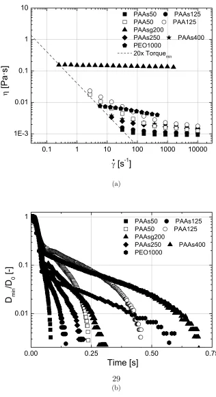
All these fluids were characterized rheologically under simple shear flow
92
by means of a rotational rheometer (Physica MCR301, Anton Paar) to
deter-93
mine the dependence of the shear viscosity on the shear rate (Figure 2a). In
94
this experiment the first normal stress difference (N1) can also be determined
95
from the measured normal force. However, measuringN1 in dilute and
semi-96
dilute polymer solutions is rather difficult and obtaining reproducibility in
97
the results is challenging. In these cases, it is more effective to perform the
98
characterization under uniaxial elongational flow as in a capillary-breakup
99
extensional rheometer (Haake CaBER1, Thermo Scientific), which measures
100
the time evolution of the diameter of a stretched fluid filament as it thins,
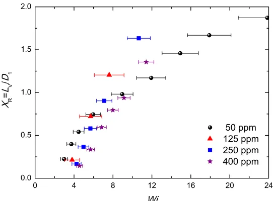
101
from which the longest relaxation time of the fluids can be determined (Figure
102
2b) [22]. Despite the significant differences between a steady shear flow (as
103
in a shear rheometer) and an unsteady extensional flow (as in the CaBER
104
device), there is a direct relationship between the elastic properties
mea-105
sured in both devices. Indeed, Zell et al. [23] have found that the normal
106
stress coefficient, measured in shear flow and defined as Ψ10 = N1
˙
γ2, shows
107
a quadratic dependence on the relaxation time determined in the CaBER.
108
Since the normal stress difference coefficient depends on a shear relaxation
109
time, the relation between the shear and extensional relaxation times may
4 5 6 7 8 9 10 11 12 13 14 15 16 17 18 19 20 21 22 23 24 25 26 27 28 29 30 31 32 33 34 35 36 37 38 39 40 41 42 43 44 45 46 47 48 49 50 51 52
seem obvious but there are different dependences that remain unexplained
111
as discussed by Zell et al. [23].
112
113
The viscoelastic fluids used in the experiments usually exhibit a shear
114
thinning behaviour, i.e. their apparent shear viscosity decreases with the
in-115
crease in the applied shear rate. Moreover, the higher the molecular weight
116
and the concentration of the polymer additive, the higher the shear viscosity,
117
the stronger the shear thinning behaviour and the longer the relaxation time
118
will be [24, 25]. These effects are clearly shown in Figure 2, where the
viscos-119
ity of the various fluids is plotted as a function of the shear rate in Figure 2a
120
and the time evolution of the normalized diameters measured in the CaBER
121
device are shown in Figure 2b. A small percentage of glycerol was added to
122
one of the fluids, in order to increase slightly the viscosity of the solution
123
increasing in turn the relaxation time of the polymer solution. Typically,
124
Boger fluids are prepared by dissolving a flexible polymer with large
molec-125
ular weight in a high viscosity solvent, to minimize the shear thinning due
126
to the addition of the polymer. However, the use of high-viscosity fluids in
127
microfluidics is precluded by the large pressure drops their flows develop with
128
severe consequences to the structural integrity of the chips. The advent of
129
Boger fluids with low viscosity is a useful alternative for microfluidics when
130
it is important to distinguish between shear thinning and elastic effects. By
131
adding salt to aqueous solutions of polyacrylamide, Aitkadi et al. [26] found
132
that the salt has a stabilizing effect on the shear viscosity while maintaining
133
adequate levels of elasticity, thus resulting in a Boger fluid behaviour, a good
134
example being the PAAsg200 fluid shown in Figure 2.
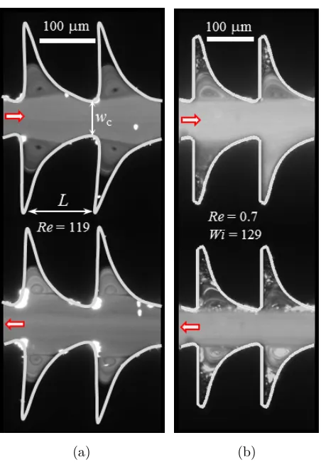
4 5 6 7 8 9 10 11 12 13 14 15 16 17 18 19 20 21 22 23 24 25 26 27 28 29 30 31 32 33 34 35 36 37 38 39 40 41 42 43 44 45 46 47 48 49 50 51 52
No storage or loss moduli (G and G) are presented because it was not
pos-136
sible to measure G accurately in small amplitude oscillatory shear (SAOS)
137
in this rotational rheometer due to instrument limitations and the low
elas-138
ticity of the fluids used. All the rheological experiments, as well as all the
139
microfluidic experiments, were performed at a constant temperature of 20 °C.
140
141
The geometries used were planar micro-channels made of
polydimethylsilox-142
ane (PDMS) fabricated from SU-8 photoresist moulds using standard
soft-143
lithography techniques, as described in [27, 28]. The micro-fabrication
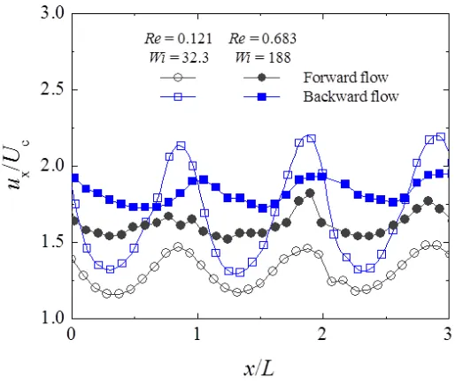
pro-144
cess consists of four fundamental steps: 1) drawing of the micro-geometries
145
using a CAD software; 2) manufacture of the mask using the CAD drawings
146
- this type of mask is obtained by sputtering a chrome layer onto a glass or
147
quartz substrate in which the CAD image is etched; 3) manufacture of the
148
SU-8 mould by photolithography using the mask; and 4) fabrication of the
149
PDMS micro-channels using the mould. High-resolution chrome masks were
150
employed to obtain high quality SU-8 moulds with nearly vertical side-walls
151
and well-defined corner features. The SU-8 photoresist was used to create
152
a positive-relief on the mould surface, producing a mould containing the
in-153
verse structure of the micro-channels. The microfluidic devices were then
154
fabricated by casting PDMS on the mould. The PDMS used (Sylgard 184,
155
Dow Corning) is commercially available as a prepolymer kit composed of a
156
PDMS oligomer and a crosslinking agent or curing agent, which are mixed
157
in certain proportions (typically 50:1, 20:1 and 10:1 PDMS:curing agent) to
158
produce the polymer used to fabricate the micro-devices. An overview of the
159
micro-channel fabrication procedure is shown schematically in Figure 3. In
4 5 6 7 8 9 10 11 12 13 14 15 16 17 18 19 20 21 22 23 24 25 26 27 28 29 30 31 32 33 34 35 36 37 38 39 40 41 42 43 44 45 46 47 48 49 50 51 52
the next section the different geometrical arrangements and their influence
161
on the fluid flow will be described in detail. Figure 4 shows scanning electron
162
microscopy (SEM) pictures of the micro-channels used and Table 2 lists the
163
corresponding dimensions.
164
Pressure measurements were performed using differential pressure
transduc-165
ers (Honeywell 26 PC sensors) operating up to a maximum differential
pres-166
sure of 210 kPa. Pressure transducers with different ranges and sensitivities
167
were used depending on the fluids and flow rates tested. The flow rate was
168
always imposed using a syringe pump, such as the neMESYS (Cetoni GmbH)
169
and PHD 2000 (Harvard Apparatus), equipped with different Hamilton
sy-170
ringes (from 25μl to 1ml, depending on the required flow rate) to ensure
171
pulsation-free dosing.
172
Flow visualizations were based on streak photography with the micro-channels
173
placed on the motorized stage of an inverted epi-fluorescence microscope
174
(DMI 5000M, Leica Microsystems GmbH) equipped with a sensitive
monochro-175
matic CCD camera (DFC350 FX, Leica Microsystems GmbH). The fluids
176
were seeded with fluorescent tracer particles (1 μm diameter Nile Red
par-177
ticles, Molecular Probes, Invitrogen, Ex/Em: 520/580 nm) and the
illu-178
mination was provided by a 100 W mercury lamp operating together with
179
adequate excitation and emission filters and a dichroic mirror.
180
For the velocity measurements, a micro-Particle Image Velocimetry (μPIV)
181
system from Dantec Dynamics was used. Images of the emitted radiation
182
from excited fluorescent tracer particles were captured using a 20×
(numer-183
ical aperture, NA=0.4) microscope objective and a camera (Flow Sense 4M,
184
Dantec Dynamics), with a resolution of 2048 × 2048 pixels and running on
4 5 6 7 8 9 10 11 12 13 14 15 16 17 18 19 20 21 22 23 24 25 26 27 28 29 30 31 32 33 34 35 36 37 38 39 40 41 42 43 44 45 46 47 48 49 50 51 52
double frame mode. The flow was illuminated by a double-pulsed 532 nm
186
Nd:YAG laser (Dual Power 65-15, Dantec Dynamics). The fluorescent
par-187
ticles used in μPIV were smaller than those used in streak photography and
188
had a diameter of 0.5 μm.
189
3. Results and Discussion
190
In this section, we review five different experimental investigations in
extensional-191
dominated flows of viscoelastic fluids which explore the onset of elastic
insta-192
bilities. The case studies focus on fundamental issues to understand the flow
193
dynamics itself, but also cover more applied research ranging from fluid
char-194
acterization in a microfluidic rheometer to the development of a microfluidic
195
diode, which can be used as a flow rectifier or in micro-pumps.
196
3.1. Microfluidic hyperbolic contraction and sudden expansion
197
The flow of Boger fluids in hyperbolic contraction micro-channels was
in-198
vestigated to assess the relation between the observed flow patterns and the
199
dimensionless relaxation time of the fluids. The underlying rationale for
us-200
ing hyperbolic-shaped channels is their ability to generate strong extensional
201
flows with enhanced strain-rate homogeneity near the centreline when
com-202
pared to other contraction flows [29, 30]. This geometry is thus sensitive
203
to effects of elongational viscosity and the use of Boger fluids allows a clear
204
separation between elastic and viscous effects [31].
205
In their investigation on the flow through hyperbolic contraction and sudden
206
expansion, Campo-Dea˜no et al. [32] used aqueous solutions of PAA at
differ-207
ent weight concentrations (50, 125, 250 and 400 ppm) to which 1% of NaCl
208
were added (Table 1). The shear viscosity of the fluids ranges from 1 to 4
4 5 6 7 8 9 10 11 12 13 14 15 16 17 18 19 20 21 22 23 24 25 26 27 28 29 30 31 32 33 34 35 36 37 38 39 40 41 42 43 44 45 46 47 48 49 50 51 52
mPa·s (Figure 2).
210
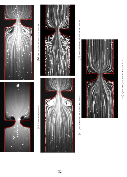
The geometry imaged in Figure 4a) includes a hyperbolic contraction
fol-211
lowed by a sudden expansion. The width of the inlet and outlet channels is
212
D1=400 μm, the minimum width of the contraction is D2=54 μm and the
213
length of the hyperbolic contraction region is Lc=128 μm, resulting in a
to-214
tal Hencky strain of εH= ln(D1/D2)=2. The depth of the micro-channel is
215
constant, h= 45 μm.
216
Visualizations of the flow patterns in the hyperbolic contraction/abrupt
ex-217
pansion micro-channel (Figure 5) showed a Newtonian-like behaviour at very
218
low flow rates (low W i) and complex non-Newtonian behaviour at high flow
219
rates (high W i) for all polymer concentrations. This non-Newtonian
be-220
haviour corresponds to the existence of regions of separated flow upstream of
221
the contraction. Thus, for negligible inertia and elasticity no flow separation
222
was observed. For the Boger fluid with 400 ppm of PAA and 1% NaCl the
223
critical flow rate at which the behaviour first changes from Newtonian-like to
224
non-Newtonian was determined as Qcr = 0.17 ml/hr, which corresponds to
225
Re = 0.7 andWi = 4; for the PAA solution at 250 ppm the critical value is
226
Qcr = 0.27 ml/hr (Re = 1.2,Wi = 4); for 125 ppm Qcr = 0.47 ml/hr (Re =
227
2.8, Wi = 3.6), and finally for the lowest concentration of 50 ppm the critical
228
flow rate corresponds to Qcr = 0.95 ml/hr (Re = 5.8, Wi = 2.8). Figure 5
229
shows flow patterns above this critical flow rate for each case. As expected,
230
there is a clear decrease in the critical flow rate when the polymer
concentra-231
tion is increased due to enhanced elasticity with the corresponding increase
232
of the relaxation time. However, the transition was found to correspond to
233
a critical value of Wi of about 4, which did not decrease significantly except
4 5 6 7 8 9 10 11 12 13 14 15 16 17 18 19 20 21 22 23 24 25 26 27 28 29 30 31 32 33 34 35 36 37 38 39 40 41 42 43 44 45 46 47 48 49 50 51 52
when flow inertia became relevant (Re>2). Above the critical flow rate,
sym-235
metric vortices develop upstream of the hyperbolic contraction in contrast
236
to the behaviour of Newtonian liquids that exhibit vortices downstream as a
237
consequence of inertial effects. Further increasing the Weissenberg number
238
leads to an increase of the upstream vortex due to the enhancement of
elas-239
tic effects which is characterized in terms of the dimensionless vortex length,
240
XR=Lv/D1, where Lv is the vortex length. This variation ofXR with W iis
241
shown in Figure 6 and it can be used as a simple methodology to estimate
242
the value of the relaxation time for solutions of very low polymer
concentra-243
tion by doing an extrapolation from the relaxation time obtained using the
244
extensional rheometer (CaBER) for the highest concentrations (400 and 250
245
ppm) to the lowest concentration (50 ppm) based on the assumption that
246
W icr is essentially independent of the polymer concentration. This
assump-247
tion is expected to hold as long as inertial effects are not important. In this
248
case, as the critical Weissenberg number is W icr ≈4, the relaxation time for
249
the 50 ppm solution can be estimated using Equation 2:
250
W icr =λ˙≈ λ(U2−U1)
Lc =λ Qcr hLc
1
D2 −
1
D1
(2)
obtaining λ ≈5 ms, which is similar to the value measured in the CaBER
251
(λ= 4±1 ms).
252
As already discussed, at high Wi an increase of the vortex size due to the
253
progressive enhancement of elastic effects is observed. Moreover, in the
ex-254
periments reported by McKinley et al. [33], and Sousa et al. [34] using a
255
different aqueous polymer solution (PEO), the vortex growth upstream of
256
the contraction presents either asymmetric and/or time-dependent behaviour
4 5 6 7 8 9 10 11 12 13 14 15 16 17 18 19 20 21 22 23 24 25 26 27 28 29 30 31 32 33 34 35 36 37 38 39 40 41 42 43 44 45 46 47 48 49 50 51 52
which increases in magnitude with W i, while in the present case the flows
258
are still steady and symmetric at the flow rates studied, as they are below
259
the critical point.
260
This vortex growth regime in viscoelastic fluid flows in contractions has been
261
also widely reported at the macro-scale. For instance, Alves et al. [35] used a
262
more viscous Boger fluid to characterize the flow patterns in a square-square
263
contraction, observing the formation of vortices upstream the contraction
264
plane at low De (or low W i) which increased with De until the flow
be-265
came chaotic-like at high flow rates. Note that these flows were also
char-266
acterized by small Reynolds numbers, Re<1. Rothstein and McKinley [36]
267
studied experimentally the flow of a Boger fluid in an axisymmetric
contrac-268
tion/expansion and they also reported an increase in the normalized pressure
269
drop at high De which is believed to be the result of an additional resistance
270
due to the extensional flow in the contraction (strain-hardening of the
ex-271
tensional viscosity). Later on, Sousa et al. [37] studied the flow of a Boger
272
fluid through square-square contractions with different contraction ratios,
273
and identified a number of distinct flow type regions with increasing values
274
of De: at lowDe a region in which lip and corner vortices coexist followed at
275
higherDe by two distinct regions of diverging flow which are associated with
276
vortex growth but exhibit different characteristics for low and high
contrac-277
tion ratios; and at large De the onset of unstable flow in which the vortex
278
size varies periodically in time.
279
3.2. Microfluidic diode
280
A microfluidic diode, or rectifier, is a micro-channel with anisotropic flow
281
resistance in both flow directions. The anisotropic behaviour can be due to
4 5 6 7 8 9 10 11 12 13 14 15 16 17 18 19 20 21 22 23 24 25 26 27 28 29 30 31 32 33 34 35 36 37 38 39 40 41 42 43 44 45 46 47 48 49 50 51 52
inertial or elastic up-aft symmetry breaking effects when Newtonian or
vis-283
coelastic fluids flow in these micro-devices, respectively. Microfluidic diodes
284
can be employed for instance in fixed geometry micro-pumps, which are
285
commonly used in micro total analysis systems (μTAS) for pumping fluids
286
[38, 39]. The first fluidic rectifier was patented by Tesla [40] for Newtonian
287
fluids based on inertial non-linear effects at high Reflows.
288
For viscoelastic fluids, Groisman and Quake [41] proposed a microfluidic
de-289
vice consisting of 43 triangular cavities connected in series, which exhibited
290
a maximum diodicity (Di) of about 2 (Di is defined as the ratio between
291
the backward, higher, and forward, lower, flow rates through the device for
292
a given pressure drop). Later, a significant increase in the diodicity was
293
achieved by Sousa et al. [42, 43], using microfluidic diodes made from 42
294
similar hyperbolic shaped cavities connected in series, using different aspect
295
ratios. The aspect ratio (AR) is defined as the ratio between the depth of the
296
channel and its smallest width (wc) at the neck of the contraction (cf. Figure
297
7a for the geometry of a single element) and microfluidic diodes with AR =
298
0.73, 1.26 and 1.71 were used in the experiments. The viscoelastic fluid used
299
was an aqueous solution of PEO at a concentration of 0.1 wt% (Table 1). The
300
polymer solution (PEO1000 in Figure 2) has a shear-thinning behaviour with
301
a zero-shear rate viscosity of η0= 7.5 mPa·s, an infinite shear rate viscosity
302
of η∞= 3 mPa·s and a relaxation time determined in the CaBER device, λ
303
= 73.9 ms (Figure 2b). The Reynolds number is defined as Re = ρUcwc/η0,
304
where Uc is the average velocity at the narrow passage with width wc, and
305
the Weissenberg number is defined as W i=λUc/(wc/2).
306
The flows are characterized by low Re and under these conditions the flow of
4 5 6 7 8 9 10 11 12 13 14 15 16 17 18 19 20 21 22 23 24 25 26 27 28 29 30 31 32 33 34 35 36 37 38 39 40 41 42 43 44 45 46 47 48 49 50 51 52
the Newtonian fluid is found to be similar in both flow directions as in the
308
limit of Re→0 due to creeping flow reversibility, hence the diodicity is one.
309
Recirculations appear in both flow directions and grow within the hyperbolic
310
elements as Re is increased, but the flow remains symmetric relative to the
311
centreline, as shown in Figure 7a, with no significant rectification effects.
312
For the viscoelastic fluid flow we observed an entirely different dynamic flow
313
behaviour, with elasticity-induced recirculations appearing inside the
hyper-314
bolic corners, except at low flow rates (lowWi) where the flow is
Newtonian-315
like. As the elasticity is increased, elastic instabilities appear first in the
316
forward direction as shown in Figure 7b and only at higher W i do they
ap-317
pear in reversed flow. With the onset of the elastic instabilities, the vortices
318
appear and disappear along time in some elements of the diode (unsteady
319
flow). The critical Weissenberg number (W icr) for the onset of these elastic
320
instabilities in forward flow increases with the depth of the channel (h): for
321
AR= 0.73,W icr≈ 20; for AR = 1.26,W icr≈ 25; and forAR = 1.71,W icr≈
322
45.
323
Profiles of the normalized streamwise velocity measured with μ-PIV along
324
the centreline of several consecutive elements show a large difference in the
325
amplitude of the velocity oscillations in both flow directions, as can be seen in
326
Figure 8. This dissimilar behaviour in the two directions is in contrast to the
327
results for Newtonian fluids where the amplitudes of the oscillations of the
328
velocity profiles in backward and forward flow were the same, as documented
329
by Sousa et al. [42] and not shown here for conciseness. In the backward
di-330
rection, for which the viscoelastic flow remains steady up to higher flow rates,
331
the velocity gradient at the centreline is higher than for the forward direction
4 5 6 7 8 9 10 11 12 13 14 15 16 17 18 19 20 21 22 23 24 25 26 27 28 29 30 31 32 33 34 35 36 37 38 39 40 41 42 43 44 45 46 47 48 49 50 51 52
(unsteady flow). Note that in the latter case the velocity field was averaged
333
over a long period of time, in which the flow behaviour was varying in time
334
due to the elastic instability and consequently, the velocity oscillations were
335
smoothed. In those unsteady flow experiments, time-averaged measurements
336
were made over a time scale significantly larger than the fluid relaxation time
337
to establish the overall time-averaged flow field.
338
For viscoelastic fluid flow, the pressure drop measured along the
micro-339
channel also depends on the flow direction, leading to enhanced diodicity.
340
As shown in Figure 9a, the pressure drop is higher in the forward direction,
341
where the flow is more sensitive to elastic instabilities leading to unsteady
342
flow at lower Wi than in the backward flow direction, so that the diodicity
343
increases significantly above this first flow transition. At higher flow rates
344
(or Wi), when the flow also becomes unsteady in the backward direction,
345
the corresponding pressure drop ceases to differ so significantly from that in
346
the forward direction leading to a reduction of diodicity at high W i. The
347
stronger and more homogeneous extensional flow in the forward direction is
348
responsible for the earlier onset of elastic instabilities and of enhanced
diod-349
icity (Di), especially for higher aspect ratios as shown in Figure 9b. Using
350
the hyperbolic-shaped micro-devices a maximum diodicity of about 6.4 was
351
achieved when the effect of the bounding walls decreased, thus minimizing
352
shear effects and enhancing the extensional flow component [42].
353
3.3. Flow-focusing device
354
The geometry of a flow-focusing device is similar to a cross-slot device, but
355
the flow comprises three inlets and one outlet channel (all of width D, cf.
356
Figure 4c), thus imposing an extensional flow to the central stream of the
4 5 6 7 8 9 10 11 12 13 14 15 16 17 18 19 20 21 22 23 24 25 26 27 28 29 30 31 32 33 34 35 36 37 38 39 40 41 42 43 44 45 46 47 48 49 50 51 52
device, as shown in the Newtonian fluid flow patterns of Figure 10. This
358
geometry has been used at the micro-scale for a number of applications, such
359
as rheometry [44], fluid mixing [45], or droplet formation [46].
360
We investigated experimentally the flow of a Newtonian fluid, de-ionized
wa-361
ter [47, 48], and of a viscoelastic fluid [47], which was an aqueous solution of
362
125ppm (w/w) of PAA with 1% of NaCl (Table 1) resulting in a Boger-like
363
fluid with a nearly constant viscosity ofη= 1.31 mPa·s and a relaxation time
364
ofλ= 12.4 ms, measured in the CaBER device (Figure 2). For the Newtonian
365
fluid flow, Figure 10 compares the experimental flow patterns with numerical
366
predictions obtained at the same flow conditions showing a very close match.
367
The Newtonian fluid flow remained symmetric relative to the horizontal
cen-368
treline (cf. Figure 10) for a wide range of flow conditions (Re 113). The
369
Reynolds number, based on the exit channel, is defined as Re = ρU3D3/η,
370
where U3 and D3 are the corresponding average velocity and channel width.
371
Furthermore, the flow rate ratio (F R =Q2/Q1) or the corresponding velocity
372
ratio (V R=V2/V1), defined as the ratio of the inlet average velocities in the
373
lateral streams to the average velocity in the central inlet stream, controls
374
the total Hencky strain experienced by the fluid in the converging region [47]
375
(shown by separation streamlines in Figure 10).
376
For the viscoelastic fluid, a symmetric flow was also observed but only at
377
sufficiently low Wi as shown in Figure 11a. As Wi is increased (defined as
378
Wi =λU3/D3), two types of instabilities were observed [48]: a first transition
379
in which the steady symmetric flow becomes asymmetric but remains steady
380
(Figure 11b) and a second instability at higherW iin which the steady
asym-381
metric flow becomes unsteady (Figure 11c).
4 5 6 7 8 9 10 11 12 13 14 15 16 17 18 19 20 21 22 23 24 25 26 27 28 29 30 31 32 33 34 35 36 37 38 39 40 41 42 43 44 45 46 47 48 49 50 51 52
The first transition is driven by elastic normal stresses that act along the
383
streamlines and is entirely absent from the corresponding Newtonian fluid
384
flow. Compared to the cross-slot flow discussed by Poole et al. [49], the main
385
differences lie in the fact that there is no stagnation point at the centre of the
386
geometry and that the onset of elastic driven instabilities depends not only
387
on Wi, but also on the velocity ratio as shown in Figure 12. For example,
388
we observed that for very low VRthe flow evolves directly from steady
sym-389
metric to unsteady flow without ever going through the intermediate regime
390
of steady asymmetric flow. This behaviour was also captured in the numeric
391
computations [19] and was attributed to the normal stresses not being
suf-392
ficiently high to trigger that intermediate transition. The transition from
393
steady symmetric to steady asymmetric flows acts therefore as a stress relief
394
mechanism.
395
396
3.4. Confined cylinder
397
The flow past a cylinder is a classic problem in fluid dynamics. The shallow
398
depths typical of microfluidics bring a renewed interest into this topic, in
399
particular on the effects of the aspect ratio. The flow of a Newtonian and
400
a viscoelastic Boger fluid past a confined cylinder of diameter D placed in
401
the centre of a micro-channel (width H = 212 μm, cf. Figure 4d) was
in-402
vestigated to assess the effects of the blockage ratio (BR, ratio between the
403
cylinder diameter and the width of the microfluidic device) and aspect
ra-404
tio (AR, ratio between the depth of the microfluidic device and the cylinder
405
diameter). To characterize the Boger fluid flow we use the Weissenberg
num-406
ber, W i = λU/(D/2) and when necessary the Reynolds number is defined
4 5 6 7 8 9 10 11 12 13 14 15 16 17 18 19 20 21 22 23 24 25 26 27 28 29 30 31 32 33 34 35 36 37 38 39 40 41 42 43 44 45 46 47 48 49 50 51 52
asRe=ρUD/2η. The micro-geometries were designed with different widths
408
and depths to obtain AR= 2.0, 1.0 and 0.55 and BR = 25%, 50% and 75%.
409
De-ionized water was used as Newtonian fluid and the Boger fluid was an
410
85 wt% aqueous solution of glycerol and PAA at a weight concentration of
411
200 ppm with 1% NaCl (Table 1). The Boger fluid showed a nearly constant
412
shear viscosity of 0.152 Pa·s over a wide range of shear rates. The
character-413
istic relaxation time of the Boger fluid measured in the CaBER device was
414
λ = 86.7 ms at 293.2 K (Figure 2b).
415
For the Newtonian fluid flow at creeping flow conditions, there is no flow
416
separation and the flow patterns are symmetric both upstream and
down-417
stream of the cylinder, due to creeping flow reversibility of Newtonian flows.
418
At non-negligible Reynolds numbers, the measurements confirm the onset of
419
flow separation downstream of the cylinder above a critical value of Re, in
420
agreement with Ribeiro et al. [50]. This critical Re depends onAR and BR
421
and increases with BR with a more pronounced effect at higher BR.
422
Over the wide range ofWi investigated the following flow regimes were
iden-423
tified: Newtonian-like flow; flow with steady divergent streamlines; periodic
424
flow; chaotic-like flow. This sequence of flow transitions takes place as Wi
425
is increased and the critical conditions for the transitions were found to be
426
dependent onAR and BR. For lowWi, regardless of ARand BR, the flow is
427
always symmetric upstream and downstream of the cylinder. Increasing Wi,
428
diverging streamlines progressively appear upstream of the cylinder. Both
429
the critical conditions for the onset of the diverging streamlines and the
in-430
tensity of this effect depend on the values ofARandBR: Figure 13 illustrates
431
that for BR=50% and Wi≈ 30 the intensity of the diverging streamlines
4 5 6 7 8 9 10 11 12 13 14 15 16 17 18 19 20 21 22 23 24 25 26 27 28 29 30 31 32 33 34 35 36 37 38 39 40 41 42 43 44 45 46 47 48 49 50 51 52
creases as AR decreases. Moreover, we also found that for the same Wi, the
433
intensity of the divergent streamlines increases asBRincreases. Therefore, in
434
both cases the divergent streamlines become stronger with wall confinement.
435
AsWiincreases further, the divergent streamlines become progressively more
436
pronounced until an elastic instability arises upstream of the cylinder, near
437
the forward stagnation point, leading to time-dependent flow. For the range
438
of flow conditions tested, elastic instabilities were observed only for BR=
439
75%. Figure 14 shows the profiles of the streamwise dimensionless velocity
440
along the centreline for the Boger fluid flow in order to illustrate the effects
441
of: elasticity at constant AR and BR (Figure 14a) and of the aspect ratio
442
for constant Wi and BR (Figure 14b).
443
The streamwise velocity far upstream of the cylinder is similar to that of
444
the Newtonian fluid flow, since the shear viscosity is constant and the shape
445
of the fully-developed velocity profile is exclusively determined by the shear
446
stress. Upstream of the cylinder the Boger fluid flow is independent of the
447
elasticity of the fluid (cf. Figure 14a), but it naturally depends on the aspect
448
ratio of the inlet channel (cf. Figure 14b) with the maximum velocity of the
449
fully-developed profile occurring for AR = 2 (square channel). Downstream
450
of the cylinder, the length required for flow redevelopment increases
progres-451
sively with Wi (cf. Figure 14a),regardless of AR and BR. Figure 14b shows
452
that as geometric confinement increases the spatial influence of the cylinder
453
grows: the flow deceleration upstream of the cylinder starts slightly earlier
454
and the downstream flow redevelopment length increases.
4 5 6 7 8 9 10 11 12 13 14 15 16 17 18 19 20 21 22 23 24 25 26 27 28 29 30 31 32 33 34 35 36 37 38 39 40 41 42 43 44 45 46 47 48 49 50 51 52
3.5. Microfluidic analogues of a porous medium
456
Over the last decades, the flow of non-Newtonian fluids through porous
me-457
dia has gained significant importance in applications related to the petroleum
458
industry, as in enhanced oil recovery, among others. The combination of the
459
non-linear properties of those fluids with the meandering paths within the
460
media, thus combining shear and extensional flow features, results in a
com-461
plex fluid mechanics problem. Moreover, the porous media are typically
462
opaque thus preventing the use of optical techniques. In order to obtain a
463
better insight about the dynamics of viscoelastic fluid flows through porous
464
media we designed simple micro-channel analogues consisting of a sequence
465
of contractions/expansions arranged in symmetric and asymmetric
configu-466
rations as shown in Figure 4e [51]. Dilute aqueous solutions of PAA at 50
467
and 125ppm (Table 1 and Figure 2) were used as model viscoelastic fluids in
468
the porous media analogues, as well as in the real porous media consisting
469
of unconsolidated packed beds (beach sand).
470
Measurements with de-ionized water flowing through symmetric and
asym-471
metric micro-channels showed a linear variation of the streamwise pressure
472
gradient with the flow rate under laminar flow conditions. Using Darcy’s law
473
it was possible to relate the modified permeabilities of the micro-channels
474
with the permeability of the porous medium while obtaining the porosity of
475
the porous medium and the Sauter’s mean diameter (x32) of the particles as
476
described in [51]. It was found that the bed of beach sand with an average
477
particle size of x32 ≈ 400 μm and a porosity = 0.36 is characterized by
478
a modified permeability of kP M =2.8×10⁻¹⁰ m2, which is similar to the
per-479
meability of the analogue micro-channel. The results plotted in Figure 15a
4 5 6 7 8 9 10 11 12 13 14 15 16 17 18 19 20 21 22 23 24 25 26 27 28 29 30 31 32 33 34 35 36 37 38 39 40 41 42 43 44 45 46 47 48 49 50 51 52
show that both micro-channel configurations mimic well the pressure
drop-481
flow rate variation for Newtonian fluids when the equivalent particle size is
482
selected properly, corroborating in this way and in terms of these flow
prop-483
erties at least, that both simplified microfluidic systems are reasonably good
484
analogues of a real porous medium when a Newtonian fluid is used.
485
For viscoelastic fluids the situation is somehow different (Figure 15b). Here,
486
the Weissenberg number is defined asW i=λ Ui
dpMC, whereλis the relaxation
487
time of the fluid, Ui is the velocity in the contraction sections and dpM C is
488
the equivalent particle size of the analogous porous medium. At low W i, the
489
pressure drop measured experimentally across the bed varies linearly with
490
flow rate, but above a critical Weissenberg number (W icr), a larger slope in
491
the pressure gradient curve is observed due to the onset of elastic
instabili-492
ties in both the asymmetric micro-channel and real porous medium (critical
493
conditions depend on the geometry, see Figure 16). According to the
Pakdel-494
McKinley criterion [14, 15, 17], since the flow in the asymmetric configuration
495
is characterized by more marked streamline curvatures, the onset of elastic
496
instabilities is expected to occur at lower W i as found in the experiments.
497
The symmetric configuration was found to reproduce well the flow of
vis-498
coelastic fluids at low Wi, whereas the asymmetric configuration provides
499
better results at high Wi (Figure 15b). In this way, both micro-geometries
500
seem to be complementary and could be interesting tools to obtain a better
501
insight about the flow of viscoelastic fluids through a porous medium.
502
Finally, on the pursuit of analysing the elastic instabilities without the
influ-503
ence of shear thinning effects, we have also studied the flow of low-viscosity
504
Boger fluids (aqueous solutions of 50 and 125 ppm of PAA with 1% of NaCl,
4 5 6 7 8 9 10 11 12 13 14 15 16 17 18 19 20 21 22 23 24 25 26 27 28 29 30 31 32 33 34 35 36 37 38 39 40 41 42 43 44 45 46 47 48 49 50 51 52
see Table 1 and Figure 2 cf. [32]), through the same porous medium. Above
506
a critical flow rate, there is a large increase in the slope of the pressure
gra-507
dient curve (cf. Figure 17) due to the onset of elastic effects as discussed
508
previously. Then further increasing the flow rate, a more dramatic rise in
509
the slope of the pressure gradient vs. flow rate curve arises, i.e. showing an
510
unexpected very large third slope (Figure 17). This third slope could not
511
be reproduced in any of the microfluidic analogues of a porous medium and
512
was found to be related to the blocking of the porous medium due to the
513
apparent formation of a gel under these very extreme flow conditions [52].
514
4. Conclusions
515
The small size of microfluidic devices implies that often their flows are
char-516
acterized by low Reynolds numbers especially when the fluids contain
addi-517
tives that increase their viscosity. In addition, such additives usually impart
518
non-Newtonian behaviour and in particular elasticity to the fluid, leading
519
to high Weissenberg number flows in micro-channels. These are ultimately
520
responsible for the appearance of elastic instabilities at low or even
negligi-521
ble Reynolds numbers. This work summarizes five experimental
investiga-522
tions on pressure driven flows in micro-geometries that generate flows with
523
a non-negligible component of extensional deformation and where the onset
524
of various elastic instabilities are observed.
525
In all the symmetric geometries used the flows are Newtonian-like, steady
526
and symmetric at low Weissenberg numbers. However, upon increasing the
527
Weissenberg number elastic instabilities set in and the flow either becomes
528
steady asymmetric or unsteady. When a transition to steady asymmetric
4 5 6 7 8 9 10 11 12 13 14 15 16 17 18 19 20 21 22 23 24 25 26 27 28 29 30 31 32 33 34 35 36 37 38 39 40 41 42 43 44 45 46 47 48 49 50 51 52
flow takes place there is invariably a second elastic transition to unsteady
530
flow at a higher Weissenberg number. The path of transitions also depends
531
on other relevant dimensionless numbers specific to each geometric flow: for
532
flow-focusing it is possible to evolve directly from steady symmetric to
un-533
steady flow, without ever going through the steady asymmetric flow, for some
534
ranges of the velocity ratio and Reynolds number. Presumably, the different
535
transitions are associated with different mechanisms involving elastic normal
536
stresses. In some cases extremely high normal stresses lead to a specific flow
537
feature which is not observed under weaker flow conditions. In other cases
538
the curved streamlines are unable to sustain the normal stresses acting along
539
those streamlines as described by the Pakdel-McKinley criterion [14, 15, 17],
540
and the flow becomes unstable.
541
These elastic instabilities have both advantages and drawbacks in practical
542
terms. When the objective is micro-mixing or high rates of heat and mass
543
transfer, these low Reynolds number chaotic-like flows of elastic fluids provide
544
a useful solution which is not available if the fluids are Newtonian (a similar
545
situation here would require higher Reynolds numbers for chaotic advection
546
to emerge). However, if the objective is to minimize or delay the existence of
547
unstable flows, as when operating with micro-rheometers, then ideally there
548
should be no and these transitions impose operational limits.
549
As shown in the examples described, new phenomena arise at the micro-scale
550
when fluids are non-Newtonian and these flows have interesting features
espe-551
cially in combination with other unusual conditions not described here, such
552
as in the presence of electrokinetic effects or of gradients in surface tension
553
made possible by new developments and advances in micro-manufacturing
4 5 6 7 8 9 10 11 12 13 14 15 16 17 18 19 20 21 22 23 24 25 26 27 28 29 30 31 32 33 34 35 36 37 38 39 40 41 42 43 44 45 46 47 48 49 50 51 52
and surface coating methods. The popularity of micro-flow systems requires
555
the miniaturization of flow forcing methods and the use of electric and
mag-556
netic forcing mechanisms will certainly become more common as an
alter-557
native to pressure driven flow. The combination of these methods with
flu-558
ids made from complex additives, will certainly provide an opportunity to
559
explore new challenging phenomena. Already good examples are the
com-560
binations of microfluidics and optics (optofluidics) and of microfluidics and
561
acoustics (acousto-fluidics), for instance for particle mixing or separation in
562
micro-channels.
563
Acknowledgements
564
The authors acknowledge the funding from FCT, COMPETE and FEDER
565
through various projects and scholarships throughout the years:
PTDC/EQU-566
FTT/70727/2006, PTDC/EME-MFE/114322/2009, PTDC/EME-MFE/99109/2008
567
and PTDC/EQU-FTT/118716/2010, SFRH/BPD/69663/2010, SFRH/BPD/69664/2010,
568
SFRH/BPD/75258/2010, SFRH/BD/44737/2008, IF/00148/2013 and IF/00190/2013.
4 5 6 7 8 9 10 11 12 13 14 15 16 17 18 19 20 21 22 23 24 25 26 27 28 29 30 31 32 33 34 35 36 37 38 39 40 41 42 43 44 45 46 47 48 49 50 51 52
Table 1: Formulations of the viscoelastic fluids used.
Acronym
a Polymer Solvent
PAA PEO Water Glycerol NaCl λ
[ppm] [ppm] [%] [%] [%] [ms]
PAAs50 50 0 100 0 1 4±1
PAA50 50 0 100 0 0 54±1
PAAs125 125 0 100 0 1 10±2
PAA125 125 0 100 0 0 129±1
PAAsg200 200 0 85 15 1 87±1
PAAs250 250 0 100 0 1 18±2
PAAs400 400 0 100 0 1 29±2
PEO1000 0 1000 100 0 0 74±1
aPAA: Polyacrylamide; PAAs: PAA with NaCl in water; PAAsg: PAA in water with
4 5 6 7 8 9 10 11 12 13 14 15 16 17 18 19 20 21 22 23 24 25 26 27 28 29 30 31 32 33 34 35 36 37 38 39 40 41 42 43 44 45 46 47 48 49 50 51 52
Table 2: Dimensions of the micro-channels used in the works here reviewed (see Figure
4).
Hyperbolic contraction h[μm] D1[μm] D2[μm] Lc[μm]
(Fig.4a) 45 400 54 128
Microfluidic diode
AR[-] h[μm] D[μm] wc[μm] L[μm]
0.73 46 326 63 128
(Fig.4b) 1.26 88 326 70 128
1.71 120 326 70 128
Flow focusing h[μm] D[μm]
Fig.4c 100 100
Confined cylinder
AR[-] BR[%] h[μm] D[μm] H[μm]
0.37 75 58 158 212
0.55 55 58 105 212
1.1 25 58 55 212
0.66 75 105 158 212
(Fig.4d) 1.0 50 105 105 212
1.9 25 105 55 212
1.3 75 213 158 212
2.0 50 213 105 212
3.9 25 213 55 212
Analogues of a porous medium
W1[μm] W2[μm] Wc[μm] L1[μm] L2[μm] h[μm]
Symmetric arrangement
108 40 40 106 31 103
(Fig.4e) Asymmetric arrangement
[image:27.612.116.517.139.554.2]4 5 6 7 8 9 10 11 12 13 14 15 16 17 18 19 20 21 22 23 24 25 26 27 28 29 30 31 32 33 34 35 36 37 38 39 40 41 42 43 44 45 46 47 48 49 50 51 52
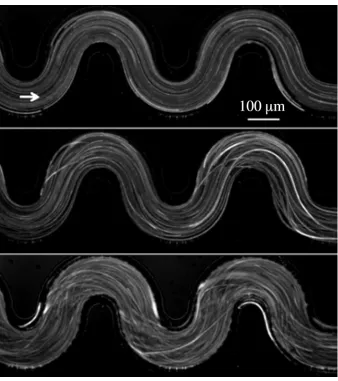
Figure 1: Illustration of the onset of an elastic instability frominstantaneous
flow patterns of a PEO solution in a 50:50 water/glycerol mixture flowing
through a serpentine channel (Mcrit≈0.68). From top to bottom: stable flow
(W i = 0.22); slightly unstable flow, close to the onset of elastic instability
(W i = 0.24); and unstable flow (W i = 0.25). Reproduced with permission
4 5 6 7 8 9 10 11 12 13 14 15 16 17 18 19 20 21 22 23 24 25 26 27 28 29 30 31 32 33 34 35 36 37 38 39 40 41 42 43 44 45 46 47 48 49 50 51 52
[image:29.612.135.451.96.675.2]4 5 6 7 8 9 10 11 12 13 14 15 16 17 18 19 20 21 22 23 24 25 26 27 28 29 30 31 32 33 34 35 36 37 38 39 40 41 42 43 44 45 46 47 48 49 50 51 52
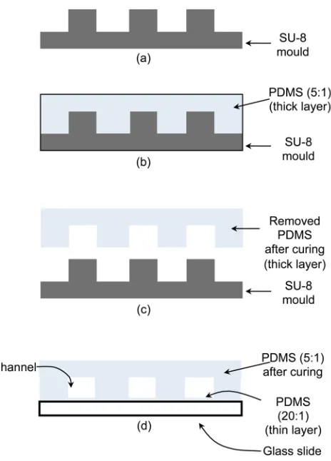
Figure 3: PDMS device fabrication procedure. (a) Cross-section of the SU-8
mould with a positive relief. (b) The mixture of oligomer and curing agent
is poured onto the SU-8 mould (thick layer) and placed in the oven to cure
for 20 minutes. (c) After curing, the PDMS thick layer is removed from the
SU-8 mould and access ports are created. (d) The PDMS layer containing
the channel structure is bonded to the glass slide covered with a thin layer
4 5 6 7 8 9 10 11 12 13 14 15 16 17 18 19 20 21 22 23 24 25 26 27 28 29 30 31 32 33 34 35 36 37 38 39 40 41 42 43 44 45 46 47 48 49 50 51 52
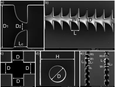
Figure 4: Scanning Electron Microscopy images of the five planar
micro-channels fabricated from high quality SU-8 photoresist moulds obtained by
means of a high-resolution chrome mask using standard soft lithography:
(a) hyperbolic contraction and sudden expansion; (b) microfluidic diode; (c)
cross-slot device (to be used as a flow focusing micro-device); (d) confined
cylinder; and (e) simplified microfluidic analogues of a porous medium. See
4 5 6 7 8 9 10 11 12 13 14 15 16 17 18 19 20 21 22 23 24 25 26 27 28 29 30 31 32 33 34 35 36 37 38 39 40 41 42 43 44 45 46 47 48 49 50 51 52
Figure 6: Effect of Weissenberg number on the dimensionless vortex length
in the steady symmetric regime for the 50, 125, 250 and 400 ppm PAA
aqueous solutions with 1% NaCl flowing through a hyperbolic-shaped
4 5 6 7 8 9 10 11 12 13 14 15 16 17 18 19 20 21 22 23 24 25 26 27 28 29 30 31 32 33 34 35 36 37 38 39 40 41 42 43 44 45 46 47 48 49 50 51 52
[image:34.612.193.419.71.400.2](a) (b)
Figure 7: (a) Newtonian fluid flow patterns in a hyperbolic diode with AR = 0.73.
Adapted from Sousa et al. [43]. (b) Viscoelastic fluid flow patterns in a microfluidic diode
4 5 6 7 8 9 10 11 12 13 14 15 16 17 18 19 20 21 22 23 24 25 26 27 28 29 30 31 32 33 34 35 36 37 38 39 40 41 42 43 44 45 46 47 48 49 50 51 52
Figure 8: Dimensionless axial velocity profiles along the centreline of the
microfluidic diode, AR = 0.73, for viscoelastic fluid flow under two different
flow rates. The streamwise velocity component (ux) is normalised with the
4 5 6 7 8 9 10 11 12 13 14 15 16 17 18 19 20 21 22 23 24 25 26 27 28 29 30 31 32 33 34 35 36 37 38 39 40 41 42 43 44 45 46 47 48 49 50 51 52
Figure 10: Experimental (micrograph) and numerical (red solid lines) flow
patterns obtained for Newtonian fluid flow in a flow-focusing micro-device,
Q1 = Q2 = 0.3 ml h−1, V R = 1 and Re = 2.8. The separation streamlines
are highlighted by white dashed lines and arrows indicate the flow direction.
4 5 6 7 8 9 10 11 12 13 14 15 16 17 18 19 20 21 22 23 24 25 26 27 28 29 30 31 32 33 34 35 36 37 38 39 40 41 42 43 44 45 46 47 48 49 50 51 52
1 10 100 1000
VR
0.00.5 1.0 1.5 2.0 2.5 3.0 3.5 4.0
Wi
0.0 0.4 0.8 1.2 1.6 2.0 2.4
Re
Unstable Flow
Flow Asymmetric
[image:39.612.136.475.76.306.2]Symmetric Flow
Figure 12: Flow classification map in theWi-VRdomain for the flow-focusing
micro-device. The circles indicate symmetric flow, the crosses steady
4 5 6 7 8 9 10 11 12 13 14 15 16 17 18 19 20 21 22 23 24 25 26 27 28 29 30 31 32 33 34 35 36 37 38 39 40 41 42 43 44 45 46 47 48 49 50 51 52
Figure 13: Flow patterns obtained for the Boger fluid flow around a cylinder
for BR = 50% as a function of AR under similar flow conditions: a) AR =
2.0, Wi = 30.5, Re= 7.8×10⁻³; b)AR= 1.0, Wi = 30.9, Re= 7.9×10⁻³; c)
4 5 6 7 8 9 10 11 12 13 14 15 16 17 18 19 20 21 22 23 24 25 26 27 28 29 30 31 32 33 34 35 36 37 38 39 40 41 42 43 44 45 46 47 48 49 50 51 52
(a
)
(b)
Figure
14:
Str
ea
m
wise
dimensio
nless
v
elo
cit
y
p
ro
files
a
lo
n
g
the
cen
tr
eline
o
f
the
flo
w
a
ro
und
a
co
nfined
cylinder
a
s
a
functio
n
of
el
ast
ici
ty
fo
r
AR
=1a
n
d
BR
=
50%
(a)
an
d
as
a
fu
n
ct
ion
of
AR
fo
r
Wi
=5a
n
d
BR
=
50%
.
(b
[image:41.612.117.333.87.634.2]4 5 6 7 8 9 10 11 12 13 14 15 16 17 18 19 20 21 22 23 24 25 26 27 28 29 30 31 32 33 34 35 36 37 38 39 40 41 42 43 44 45 46 47 48 49 50 51 52
(a)
[image:42.612.187.409.91.498.2](b)
Figure 15: Average pressure drop gradient as a function of the interstitial
ve-locity for the flow of (a) de-ionized water through the microfluidic analogues
of a porous medium (MCAsym, MCSym) and the porous sand bed (PM); (b) an
aqueous solution of PAA at 125ppm through the microfluidic analogues of a
4 5 6 7 8 9 10 11 12 13 14 15 16 17 18 19 20 21 22 23 24 25 26 27 28 29 30 31 32 33 34 35 36 37 38 39 40 41 42 43 44 45 46 47 48 49 50 51 52
Figure 16: Wi−Re flow pattern map for the symmetric micro-channel.
4 5 6 7 8 9 10 11 12 13 14 15 16 17 18 19 20 21 22 23 24 25 26 27 28 29 30 31 32 33 34 35 36 37 38 39 40 41 42 43 44 45 46 47 48 49 50 51 52
Figure 17: Variation of the pressure gradient with the interstitial velocity for
the flow of low viscosity Boger fluids through a porous medium made of sand
of 400 μm particles (Sauter mean diameter). Adapted from Campo-Dea˜no