Asymptotic and numerical analysis of a
simple model for blade coating
J. Quintans Carou, S. K. Wilson
∗, N. J. Mottram and B. R. Duffy
Department of Mathematics, University of Strathclyde,
Livingstone Tower, 26 Richmond Street, Glasgow,
G1 1XH, United Kingdom
3rd July 2007, revised 28th February 2008
Abstract
Motivated by the industrial process of blade coating, the two-dimensional flow of a thin
film of Newtonian fluid on a horizontal substrate moving parallel to itself with constant
speed under a fixed blade of finite length in which the flows upstream and downstream
of the blade are coupled via the flow under the blade is analysed. A combination of
asymptotic and numerical methods is used to investigate the number and nature of the
steady solutions that exist. Specifically, it is found that in the presence of gravity there
is always at least one, and (depending on the parameter values) possibly as many as
three, steady solutions, and that when multiple solutions occur they are identical under
and downstream of the blade, but differ upstream of it. The stability of these solutions
is investigated, and their asymptotic behaviour in the limits of large and small flux
and weak and strong gravity effects, respectively, determined.
∗Author for correspondence. Email: [email protected], Telephone: + 44 (0) 141 548 3820, Fax:
1
Introduction
During the industrial process of blade coating, a thin fluid film is applied to a moving
sub-strate by the action of a fixed blade (or vice versa). Blade coating is important because of
the wide range of products in whose manufacture it is used, including newspapers and
cata-logues, photographic films, magnetic storage media and fibres. The economic importance of
this process has motivated extensive research in order to understand better the underlying
physical mechanisms involved, and hence to improve its efficiency. In particular, various
mathematical models for blade coating have been developed in order to predict the form
and thickness of the final coated film. Ruschak [1] reviews some of the early mathematical
work on various fluid coating processes, and a more recent account of the large and
grow-ing literature on coatgrow-ing can be found in the encyclopaedic volume edited by Kistler and
Schweizer [2]. Regular scientific conferences on coating in Europe (the European Coating
Symposium: see, for example, [3]) and the USA (the International Coating Science and
Technology Symposium, [4]) attest to the ongoing interest and research activity in this area.
In the present paper we analyse a simple model of the blade-coating process consisting of
the two-dimensional flow of a thin film of Newtonian fluid on a horizontal substrate moving
parallel to itself with constant speed under a fixed blade of finite length in which the flows
upstream and downstream of the blade are coupled via the flow under the blade.
The starting point for the present analysis is the work of Moriarty and Terrill [5] who
investigated the same problem in the special case of a horizontal blade in the absence of
gravity, as an idealised model for the motion of a hard contact lens on the tear film in the
human eye. In particular, for their problem Moriarty and Terrill [5] predicted the existence of
none, one or two steady solutions, and in an associated paper McLeod [6] proved analytically
the existence and multiplicity of these solutions.
In the present paper we build on the work of Moriarty and Terrill [5] by using a
com-bination of asymptotic and numerical methods to show that accounting for the presence
of gravity has a significant effect on the number and nature of the steady solutions that
exist. Specifically, we find that in this case there is always at least one, and (depending on
solutions occur they are identical under and downstream of the blade, but differ upstream
of it. We discuss the stability of these solutions, and determine their asymptotic behaviour
in the limits of large and small flux and weak and strong gravity effects, respectively.
2
The mathematical model
2.1
Formulation
We consider steady, two-dimensional flow of a thin film of Newtonian fluid of constant density
ρ, viscosity µ and surface-tension coefficient γ on a horizontal substrate which is taken to
lie in the plane z = 0 and is moving parallel to itself with constant speed U (> 0) in
the positive x direction, where xyz are Cartesian coordinates. The fluid has a free surface
z =h(x), except where it flows underneath a fixed blade of finite length L and prescribed
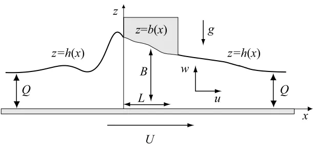
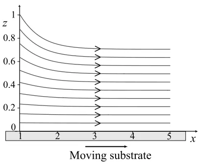
shape z = b(x) in 0 ≤ x ≤ L, as shown in Figure 1. The velocity v and pressure p are
written asv=v(x, z) = (u(x, z),0, w(x, z)) andp=p(x, z), and gravity acts in the negative
z direction. We use the following non-dimensionalisation:
x=Lx∗
, z =Bz∗
, b =Bb∗
, b0 =Bb
∗
0, bL=Bb∗1, h=Bh
∗
,
u=U u∗
, w= BU
L w
∗
, p−pa = µU L
B2 p
∗
, Q=U BQ∗
, (1)
whereB is a typical film thickness, b0 =b(0) and bL =b(L) denote the heights of the blade
at x = 0 and x = L, respectively, pa is the constant atmospheric pressure, and Q is the
constant volume flux of fluid (per unit width) in thex direction, given by
Q= Z b
0 udz for 0≤x≤L,
Z h
0 udz for x≤0 and x≥L.
(2)
Henceforth we drop the superscript stars from the non-dimensional variables.
We employ a thin-film approximation (see, for example, Ockendon and Ockendon [7,
Chapter 4]) based on the assumption that the aspect ratioof the film, defined by =B/L,
is small, that is,1. This assumption is well justified in many practical coating situations
thin-film equations are
0 = ux+wz, (3)
0 = px−uzz, (4)
0 = pz+G, (5)
where the non-dimensional gravity parameterG, given by
G= ρgB
3
µU L, (6)
is a measure of the relative strength of gravitational and viscous effects.
We assume that the free surface is pinned at the ends of the blade; therefore
h(0) = b0, (7)
h(1) = b1. (8)
At the ends of the blade we also impose continuity of both pressure and flux in thexdirection
between the flow under the blade and the flow with a free surface. The usual slip and
no-penetration conditions at solid boundaries and the balance of normal and tangential stresses
at the free surface correspond to
u= 1, w= 0 on z = 0, (9)
u= 0, w= 0 on z =b for 0 ≤x≤1, (10)
uz = 0, p=−Shxx on z =h for x≤0 and x≥1, (11)
where the non-dimensional surface-tension parameter S, given by
S = γB
3
µU L3, (12)
is a measure of the relative strength of surface-tension and viscous effects. In the limit
|x| → ∞ we assume that the fluid is in the form of a uniform layer of thickness Q (with Q
prescribed a priori) which is at rest relative to the substrate, and hence
Furthermore,
p→p∞L as x→ −∞ and p→p∞R as x→+∞, (14)
wherep∞Landp∞R are the external pressures far upstream and far downstream of the blade,
respectively.
2.2
Solution
As, for example, Quintans Carou et al. [8] showed, the velocity and pressure for the flow
under the blade (i.e. for 0 ≤ x ≤ 1) can be calculated directly from (2)–(5) subject to
boundary conditions (9) and (10) to be
u(x, z) = b−z
b3
h
b2
+ 3(2Q−b)zi, (15)
w(x, z) = 2(3Q−b)
b4 bx(b−z)z 2
, (16)
p(x, z) = p0−Gz+ 6I2(x)−12QI3(x), (17)
where we have defined
In(x) =
Z x
0
1
bn(˜x)d˜x, (18)
and p0 = p(0,0) is an undetermined constant. The stream function ψ, defined by u = ψz
and w=−ψx, subject to ψ(z = 0) = 0 and satisfyingψ(z =b) =Q, is given by
ψ = 3(b−2Q)
b3 z3 3 − bz2 2 ! − z 2
2b +z. (19)
The fluid velocity and pressure for the flow with a free surface (i.e. forx≤0 and x≥1)
can be calculated from (3)–(5) subject to boundary conditions (9), (11) and (14) to be
u(x, z) = 1− px
2 (2h−z)z, (20)
w(x, z) = pxx
6 (3h−z)z
2
+ px 2hxz
2
, (21)
p(x, z) =
p∞L+G(h−z)−Shxx for x≤0,
p∞R+G(h−z)−Shxx for x≥1.
(22)
By (2) and (20) we have
Q=h− pxh3
and hence using (20) and (23)u may be re-written in the form
u= 1 + 3(Q−h)(2h−z)z
2h3 , (24)
so that the curve z =z0 on which u= 0 is given by
z0
h = 1−
s
3Q−h
3(Q−h). (25)
Hence, if h >3Q then there is a region of reverse flow (i.e. u <0) when z0 < z < h which
might be undesirable in practical coating applications. The stream function ψ, subject to
ψ(z = 0) = 0 and satisfying ψ(z =h) =Q, is given by
ψ = 3(h−Q) 2h3
z3
3 −hz
2
!
+z. (26)
Substituting the solution (22) forpinto (23) leads to the governing third-order ordinary
differential equation for the free surface profileh, namely
(Shxx−Gh)x =
3(Q−h)
h3 . (27)
Imposing continuity of pressure at x= 0 yields
p0 =p∞L+Gb0−Shxx(0), (28)
and imposing continuity of pressure atx= 1 and using (28) yields
p∞L−p∞R+G(b0−b1)−S[hxx(0)−hxx(1)] + 6I2(1)−12QI3(1) = 0, (29)
whereIn(x) is again given by (18).
The free surface profile is determined by solving (27) subject to (7) and (13) upstream
of the blade and (8) and (13) downstream of the blade, coupled via (29).
In what follows, the shape of the blade, b(x), the external pressures far upstream and
far downstream of the blade, p∞L and p∞R, and the non-dimensional surface tension, S,
remain arbitrary. However, in all the examples shown, for simplicity and definiteness we
restrict our attention to the particular case of a horizontal blade b(x) ≡ b, where b is a
constant, p∞L = p∞R, and, without loss of generality, S = 1 (corresponding to the choice
The solution of (27) was found numerically using AUTO 97, a FORTRAN-based software
package for bifurcation problems involving ordinary differential equations [9], and reveals that
the relative sizes of the non-dimensional surface tensionS, gravityGand volume fluxQhave
a significant effect on the number and nature of the steady solutions that exist.
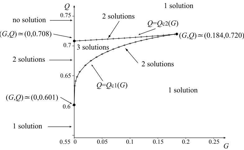
Figure 2 shows a typical G–Q parameter plane showing the number of steady solutions
in the different regions when b = 1, p∞L =p∞R and S = 1. A somewhat similar parameter
plane was recently obtained by Quintans Carou et al. [10, Figure 5] for a closely related “drag
in” problem of a thin film of fluid on a horizontal substrate moving parallel to itself towards
and under a fixed blade. If G = 0 then there is a unique solution for values of Q lying in
the interval 0 < Q ≤ Qc1(0), where Qc1(0) ' 0.601, there are two solutions for values of
Q lying in the interval Qc1(0) < Q < Qc2(0), where Qc2(0) ' 0.708, there is one solution
when Q = Qc2(0), and there is no solution for values of Q satisfying Q > Qc2(0). These
results are consistent with those of Moriarty and Terrill [5]. If G 6= 0 then there are two
possibilities. On the one hand, if 0< G < Gc, where Gc '0.184, then there are either one,
two or three solutions, depending on the value of Q; specifically, there exist critical values
of the flux Qc1 =Qc1(G) and Qc2 = Qc2(G) such that there is a unique solution for values
of Qlying in the interval 0< Q < Qc1(G), there are two solutions when Q=Qc1(G), there
are three solutions for values ofQlying in the interval Qc1(G)< Q < Qc2(G), there are two
solutions when Q =Qc2(G), and there is again a unique solution for values of Q satisfying
Q > Qc2(G). On the other hand, if G≥Gc then there is a unique solution for all values of
Q. Note that, as Figure 2 shows, Qc1(Gc) =Qc2(Gc) =Qc '0.720. Furthermore, Figure 2
also shows that when either G is sufficiently large (specifically when G ≥ Gc) and/or Q is
sufficiently large (specifically when Q ≥ Qc) there is always a unique solution. Note that
when multiple solutions occur they are identical under and downstream of the blade, but
differ upstream of it.
The difference in the (non-dimensional) mass per unit width between the film upstream
of the blade and a uniform film of thickness Q, that is,
∆M =
Z 0
−∞
(h−Q) dx, (30)
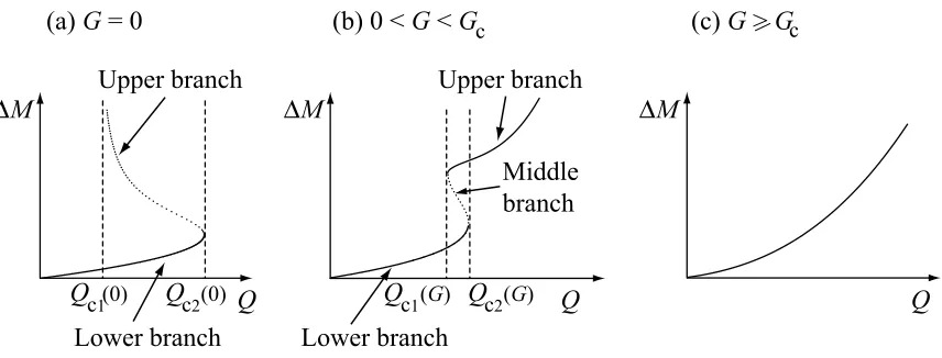
steady solutions. Figure 3 shows sketches of ∆M as a function ofQ forG= 0, 0< G < Gc
and G ≥ Gc, and again illustrates that the number of solutions that exist depends on the
values ofGand Q. The stability results included in Figure 3 are discussed in subsection 2.3
below.
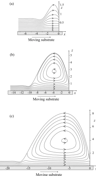
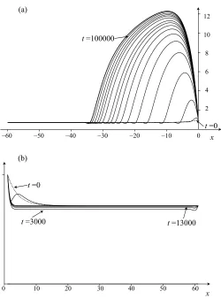
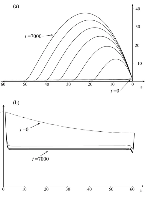
Figures 4 and 5 show the free surface profiles and streamline patterns upstream and
downstream of the blade, respectively, when b = 1, p∞L = p∞R, S = 1, G = 0.1 and Q =
0.705, parameter values for which there are three solutions. The solutions in Figures 4(a),
(b) and (c) lie on the lower, middle and upper branches in Figure 3(b), respectively. In
particular, Figure 4 shows that for these particular parameter values, there is no reverse
flow for the solution on the lower branch, whereas for the solutions on the middle and upper
branches there is a region of reverse flow when h > 3Q = 2.115. Figure 5 shows that for
these particular parameter values there is no reverse flow downstream of the blade.
The solutions in the asymptotic limits Q → 0, Q → ∞, G → 0 and G → ∞ are of
particular interest (not least because they are difficult to calculate numerically) and will
be described in detail in sections 3−5 below, respectively. However, before determining
the solutions in these asymptotic limits we investigate the stability of the steady solutions
described above in the next subsection.
2.3
Stability of the steady solutions
The typical characteristics of most coating processes (such as high speed operation,
non-Newtonian fluids, external pollutants, contaminants in the coating fluid or on the substrate,
machine vibrations or extreme temperatures) mean that they are typically subject to various
instabilities, such as “ribbing” and “fingering” (see, for example, Ruschak [1] and Kistler and
Schweizer [2]).
A linear stability analysis using the standard approach pioneered by Troian et al. [12]
and used extensively by many other authors for a wide range of thin-film flows (see, for
example, Kondic [13]) described by Quintans Carou [11] strongly suggests that solutions on
the upper branch in Figure 3(a) and the middle branch in Figure 3(b) are linearly unstable,
but that solutions on the other branches in Figure 3 are linearly stable. As Quintans Carou
pressure disturbance on a thin film on an inclined plane performed by Kriegsmann et al.
[14]. In particular, the stability of solutions on an infinite domain (as opposed to the
large-but-finite domains used in the numerical calculations) remains open. Quintans Carou [11]
also examined both the energy and the rate of dissipation of the steady solutions, but the
results were inconclusive and so are not discussed any further here.
Support for the linear stability results in the special case of two-dimensional perturbations
can be obtained by calculating the nonlinear temporal evolution of the unsteady (but still
two-dimensional) version of the present problem (for which, of course, the flux no longer
takes a constant value) by solving
ht +
"
h3
3 (Shxx−Gh)x+h
#
x
= 0, (31)
where time t has been non-dimensionalised with L/U, subject to the boundary conditions
(7), (8), (13), (29) and continuity of flux in the x-direction at the ends of the blade. These
calculations were undertaken using a finite-element method implemented via the
MATLAB-based numerical analysis package FEMLAB (now called COMSOL) [15], using the static
solution when the substrate is at rest (i.e. when U = 0) as the initial condition at t = 0.
When G= 0 this initial condition is given by
h=
b0+
(b0−Q) L2
d
x(x+ 2Ld) for −Ld ≤x≤0,
b1+
(b1−Q) L2
d
(x−1)(x−1−2Ld) for 1≤x≤1 +Ld,
(32)
whereLdis the length of the computational domain upstream and downstream of the blade,
and whenG6= 0 it is given by
h=
Q+ (b0 −Q) exp
s G Sx
for −Ld≤x≤0, Q+ (b1 −Q) exp
−
s
G
S(x−1)
for 1 ≤x≤1 +Ld.
(33)
The substrate was started impulsively at t= 0 with constant (nondimensional) speed unity
and the subsequent evolution determined. The results of these unsteady calculations are
entirely consistent with those of the linear stability analysis. For example, on the one hand,
Qc2(G) ' 0.714 from the static solution (shown with a dashed line) towards the unique
steady solution on the upper branch in Figure 3(b) (shown with a thick line). On the other
hand, Figure 7 shows the evolution in a case whenG = 0 and Q= 0.715 > Qc2(0) ' 0.708
from the static solution (again shown with a dashed line). In this case there is no steady
solution and the thickness of the film upstream of the blade increases without bound while
the thickness of the film downstream of the blade decreases with t. In all the stable cases
investigated the free surface evolved from the static solution towards the lowest branch
solution (i.e. the solution with the lowest value of ∆M) available.
3
Solution in the limit
Q
→
0
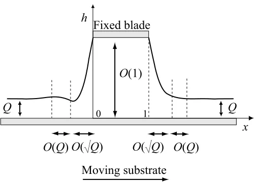
In this section we study the solution in the asymptotic limit of small flux, i.e. in the limit
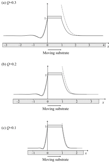
Q→0, in which the film is thin and flat except near to the ends of the blade where a narrow
“meniscus” forms. In the limit Q→ 0 the solutions both upstream and downstream of the
blade have three asymptotic regions: an “outer” region away from the blade in which the
thickness of the film isO(Q) and a narrow “inner” region near the blade of width O(√Q) in
which the thickness of the film is O(1), connected via an even narrower “transition” region
of widthO(Q) in which the thickness of the film rapidly adjusts from its O(Q) outer values
to itsO(1) inner values. The form of the asymptotic solution in the limitQ→0 is sketched
in Figure 8.
In the upstream transition region gravity is negligible. Writing
x=−x0+Qx,ˆ h=Qˆh, (34)
wherex=−x0 is the unknown leading order position of the upstream transition region, we
find that at leading order equation (27) reduces to the well-known Landau–Levich equation
(see, for example, Landau and Levich [16] and Tuck and Schwartz [17]) given by
Sˆhxˆxˆxˆ =
3(1−ˆh) ˆ
h3 , (35)
which must be solved numerically subject to the appropriate matching conditions with the
The appropriate behaviour of ˆh as ˆx→ ∞ is
ˆ
h∼ c0
2 xˆ
2
, (36)
wherec0 is an unknown constant, and ˆh approaches unity in an oscillatory manner as ˆx→
−∞according to
ˆ
h−1∝exp
1 2 3 S 1 3 ˆ x cos √ 3 2 3 S 1 3 ˆ
x+φ
, (37)
whereφ is an unknown phase shift (see, for example, Tuck and Schwartz [17]).
In the upstream inner region near x= 0 surface tension is dominant. Writing
x=qQx,˜ h= ˜h, (38)
we find that at leading order equation (27) reduces to simply
˜
hx˜x˜x˜ = 0, (39)
which can be solved explicitly subject to the appropriate matching conditions with the
upstream transition solution at x = −x0 = −
√
Qx˜0, i.e. ˜h(−x˜0) = 0, ˜hx˜(−x˜0) = 0 and
˜
h˜xx˜(−x˜0) =c0, to yield the leading order upstream inner solution, namely
˜
h= c0
2 (˜x+ ˜x0)
2
. (40)
Since ˜h(0) =b0 we find that x0 is given by
x0 =
s
2b0Q c0
. (41)
As Quintans Carou [11] describes, similar arguments apply downstream of the blade.
Writing
x=x1+Qx,ˆ h=Qˆh, (42)
where x = x1 is the unknown leading order position of the downstream transition region,
the appropriate behaviour of ˆh in the downstream transition region as ˆx→ −∞is
ˆ
h∼ c1
2 xˆ
2
where (unlike in the upstream transition region) the value of the constant c1 can be
deter-mined by solving the Landau–Levich equation (35) numerically, and ˆh approaches unity in
a monotonic manner as ˆx→+∞ according to
ˆ
h−1∝exp
− 3 S 1 3 ˆ x (44)
(see, for example, Tuck and Schwartz [17]). Proceeding as before we find thatx1 is given by
x1 = 1 +
s
2b1Q c1
. (45)
Finally, imposing the continuity-of-pressure condition (29) determines c0 to be equal to
c1.
The leading order mass difference per unit width ∆M defined by (30) is given by
∆M =
√
Qc0x˜ 3 0
6 =O
q
Q
→0. (46)
A uniformly valid composite leading order asymptotic solution forh is
h=Q×
ˆ
h x+x0 Q
!
for x≤0,
ˆ
h x−x1 Q
!
for x≥1,
(47)
where ˆhis the appropriate solution to the Landau–Levich equation (35) upstream and
down-stream of the blade, respectively. Figure 9 shows the free surface profile h computed
nu-merically (marked with a full line) and the composite leading order asymptotic solution (47)
(marked with a dashed line) whenb = 1,p∞L =p∞R and S =G= 1 for various values of Q.
A uniformly valid composite leading order asymptotic stream function ψ is given by
(26) with h given by the composite leading order asymptotic solution (47). Since reverse
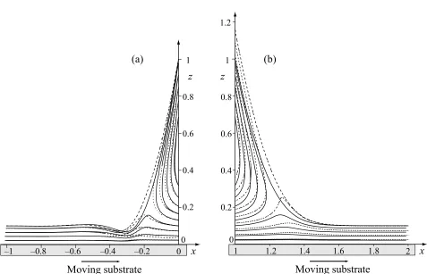
flow occurs when h > 3Q and the thickness of the film is O(1) near the blade, there are
always regions of reverse flow near the ends of the blade in the limit Q → 0. Figure 10
shows streamlines computed numerically (marked with full lines) and using the composite
leading order asymptotic solution (47) (marked with dashed lines) whenb = 1, p∞L =p∞R,
4
Solution in the limit
Q
→ ∞
In this section we study the solution in the asymptotic limit of large flux, i.e. in the limit
Q → ∞, in which there is a large “pile up” of fluid upstream of the blade. In the limit
Q→ ∞ the solution upstream of the blade has three asymptotic regions: an “outer” region
away from the blade of widthO(Q3
) in which the thickness of the film isO(Q) and a narrow
“inner” region near the blade of width O(1/√Q) in which the thickness of the film is O(1),
connected via a “transition” region of width O(1) in which the thickness of the film adjusts
from itsO(Q) outer values to itsO(1) inner values. Downstream of the blade there are only
two asymptotic regions: an “outer” region in which the thickness of the film is O(Q) and a
narrow “inner” region near the blade of width O(1/√Q) in which the thickness of the film
isO(1). The form of the asymptotic solution in the limit Q→ ∞ is sketched in Figure 11.
In the upstream outer region surface tension is negligible. Writing
x=Q3
ˆ
x, h=Qˆh, (48)
we find that at leading order equation (27) reduces to
−Ghˆxˆ =
3(1−ˆh) ˆ
h3 , (49)
and hence the leading order upstream outer solution is given implicitly by
ˆ
h3
3 + ˆ
h2
2 + ˆh+ log(ˆh−1) = 3
G(ˆx+ ˆx0), (50)
and hence the unknown constant ˆx0 is given in terms of ˆh(0) by
ˆ
x0 = G
3
(ˆ
h(0)3
3 +
ˆ
h(0)2
2 + ˆh(0) + log[ˆh(0)−1]
)
. (51)
In the transition region surface tension and gravity are dominant. Writing
x= ˜x, h=Qh,˜ (52)
we find that at leading order equation (27) reduces to
which can be solved explicitly subject to the appropriate matching conditions with the
upstream inner solution at ˜x = 0, i.e. ˜h(0) = 0, and with the upstream outer solution as
˜
x→ −∞, i.e. ˜h→ˆh(0) as ˜x→ −∞, to yield the leading order transition solution, namely
˜
h= ˆh(0)
1−exp
s
G Sx˜
. (54)
The transition solution (54) does not satisfy the correct boundary condition at the left
hand end of the blade, and this is achieved via the upstream inner region in which surface
tension is dominant. Writing
x= √x¯
Q, h= ¯h, (55)
we find that at leading order equation (27) reduces to simply
¯
hx¯x¯x¯ = 0, (56)
which can be solved explicitly subject to the boundary condition ¯h(0) =b0 and the
appropri-ate matching condition with the transition solution as ¯x→ −∞. However, the leading order
value ofhxx is constant throughout the inner region, and so it is not necessary to calculate this
solution in order to determine the leading order contribution to the continuity-of-pressure
condition (29) from the upstream flow; therefore we do not consider it any further here.
In the downstream outer region surface tension and gravity are dominant everywhere.
Writing
x= 1 + ˆx, h=Qˆh, (57)
we find that at leading order equation (27) reduces to
(Shˆxˆˆx−Ghˆ)xˆ = 0, (58)
which can be solved explicitly subject to the appropriate matching conditions with the
downstream inner solution at ˆx = 0, i.e. ˆh(0) = 0, and with the uniform film as ˆx → ∞,
i.e. ˆh→1 as ˆx→ ∞, to yield the leading order downstream outer solution, namely
ˆ
h= 1−exp
−
s
G Sxˆ
. (59)
The downstream outer solution (59) does not satisfy the correct boundary condition at
which surface tension is dominant. However, as for the upstream inner region, it is not
necessary to calculate this solution in order to determine the leading order contribution to
the continuity-of-pressure condition (29) from the downstream flow.
Finally, imposing the continuity-of-pressure condition (29) determines ˆh(0) to be
ˆ
h(0) = 1 + 12I3(1)
G , (60)
where ˆh is given implicitly by (50) and I3(1) is given by (18).
The leading order mass difference per unit width ∆M defined by (30) is given by
∆M = GQ
4hˆ h(0)4
−1i
12 =O
Q4
→ ∞. (61)
A composite leading order asymptotic solution forh (uniformly valid everywhere except
in the inner regions) is
h=Q×
ˆ h x Q3 !
−ˆh(0) exp
s G Sx
for x≤0,
1−exp
−
s
G
S(x−1)
for x≥1,
(62)
where ˆh is given implicitly by (50) and ˆh(0) is given by (60). Figures 12 and 13 show
the upstream and downstream free surface profiles h, respectively, computed numerically
(marked with a full line) and the composite leading order asymptotic solution (62) (marked
with a dashed line)p∞L =p∞R and S =G= 1 for various values ofQ for b = 2 and b = 1,
respectively.
In the upstream outer region the leading order outer stream function ˆψ is
ˆ
ψ = 3
ˆ
h−1 2ˆh3
ˆ
z3
3 −ˆhzˆ
2
!
+ ˆz, (63)
where z =Qzˆ, ψ =Qψˆ, and ˆh is given implicitly by (50). From (63) we see that u = 0 on
the curve ˆz = ˆz0, where ˆz0 is given by
ˆ
z0
ˆ
h = 1−
v u u u t
3−ˆh
thus there is a region of reverse flow between ˆz = ˆz0and the free surface ˆz = ˆhwhen ˆh(0)>3,
and the leading order circulation within the eddy that occurs is equal toQ( ˆψmax−1), where
ˆ
ψmax= ˆψ(0,zˆ0), i.e.
Qhˆh(0)−3i 3
v u u u t
ˆ
h(0)−3
3hˆh(0)−1i =O(Q)→ ∞. (65) A leading order asymptotic stream functionψ (uniformly valid everywhere except in the
inner regions) is given by (26) withhgiven by the composite leading order asymptotic
solu-tion (62). Figures 14 and 15 show the upstream and downstream streamlines, respectively,
computed numerically (marked with full lines) and using the composite leading order
asymp-totic solution (62) (marked with dashed lines) when p∞L =p∞R, S =G= 1 and Q = 3 for
b = 1.5 (for which there is reverse flow) and b = 2 (for which there is no reverse flow), and
forb = 1, respectively.
5
Solution in the limit
G
→
0
In this section we study the upper-branch solution in the asymptotic limit of weak gravity
effects, i.e. in the limit G → 0, in which there is a large “pile up” of fluid upstream of the
blade. (Note that in this limit the middle- and lower-branch solutions simply approach the
upper- and lower-branch solutions in the case G= 0, and so are not considered any further
here.) In the limitG→0 the solution upstream of the blade has five asymptotic regions: an
“outer outer” region far from the blade in which the thickness of the film isO(1), an “outer”
region of widthO(1/G2
) in which the thickness of the film isO(1/G), and an “inner” region
near the blade of width O(1) in which the thickness of the film is O(1), connected via an
“outer transition” region of width O(1/√G) in which the thickness of the film adjusts from
itsO(1) outer outer values to its O(1/G) outer values and an “inner transition” region also
of width O(1/√G) in which the thickness of the film adjusts from its O(1/G) outer values
to its O(1) inner values. Downstream of the blade there is only one region, in which the
thickness of the film is O(1). The form of the asymptotic solution in the limit G → 0 is
In the upstream outer region gravity and viscous shear are dominant. Writing
x= xˆ
G2, h=
ˆ
h
G, (66)
we find that at leading order equation (27) reduces to
ˆ
hxˆ =
3 ˆ
h2, (67)
which can be solved explicitly subject to the appropriate matching condition with the outer
transition solution at x= −x0 = −xˆ0/G2, i.e. ˆh(−xˆ0) = 0, where x =−x0 is the unknown
leading order position of the outer transition region, to yield the leading order upstream
outer solution, namely
ˆ
h = [9(ˆx+ ˆx0)] 1/3
. (68)
In the outer transition region near x = −x0 surface tension, gravity and viscous shear
are all significant. Writing
x=−x0 +
¯
x
√
G, h=
¯
h
√
G, (69)
we find that at leading order equation (27) reduces to
(Sh¯¯x¯x−h¯)x¯ =−
3 ¯
h2, (70)
which must, in general, be solved numerically. The solution of (70) will match with the
leading order outer solution ˆh given by (68) as ¯x → ∞, but not with the uniform film
h = Q as ¯x → −∞, and so this latter matching is achieved in the outer outer region in
which gravity is negligible and at leading order (27) reduces to the Landau–Levich equation.
However, since neither the outer transition region nor this outer outer region feed back any
information to the outer solution, we do not need to consider them any further here.
In the inner transition region surface tension and gravity are dominant. Writing
x= √x˜
G, h=
˜
h
G, (71)
we find that at leading order equation (27) reduces to
which can be solved explicitly subject to the appropriate matching conditions with the inner
solution at ˜x = 0, i.e. ˜h(0) = 0, and with the outer solution as ˜x → −∞, i.e. ˜h → ˆh(0) =
(9ˆx0)1/3 as ˜x→ −∞, to yield the leading order inner transition solution,
˜
h= (9ˆx0) 1/3
1−exp
s
1
Sx˜
. (73)
The transition solution (73) does not satisfy the correct boundary condition at the left
hand end of the blade, and this is achieved via the inner region in which surface tension is
dominant. However, just like in the limit Q → ∞, the value of hxx is constant over this
region, and so it is not necessary to calculate this solution in order to determine the leading
order contribution to the continuity-of-pressure condition (29) from the upstream flow.
Downstream of the blade gravity is negligible everywhere. Writing
x= 1 + ˆx, h= ˆh, (74)
we find that at leading order equation (27) reduces to the Landau–Levich equation given by
Sˆhxˆxˆˆx=
3(Q−ˆh) ˆ
h3 , (75)
which must be solved numerically subject to the boundary condition ˆh(0) = b1 and the
appropriate matching condition with the uniform film as ˆx→ ∞, i.e. ˆh →Q as ˆx→ ∞.
Finally, imposing the continuity-of-pressure condition (29) determines ˆx0 to be
ˆ
x0 =
1
9[−6I2(1) + 12QI3(1)−Shxx(1) +p∞R −p∞L]
3
, (76)
wherehxx(1) is obtained by solving the Landau–Levich equation (75) numerically.
The leading order mass difference per unit width ∆M defined by (30) is given
∆M = (3
5
ˆ
x4 0)
1/3
4G3 =O
1
G3
→ ∞. (77)
A composite leading order asymptotic solution for h (uniformly valid in the upstream
outer and inner transition regions and everywhere downstream of the blade) is
h= "
9(x+x0) G
#1/3
−
9x
0 G
1/3
exp s G Sx
for x≤0,
ˆ
h(x−1) for x≥1,
where x0 = ˆx0/G2, with ˆx0 given by (76), and ˆh is the solution of (75). Figures 17 and 18
show the upstream and downstream free surface profileh, respectively, computed numerically
(marked with a full line) and the composite leading order asymptotic solution (78) (marked
with a dashed line) when b= 1, p∞L =p∞R,S = 1 and Q= 0.9 for various values ofG.
In the upstream outer region the leading order outer stream function ˆψ is
ˆ
ψ = 3
2ˆh2
ˆ
z3
3 −ˆhzˆ
2
!
+ ˆz, (79)
where z = ˆz/G, ψ = ˆψ/G, and ˆh is given by (68). Note that at leading order in this
particular limit ˆψ(ˆz = ˆh) = 0. From (79) we see thatu= 0 on the curve ˆz = ˆz0, where ˆz0 is
given by
ˆ
z0
ˆ
h = 1−
1
√
3; (80)
thus there is always a region of reverse flow between ˆz = ˆz0 and the free surface ˆz = ˆh,
and the leading order circulation within the eddy that occurs is equal to ˆψmax/G, where
ˆ
ψmax= ˆψ(0,zˆ0), i.e.
ˆ
h(0) 3√3G =
(9ˆx0)1/3
3√3G =O
1
G
→ ∞. (81)
A leading order asymptotic stream function ψ (uniformly valid in the upstream outer
and inner transition regions and everywhere downstream of the blade) is given by (26)
with h given by the composite leading order asymptotic solution (78). Figure 19 shows
streamlines computed numerically (marked with full lines) and using the composite leading
order asymptotic solution (78) (marked with dashed lines) when b = 1, p∞L =p∞R, S = 1,
G= 0.2 and Q= 0.9. In particular, Figure 19(b) shows that the convergence of the exact
to the asymptotic solution downstream of the blade as G → 0 is so rapid that they are
indistinguishable for these parameter values.
6
Solution in the limit
G
→ ∞
In this section we study the solution in the asymptotic limit of strong gravity effects, i.e. in
the limitG→ ∞, in which the film is flat except near to the ends of the blade where a narrow
blade have two asymptotic regions: an “outer” region in which the thickness of the film is
O(1) and a narrow “inner” region near the blade of widthO(1/√G) in which the thickness of
the film rapidly adjusts from itsO(1) value at the end of the blade to itsO(1) outer values.
The form of the asymptotic solution in the limit G→ ∞ is sketched in Figure 20.
In the upstream inner region surface tension and gravity are dominant. Writing
x= √xˆ
G, h= ˆh, (82)
we find that at leading order equation (27) reduces to
(Shˆxˆxˆ−hˆ)xˆ = 0, (83)
which can be solved explicitly subject to the boundary condition ˆh(0) = b0 and the
appro-priate matching condition with the upstream outer solution as ˆx → −∞, i.e. ˆh → Q as
ˆ
x→ −∞, to yield the leading order upstream inner solution, namely
ˆ
h=Q+ (b0−Q) exp
s
1
Sxˆ
. (84)
As Quintans Carou [11] describes, similar arguments apply downstream of the blade,
where the leading order inner solution is
ˆ
h=Q+ (b1 −Q) exp
−
s
1
Sxˆ
. (85)
Note that imposing the continuity-of-pressure condition (29) yields no new information
at leading order, and that (84) and (85) coincide with the static solution when the substrate
is at rest in the case G6= 0 given by (33).
The leading order mass difference per unit width ∆M defined by (30) is given by
∆M =
s
S
G(b0 −Q) =O
1
√
G
!
→0. (86)
Figures 21 and 22 show the free surface profile hupstream and downstream of the blade,
respectively, computed numerically (marked with a full line) and the leading order asymptotic
solution (33) (marked with a dashed line) when b = 1, p∞L =p∞R, S = 1 and Q= 0.7 for
A uniformly valid leading order asymptotic stream function ψ is given by (26) with h
given by the leading order asymptotic solution (33). Figures 23 and 24 show the streamlines
upstream and downstream of the blade, respectively, computed numerically (marked with
full lines) and using the leading order asymptotic solution (33) (marked with dashed lines)
when b = 1, p∞L = p∞R, S = 1 and G = 50 (upstream) and G = 5 (downstream) for (a)
Q = 0.3 (for which there is reverse flow when h > 3Q = 0.9) and (b) Q = 0.7 (for which
there is no reverse flow).
7
Conclusions
In the present paper we analysed a simple model of the blade-coating process consisting of
the flow of a thin film of Newtonian fluid on a horizontal substrate moving parallel to itself
with constant speed under a fixed blade of finite length in which the flows upstream and
downstream of the blade are coupled via the flow under the blade.
The appropriate solutions for the fluid velocity and pressure under the blade and both
upstream and downstream of the blade were found explicitly, and the third-order ordinary
differential equation governing the free surface profile (and associated boundary conditions,
one of which couples the solutions upstream and downstream of the blade) was determined.
A combination of asymptotic and numerical methods was used to investigate the number
and nature of the steady solutions that exist. In the absence of gravity we obtained results
that are consistent with those of Moriarty and Terrill [5]. In the presence of gravity we found
that there is always at least one, and (depending on the parameter values) possibly as many
as three, steady solutions, and that when multiple solutions occur they are identical under
and downstream of the blade, but differ upstream of it.
The stability of these steady solutions was investigated numerically. A linear stability
analysis strongly suggests that solutions on the upper branch in Figure 3(a) and the middle
branch in Figure 3(b) are unstable, but that solutions on the other branches in Figure 3
are stable. Support for the linear stability results in the special case of two-dimensional
perturbations was obtained by calculating the nonlinear temporal evolution of the unsteady
cases investigated the free surface evolved from the static solution towards the lowest branch
solution (i.e. the solution with the lowest value of ∆M) available.
The leading order asymptotic behaviour of the steady solutions in the limits of large and
small flux and weak and strong gravity effects, respectively, was examined. These calculations
revealed that in the limitsQ→0 andG→ ∞the film is flat except for a narrow “meniscus”
near to the ends of the blade, while in the limitsQ→ ∞andG→0 there is a large “pile up”
of fluid upsteam of the blade. These calculations also revealed that while regions of reverse
flow (which might be undesirable in practical coating applications) may or may not occur in
the limits Q → ∞ and G → ∞, they always occur both upstream and downstream of the
blade in the limitQ→0 and upstream but not downstream of the blade in the limitG→0.
Furthermore, comparing the exact and asymptotic solutions showed that in most cases the
present asymptotic solutions are practically useful and reasonably accurate approximations
even when the small parameters are not especially small and the large parameters are not
especially large.
Acknowledgements
JQC wishes to thank the University of Strathclyde for financial support via a Graduate
Teaching Assistantship (2002–06) and a Temporary Assistantship (2006–07).
References
[1] Ruschak KJ (1985) Coating flows. Annu Rev Fluid Mech 17:65–89
[2] Kistler SF, Schweizer PM (1997) Liquid film coating. Chapman & Hall, London
[3] European Coating Symposium 2007 website, www.pmmh.espci.fr/~ ecs2007, accessed
on 28th February 2008.
[4] International Coating Science and Technology Symposium website, www.iscst.org,
[5] Moriarty JA, Terrill EL (1996) Mathematical modelling of the motion of hard contact
lenses. Euro J Applied Mathematics 7:575–594
[6] McLeod JB (1996) Solution of a contact lens problem. Euro J Applied Mathematics
7:595–602
[7] Ockendon H, Ockendon JR (1995) Viscous flow. Cambridge University Press, Cambridge
[8] Quintans Carou J, Duffy BR, Mottram NJ, Wilson SK (2006) Shear-driven and
pressure-driven flow of a nematic liquid crystal in a slowly varying channel. Phys Fluids
18(2):027105-1–027105-13
[9] Doedel EJ (1981) AUTO, a program for the automatic bifurcation analysis of autonomous
systems. Cong Numer 30:265–384
[10] Quintans Carou J, Mottram NJ, Wilson SK, Duffy BR (2007) A mathematical model
for blade coating of a nematic liquid crystal. Liq Cryst 34:621–631
[11] Quintans Carou J (2007) Thin-film flow of liquid
crys-tals. PhD thesis, University of Strathclyde. Available online at
www.maths.strath.ac.uk/research/phd mphil theses.
[12] Troian SM, Herbolzheimer E, Safran SA, Joanny JF (1989) Fingering instabilities of
driven spreading films. Europhys Lett 10:25–30
[13] Kondic L (2003) Instabilities in gravity driven flow of thin fluid films. SIAM Review
45:95–115
[14] Kriegsman JJ, Miksis MJ, Vanden-Broeck J-M (1998) Pressure driven disturbances on
a thin viscous film. Phys Fluids 10:1249–1255
[15] COMSOL website, www.comsol.com, accessed on 28th February 2008.
[16] Landau L, Levich VG (1942) Dragging of a liquid by a moving plate. Acta Physicochim
[17] Tuck EO, Schwartz LW (1990) A numerical and asymptotic study of some third-order
or-dinary differential equations relevant to draining and coating flows. SIAM Review 32:453–
B
U
x z
L
z=h(x) z=h(x)
z=b(x)
u w
g
[image:25.612.149.455.251.392.2]Q Q
Figure 1: Steady, two-dimensional flow of a thin film of Newtonian fluid on a horizontal
substrate moving parallel to itself with constant speed U under a fixed blade of finite length
0.6 0.65 0.7
0 0.05 0.1 0.15 0.2
0.75
G Q
1 solution 3 solutions
1 solution
1 solution 2 solutions
no solution Q=Q
c2(G)
Q=Qc1(G)
0.25 0.55
2 solutions 2 solutions
(G,Q)x(0.184,0.720)
[image:26.612.106.499.207.449.2](G,Q)x(0,0.601) (G,Q)x(0,0.708)
Figure 2: Typical G–Q parameter plane showing the number of steady solutions in the
different regions when b = 1, p∞L = p∞R and S = 1. The crosses indicate numerically
(a) G = 0 (b) 0 < G < G (c) G > G
Q (0) Q (0) Q Q Q
Upper branch
Middle branch
Lower branch
∆M ∆M ∆M
c2
c1 Q c1(G) Qc 2(G)
c c
Upper branch
[image:27.612.90.518.238.401.2]Lower branch
Figure 3: Sketches of the mass difference per unit width ∆M given by (30) as a function
of Q, showing the existence of either none, one, two or three solutions, depending on the
values ofGand Q. Linearly stable branches are shown with a full line and linearly unstable
-6 -4 -2 0
-6 -4 -2 0
Moving substrate
x 1
z 1.5
0.5
(a)
1 z
2 3
(b)
-10
Moving substrate
x
-15 -10 -5 0
2
z
4 6
8
Moving substrate
x
-20
(c)
-8
4 5
[image:28.612.149.456.55.620.2]-14 -12
Figure 4: Upstream streamlines when b = 1, p∞L = p∞R, S = 1, G = 0.1 and Q = 0.705,
5 2
Moving substrate
x
1 3 4
0.2 1
0.8
0.6
0.4
0
[image:29.612.200.402.266.435.2]z
−60 −50 −40 −30 −20 −10 0 2 4 6 8 10 12
x t =0 t =100000
0 10 20 30 40 50 60
1
x t =0
t =3000 t =13000 (a)
[image:30.612.179.429.126.464.2](b)
Figure 6: Evolution from the static solution when the substrate is at rest (a) upstream and
(b) downstream of the blade when b = 1, p∞L = p∞R, S = 1, G = 0.1 and Q = 0.715,
parameter values for which there is one steady solution. Times shown aret= 1000 to 10000
(in steps of 1000), t = 12000 to t = 16000 (in steps of 2000), t = 20000 and t = 100000
upstream of the blade, and t = 1000 to 13000 (in steps of 4000) downstream of the blade.
−60 −50 −40 −30 −20 −10 0 10 20
30 40
x t =0
t =7000
0 10 20 30 40 50 60
1
x t =0
t =7000 (a)
[image:31.612.183.425.145.475.2](b)
Figure 7: Evolution from the static solution when the substrate is at rest (a) upstream and
(b) downstream of the blade when b = 1, p∞L = p∞R, S = 1, G = 0 and Q = 0.715,
parameter values for which there is no steady solution. Times shown are t = 1000 to 7000
(in steps of 1000 upstream of the blade and in steps of 2000 downstream of the blade). The
Moving substrate
x h
Fixed blade
O(Q) O(Q)
Q Q
O(1)
0 1
[image:32.612.177.428.260.440.2]O(1 Q) O(1 Q)
0
–1 1 2
Moving substrate Moving substrate
3
2 4 x
0
–3 –2 –1 1
1 (a) Q=0.3
(b) Q=0.2
(c) Q=0.1
0
–2 –1 1 2 3
Moving substrate
x 1
[image:33.612.126.473.70.591.2]x 1
Figure 9: Free surface profile h computed numerically (marked with a full line) and the
composite leading order asymptotic solution (47) in the limitQ→0 (marked with a dashed
Moving substrate
1.4 1.8
1.2
1 1.6 2 x
Moving substrate
–0.6 –0.2
–0.8
–1 –0.4 0 x
0.2 1
0.8
0.6
0.4
0
0.2 1
0.8
0.6
0.4
0
(a) (b)
1.2
[image:34.612.68.545.169.476.2]z z
Figure 10: Streamlines computed numerically (marked with full lines) and using the
com-posite leading order asymptotic solution (47) in the limitQ→0 (marked with dashed lines)
Fixed blade
Moving substrate
O(1)
O(1)
Q
0 1
x h
Q
O(Q)
O(Q 3)
Qh(0)
O(1/ 1Q) O(1/ 1Q)
[image:35.612.118.486.235.468.2]O(1) O(1)
0 1 2 3 4 5 6 7
–150 –100 –50 x 0
2 4 6 8 10
–300 –200 –100 x
(a) Q=3 (b) Q=4 (c) Q=5
0 2 4 6 8 10 12
–600 –400 –200 x
[image:36.612.107.494.219.425.2]Moving substrate Moving substrate Moving substrate
Figure 12: Upstream free surface profile h computed numerically (marked with a full line)
and the composite leading order asymptotic solution (62) in the limitQ→ ∞(marked with
a dashed line) when b = 2, p∞L = p∞R and S = G = 1 for (a) Q = 3, (b) Q = 4 and (c)
(a) Q=3 (b) Q=4 (c) Q=5
1 2 3
4
5
0
1 2 3 4 5 6 7 8 x
Moving substrate
1 2 3
4
5
0
1 2 3 4 5 6 7 8 x 1 2 3
4
5
0
1 2 3 4 5 6 7 8 x
[image:37.612.104.500.228.412.2]Moving substrate Moving substrate
Figure 13: Downstream free surface profilehcomputed numerically (marked with a full line)
and the composite leading order asymptotic solution (62) in the limitQ→ ∞(marked with
a dashed line) when b = 1, p∞L = p∞R and S = G = 1 for (a) Q = 3, (b) Q = 4 and (c)
0 1 2 3 4 5 6 7 z
–100 –80 –60 –40 –20 x
Moving substrate (b) b=2
0
–500 –400 –300 –200 –100 x
Moving substrate (a) b=1.5
2 4 6
8
[image:38.612.111.490.215.444.2]10 12 z
Figure 14: Upstream streamlines computed numerically (marked with full lines) and using
the composite leading order asymptotic solution (62) in the limit Q → ∞ (marked with
1 2 3 4 5 6 7 8 x
Moving substrate 0
0.5 1 1.5
2 2.5
[image:39.612.194.414.229.428.2]3 z
Figure 15: Downstream streamlines computed numerically (marked with full lines) and
using the composite leading order asymptotic solution (62) in the limit Q → ∞ (marked
Fixed blade
Moving substrate
O(1)
0 1
x h
O(1/G)
O(1/G 2) O(1/ G)
h(0) G o
O(1) O(1)
1
O(1/ 1G) O(1/ 1G)
[image:40.612.111.497.237.469.2]O(1) O(1)
0 2 4 6 8 10
–50 x
2
4 6 8 10 12 14
–100 –50 x 0
5 10 15 20
–200 –100 x
(a) G=0.4 (b) G=0.3 (c) G=0.2
–150
Movingsubstrate
0
[image:41.612.120.483.215.423.2]Movingsubstrate Movingsubstrate
Figure 17: Upstream free surface profile h computed numerically (marked with a full line)
and the composite leading order asymptotic solution (78) in the limit G→0 (marked with
a dashed line) when b= 1, p∞L =p∞R,S = 1 and Q= 0.9 for (a) G= 0.4, (b) G= 0.3 and
(a) G=0.4 (b) G=0.3 (c) G=0.2
0.9 0.92 0.94 0.96 0.98 1
1 2 3 4 5 x
Moving substrate
0.9 0.92 0.94 0.96 0.98 1
1 2 3 4 5 x 1 2 3 4 5 x
0.9 0.92 0.94 0.96 0.98 1
[image:42.612.107.501.224.411.2]Moving substrate Moving substrate
Figure 18: Downstream free surface profilehcomputed numerically (marked with a full line)
and the composite leading order asymptotic solution (78) in the limit G→0 (marked with
a dashed line) when b = 1, p∞L = p∞R, S = 1 and Q = 0.9 for (a) G = 0.4, (b) G = 0.3,
5 10 15 20
z
–300 –250–200–150 –100 –50 0 x
Moving substrate
0 0.2 0.4 0.6 0.8 1
z
1 2 3 4 5 6 7 x
Moving substrate 0
[image:43.612.121.485.218.454.2](a) (b)
Figure 19: Streamlines computed numerically (marked with full lines) and using the
com-posite leading order asymptotic solution (78) in the limitG→0 (marked with dashed lines)
when b = 1,p∞L =p∞R, S = 1, G= 0.2 and Q= 0.9. The exact and asymptotic solutions
Fixed blade
Moving substrate
O(1)
0 1
x h
O(1)
[image:44.612.191.412.282.422.2]O(1/ 1G) O(1/ 1G)
(a) G=10 (b)G=50 (c)G=100
0.7
0.75
0.8
0.85
0.9
1
-8 -4 -2 x
Movingsubstrate 0.95
-6
Movingsubstrate Movingsubstrate 0.7
0.75
0.8
0.85
0.9
1
0.95
-20 -15 -10 -5 x
0 0 -25 -20 -15 -10 -5 0 x
0.7
0.75
0.8
0.85
0.9
1
[image:45.612.95.508.225.414.2]0.95
Figure 21: Upstream free surface profile h computed numerically (marked with a full line)
and the leading order asymptotic solution (33) in the limit G→ ∞ (marked with a dashed
line) when b = 1, p∞L = p∞R, S = 1 and Q = 0.7 for (a) G = 10, (b) G = 50 and (c)
(a) G=2 (b)G=5 (c)G=10
0.7 0.75 0.8 0.85 0.9 1
1 2 2.5 x
Movingsubstrate 0.95
1.5 1 2 2.5 x
Movingsubstrate 1.5
0.7 0.75 0.8 0.85 0.9 1
0.95
0.7 0.75 0.8 0.85 0.9 1
0.95
1 2 2.5 x
[image:46.612.98.508.225.434.2]Movingsubstrate 1.5
Figure 22: Downstream free surface profilehcomputed numerically (marked with a full line)
and the leading order asymptotic solution (33) in the limit G→ ∞ (marked with a dashed
x
Moving substrate
(a) Q=0.3 (b) Q=0.7
0.2
0.4
0.6
0.8 1
z
0 0
–2.5 –2 –1.5 –1 –0.5
Moving substrate
0.2
0.4
0.6
0.8 1
z
0
[image:47.612.100.504.218.436.2]–3.5 –3 x –10 –5 0
Figure 23: Upstream streamlines computed numerically (marked with full lines) and using
the leading order asymptotic solution (33) in the limit G→ ∞ (marked with dashed lines)
(a) Q=0.3 (b) Q=0.7
2 2.5 3 3.5 4
Movingsubstrate
0.2 0.4 0.6 0.8 1
z
0
1 1.5 x 2 2.5 3 3.5 4
Movingsubstrate
0.2 0.4 0.6 0.8 1
z
0
[image:48.612.113.494.204.452.2]1 1.5 x
Figure 24: Downstream streamlines computed numerically (marked with full lines) and using
the leading order asymptotic solution (33) in the limit G→ ∞ (marked with dashed lines)