City, University of London Institutional Repository
Citation:
Ma, Q. & Zhou, J. (2009). MLPG_R Method for Numerical Simulation of 2D
Breaking Waves. CMES: Computer Modeling in Engineering & Sciences, 43(3), pp. 277-304.
doi: 10.3970/cmes.2009.043.277
This is the accepted version of the paper.
This version of the publication may differ from the final published
version.
Permanent repository link:
http://openaccess.city.ac.uk/13214/
Link to published version:
http://dx.doi.org/10.3970/cmes.2009.043.277
Copyright and reuse: City Research Online aims to make research
outputs of City, University of London available to a wider audience.
Copyright and Moral Rights remain with the author(s) and/or copyright
holders. URLs from City Research Online may be freely distributed and
linked to.
City Research Online:
http://openaccess.city.ac.uk/
[email protected]
MLPG_R Method for Numerical Simulation of 2D Breaking Waves
Q.W. Ma1, 2 and J.T. Zhou1
Abstract: Following our previous work, the Meshless Local Petrov-Galerin method based on Rankine source solution (MLPG_R) will be extended in this paper to deal with breaking waves. For this purpose, the governing equation for pressure is improved and a new technique called Mixed Particle Number Density and Auxiliary Function Method (MPAM) is suggested for identifying the free surface particles. Due to complexity of the problem, two dimensional (2D) breaking waves are only concerned here. Various cases are investigated and some numerical results are compared with experimental data available in literature to show the newly developed method is robust.
1
Key words: MLPG_R method; Mixed Particle Number Density and Auxiliary Function Method (MPAM); breaking waves; solitary wave.
1 Introduction
Wave breaking plays a significant role in air–sea interactions, such as energy and momentum transfer from wind to water and from waves to currents, and in the generation of turbulence in the upper ocean. It also plays an important role in bed-sea interactions, such as sediment transport or sand bar formation. In addition, wave breaking is the most concerned phenomenon associated with wave-structure interaction, for instance, interactions of breaking waves with breakwaters, offshore wind energy structures, offshore oil and gas exploitation platforms and transport vehicles. The force produced by these interactions is an important factor which must be considered in engineering design to secure the safety of the structures. As a result, wave breaking has been a topic of prime importance to the coastal/offshore engineering and environmental communities for many years. Nevertheless, it still remains a great challenge due to its high nonlinearity and complexities.
Some investigations have been carried out by the laboratory experiments or field observations [Bonmarin, (1989); Rapp and Melville, (1990); Li and Raichlen, (2003)]. These investigations produced very useful results for some cases but are generally very expensive. In addition, many studies are based on numerical analysis, for which various numerical methods have been developed. The numerical methods can be grouped into mesh-based methods and meshless methods. The mesh-based methods for steep and/or breaking waves mainly include the finite difference method [e.g, Miyata,
1School of Engineering and Mathematical Sciences City University London, Northampton Square, London, UK, EC1V 0HB;
2Communication: [email protected]
(1986); Lin and Liu, (1998)]; finite element method [e.g, Ma and Yan, (2006)], boundary element method [e.g, Grilli, Guyenne and Dias, (2001)] and finite volume method [e.g, Greaves (2009); Klessfsman, Fekken, Veldman, Iwanowski, Buchner (2005); Devrard, Marcer, Grilli, Fraunie and Rey, (2005]]. They all produced many impressive results. However, a limitation of mesh-based methods is that a computational mesh/grid is required and needs to be managed. Depending on whether using Lagrangian or Eulerian formulation, the mesh/grid may need to be updated repeatedly or to be refined to follow the motion of the free surface and need to be maintained to have good quality. This is often a difficult or time-consuming task, particularly in the cases with breaking waves.
Alternatives are meshless methods. In these methods, the fluid domain is discretised as nodes or particles, instead of a computational mesh/grid. Therefore, the limitation associated with mesh does not exist. So far, many meshless methods have been developed and reported in literatures, such as the Moving Particle Semi-implicit method (MPS) [e.g, Koshizuka and Oka, (1996); Gotoh and Sakai (2006); Khayyer and Gotoh (2008)], the Smooth Particle Hydrodynamic method (SPH) [e.g, Monaghan (1994); Khayyer, Gotoh and Shao (2008)], the finite point method [e.g, Onate, Idelsohn, Zienkiewicz, Taylor and Sacco (1996)], the element free Galerkin method [e.g, Belytschko, Lu and Gu (1994)], the diffusion element method [e.g, Nayroles, Touzot and Vilon (1992)], the method of fundamental solution [e.g, Wu, Tsay, Young (2006)] and so on. Among them, the MPS and SPH have been used to simulate breaking wave problems. For example, Monaghan (1994) modelled waves propagating over beaches; Lo and Shao (2002) and Koshizuka and Oka (1996) simulated the collapse of a water column; and Gotoh and Sakai (2006) investigated the breaking waves and the wave-body interaction problems. Khayyer, Gotoh and Shao (2008) simulated the breaking and post-breaking of solitary waves on a slope using the SPH method. Issa, Violeau, Lee and Flament (2009) made a review on how to deal with turbulent models in the SPH method.
bending problems [Atluri and Zhu (2000)], shell and thermal elastic problems [Sladek, Sladek, Wen and Aliabadi (2006), Sladek, Sladek, Zhang and Tan (2006) and Jarak, Soric and Hoster (2007)], three dimensional elasto-static and -dynamic problems [Han and Atluri (2004a,b)], and some fluid dynamic problems, such as steady flow around a cylinder [Atluri and Zhu (1998)], steady convection and diffusion flow [Lin and Atluri (2000)] in one and two dimensions and lid-driven cavity flow in a two dimensional box [Lin and Atluri (2001), Mohammadi (2008)]. Over the past couple of years, the method has been extended to deal with more advanced problems. Han, Liu, Rajendran and Atluri (2006) made an advance in analyzing very complicated high-speed impact, penetration and perforation problems and indicated that the MLPG can be much faster than mesh-based methods for the problems of this kind. Li and Atluri (2008a,b) applied the MLPG method to analyze material orientation and to perform topology optimization of anisotropic solids and structures. Sladek, Sladek, Tan and Atluri (2008) studied transient heat conduction in 3D anisotropic solids. Ching and Chen (2006), Sladek, Sladek, Zhang and Solek (2007), Sladek, Sladek, Solek and Wen (2008), Sladek, Sladek, Solek, Wen and Atluri (2008) dealt with various thermo-structure dynamic problems. Vavourakis, Sellountos and Polyzos, (2006) and Sellountos, Sequeira and Polyzos (2009) performed elastic transient analysis using the MLPG(LBIE) method. Dang and Sankar (2008) applied the MLPG method to micromechanical analysis of periodic composites. Arefmanesh, Najafi and Abdi (2008) considered non-isothermal lid-driven cavity flow and non-non-isothermal flow over an obstacle. Developments are also made in refining the MLPG method, such as Yuan, Chen and Liu (2007), Pini, Mazzia and Sartoretto (2008), Cai and Zhu (2008), Chen, Liu and Cen (2008), Wang, Zhou, Nie and Kong (2008).
In addition to its various applications to solid and general fluid problems, Ma (2005a) extended the MLPG method to simulating nonlinear water waves and produced some encouraging results. In that paper, the simple Heaviside step function was adopted as the test function to formulate the weak form over local sub-domains, resulting in one in terms of pressure gradient.
In Ma (2005b), the MLPG method was further developed into a new form called the MLPG_R method, better suitable for modelling nonlinear water waves. In the MLPG_R method, the solution for Rankine sources rather than the Heaviside step function was taken as the test function. Based on this test function, a weak form of governing equations was derived, which did not contain any gradients of unknown functions and therefore made numerical discretisation of the governing equation relatively easier and more efficient. A semi-analytical technique was also developed to evaluate the domain integral involved in this method, which dramatically reduce the CPU time spent on the numerical evaluation of the integral. Numerical tests showed that the MLPG_R method could be twice as fast as the MLPG method for modelling nonlinear water wave problems.
Ma (2008) made another step forward in the development of the MLPG_R method for water waves. In that paper, a new
meshless interpolation was suggested, which is as accurate as the moving least square method but much more efficient, particularly for computation of gradient of unknown functions.
The MLPG_R method has been applied to model various nonlinear water waves, including the waves generated by a wavemaker, sloshing waves and freak waves [Ma, (2007)]. In this paper, it will be extended to deal with breaking waves. Because breaking waves are more complicated than non-breaking waves, new techniques will be developed to achieve the purpose. Further to them, different configurations under different wave conditions will be considered and some results will be compared with experimental data available in the public domain to show its accuracy.
2 Mathematical formulation
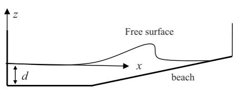
The flow of incompressible fluid is considered, which is confined in a two dimensional (2D) domain, as shown in Fig. 1. The figure also shows the coordinate system, in which the
[image:3.595.307.537.421.508.2]x-axis is on the mean free surface and x=0 corresponds to the left wall unless mentioned otherwise. In some cases, the sloped beach may be considered. For these cases, the left wall will move like a wavemaker to generate waves. d is the mean depth of fluid in the range from the wall to the sloped beach.
Fig. 1 Sketch of the computational domain
The continuity equation and the Navier-Stokes equation (referred as NS equation hereafter) together with proper boundary conditions are given as follows:
0
u& , (1)
u g p Dt
u
D& 1 &Q2&
U , (2)
where g& is the gravitational acceleration; u& is the fluid velocity; U and
Q
are the density and the kinematical viscosity of fluid, respectively; andpis the pressure. On a rigid boundary, the velocity satisfies,U n u
n&& &&, (3)
Free surface
beach
d
z
where n& is the unit normal vector of the rigid boundary and
U& is its velocity. On the free surface, the condition is specified by
0
p . (4)
The mathematical model given by Eqs. (1) to (4) is solved using a time marching procedure, which has been described by our previous papers [e.g, Ma, (2005b)] and will be summarised below.
Suppose the velocity, pressure and the location at nth time step (t=tn) are known, one can use the following procedure to find them at (n+1)th time step.
(1) Calculate the intermediate velocity ( u&* ) and position(r&*) of particles using
t u t g u
u&* &n&' X2&n' , (5)
t u r
r&* &n&*' , (6)
wherer*is the position vector of particles, the superscript n
represents nth time step; 'tis the increment of time step.
(2) Evaluate the pressure pn+1 using the following semi-implicit equation * 2 * 1 1
2 (1 ) u
t t
p
n
n &
' '
DU U D U , (7)
where D is an artificial coefficient between 0 and 1, and
1
n
U and U* are the fluid density at (n+1)th time step and at the intermediate time step, respectively. For the incompressible flow, the density should be a constant and soUn1 = U, where U is the fluid density specified initially. The density U* at the intermediate step may not be the same as U because the velocity and position calculated in Eqs. (5) and (6) do not necessarily satisfy the continuity equation given in Eq. (1).
(3) Calculate the fluid velocity and update the positions of the particles using
1
** 'tpn
u U
& (8)
1 *
** *
1
' n
n p t u u u u U & &
& (9)
t u r
r&n1 &n&n1' (10)
(4) Go to the next time step
The above formulation is different from our previous work by Ma (2005a, b and 2008) in two aspects. (1) The viscous term is considered here but not considered there. (2) There are two terms on the right hand side of Eq. (7) rather than one term in the previous publications. Nevertheless, if
D
0
, the formulation here become the formulation in previouspapers automatically. As pointed out in our cited papers, viscous effect is neglectable if waves are not breaking. That is why the associated term is ignored in those papers that considered only non-breaking steep waves. This paper aims to study breaking waves and thus viscosity is likely important. As a result, we must take it into account in Eq. (2). Regarding the change in Eq. (7), it can be shown that the governing equation for the pressure have two forms: one corresponding to D 0and the other toD 1 [Koshizuka & Oka (1996); Idelsohn Storti and Onate (2001)], and both are derived by applying the continuity equation for incompressible fluid. Without wave breaking, the formulation with D 0 can yield good results as demonstrated in our previous papers. However, when wave breaking occurs, splash and re-entry take place frequently. In such cases, none of the two forms on their own works very well. Assigning a nonzero small value to Dcan improve the results dramatically, which will be demonstrated in the later section of the paper. Such an approach has also been adopted by Zhang, Morita, Kenji and Shirakawa (2006) for the MPS method.
2 MLPG_R formulation
Eq. (7) is solved by using the MLPG_R method. The details of the MLPG_R formulation and other techniques can be found in Ma (2005b). Here, we focus only on the aspects necessary to accommodate the change in Eq. (7). This method is based on a number of nodes or particles, which discretize the computational domain. Some nodes are located on the boundaries and others lie inside the fluid domain. At each of the inner nodes, a sub-domain is specified, which is a circle for 2D cases and Eq. (7), after multiplying by an arbitrary test function M, is integrated over the sub-domain, which becomes:
³
³
: : : ' ' : I I I I n d u t t d p M U D U U D M ] ) 1 ([ 2 *
* 1
2
&
(11)
where :I is the area of the sub-domain (also called integration domain) centered at Particle I and the density
1
n
U has been replaced by Ubased on the discussion after Eq. (7). In the MLPG_R method, the test function is taken as the solution of Rankine source, i.e., the function
M
satisfies0
2
M , in :I except for the center and
M
0
, on w:Iwhich is boundary of :I. The expression of the solution for Rankine source is
) / ln( 2 1 I R r S
M for 2D cases (12)
In Eq. (11), the second derivative of unknown pressure and the gradient of the intermediate velocity are included. Numerical calculation of the derivative and gradient does not only requires much computational time but also degrades the accuracy. In order to obtain a better form, Eq. (11) is changed, by adding a zero term p2M and applying the
Gauss’s theorem, into
³
³
³
³
w : w : w : w : : ' ' : ' H H M U M U D M U U D M M I I I I d u t dS u n t d t dS p n p n ] ) ( )[ 1 ( )] ( ) ( [ * * 2 * & & & & & (13)wherewH is a small surface surrounding the center of :I,
which is a circle in 2D cases. The reason for adding wH is that the test function M in Eq. (11) becomes infinite at r=0 and so the Gauss’s theorem can not be used otherwise. In the same way as in Ma (2005b), Eq. (13) can be reduced to:
: ' '
³
³
: : w d u t R t p dS p n I I I I I M U D U U D M * 2 2 * ) 1 ( 4 ) ( & &, (14)
where it has been assumed that the increment of the density
(
U
U
*) is a constant within the sub-domain and so equal to its value at Particle I, which is acceptable not only because the density should not change much due to the change in the intermediate position of the particle but also because the small error caused due to the assumption is further reduced by multiplying the coefficientD
of a small value. The term may be evaluated in a more accurate way, for example by interpolation as done for the second term but such a way will not improve the accuracy significantly due to the reason. It is obvious that Eq. (14) requires the intermediate density that is not computed in the MLPG_R method. Actually, the density can be replaced by a particle number density (PND) defined by Koshizuka and Oka (1996) in their MPS method as follows:¦
z M I j j I j I W r rn , 1
|)
(| , (15)
where W is a weight function in terms of the distance between Particle I and Particle j, which becomes zero when the distance is larger than a certain value. The domain, within which the weight function is not zero, is called support domain. In the above equation, M is the total number of particles in the support domain of Particle I. As indicated by Koshizuka and Oka (1996), the PND is related to the density by:
³
VII I I I dV r W n m ) (
U , (16)
where mI is the mass of Particle I. After applying Eq. (16),
Eq. (14) becomes
: ' '
³
³
: : w d u t R n n n t p dS p n I I I I M U D U D M * 2 0 * 0 2 ) 1 ( 4 ) ( & & (17)Ma (2005b) has detailed the method to discretise Eq. (17), in which the pressure on the left hand side is interpolated by a moving least square method (MLS) and the integration on the right hand side is evaluated by a semi-analytical technique. So the similar discussion will not be repeated here.
3 Boundary Conditions on a rigid boundary
Eq. (3) gives the condition on a rigid boundary in terms of velocity. To solve the problem about the pressure, the condition in terms of pressure is required on the boundary. For cases without considering the viscosity, the condition [Ma, (2005a, b)] is given as:
¸¹ · ¨©
§
p n g n U
n & & & &
&. U (18a)
whereU
&
is the acceleration of the boundary. This expression can be derived directly from Eqs. (2) and (3) by taking Q 0. WhenQz0 as in the cases considered in this paper, one may also derive the condition by using Eqs. (2) and (3) and obtain:
¸ ¹ · ¨©
§
p n g n U n u
n & &
& & & &
&. U Q 2 . (18b)
It is obvious that one must compute the term 2u& when applying this condition, which needs to estimate the second order derivative at the rigid boundary. Although there is no much difficulty to do so theoretically, the error associated with it is not easy to be suppressed in computational practice as the fluid particles located only on one side of the boundary. Therefore, it is better to avoid the computation of the second order derivative when possible. For this reason, Eqs. (3) and (9) are combined to give an alternative equation for the boundary condition as follows:
)
( * 1
1
'
n n
U u n t p
n* U & & & , (19)
* 1
u n t p
n* n && '
U . (20)
Although one still needs to calculate 2u& , which is inevitable, to estimate u&*, the second order derivative term is not explicitly involved in Eqs. (19) and (20) and does not need to be calculated again after u&* is available. This formulation will be used in this paper.
In numerical discretisation, Eq. (19) is directly applied to the nodes or particles on the rigid boundary, as what we did in Ma (2005b). However, in our previous papers, the gradient of the pressure is approximated by using the MLS. In this paper, it will be evaluated by the simplified finite difference interpolation (SFDI) scheme, recently proposed by Ma (2008). The SFDI scheme is as accurate as the MLS method but need less computational time. The reader is referred to Ma (2008) for more details about the scheme.
4 Technique for identifying free surface particles
In order to find solution for pressure by using the governing equation in previous section, all the particles need to be sorted into three groups: those on rigid boundaries (referred as wall particles), those on the free surface (referred as free surface particles) and others (referred as inner particles). The wall particles are always attached to the rigid boundary in our modeling. Eq. (19) or (20) is applied to wall particles. Eq. (17) is applied to the inner particles. The pressure at the free surface particles is specified by the condition in Eq. (4). For non-breaking waves, one can assume that the particles initially on the free surface remain on the free surface. Therefore, the free surface particles need only to be specified at the first step and there is no need to identify them during the simulation.
However, for the cases with breaking waves as considered in this paper, the fluid particles initially on the free surface may not remain on the free surface during calculation. Actually, the particles initially within the fluid can emerge on the free surface and the particles initially on the free surface can immerge into the inner fluid domain due to wave breaking and splashing. Consequently, it is necessary to identify which particle is on the free surface when modeling breaking-wave cases.
There is a similar requirement on identifying the free surface in mesh-based numerical models for breaking waves. Several methods have been developed in the community using those models, such as level set method and volume-of-fluid technique. A brief review can be found in Greaves (2009).
Nevertheless, the identification of free surface particles remains to be a big challenge in meshless particle modeling, particularly for those of true meshless models without any background mesh, like the MLPG_R method. In the SPH method, the free surface particles are identified by the density; i.e., if the ratio of the density of a particle to the fluid density is less than a specified value, such as 1%, it is then identified
as a free surface particle [e.g., Lo and Shao, (2002)]. The computation of the density in the SPH requires a background mesh, which is not available in the MLPG_R method. Another technique is based on the particle number density suggested for the MPS method by Koshizuka and Oka (1996) and also used by Gotoh and Sakai (2006). This technique uses the following parameter:
0 n nI
I
E , (21)
where
n
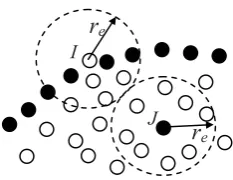
I is the particle number density at Particle I , as defined in Eq. (15), which is computed by using the particle configuration after the motion corresponding to the intermediate velocity. If EI E , Particle I is considered as a free surface particle. This approach is named as Particle Number Density Method, abbreviated to PNDM in this paper. Currently, there is no common agreement about how to specify the value of E. It is problem-dependent. Different researchers use different values. For example, it was 0.97 in Koshizuka and Oka (1996) and Gotoh and Sakai (2006) while it was 0.99 in Shao and Lo (2003). Results look to be promise in all the papers even with different values forE. [image:6.595.360.477.607.697.2]According to our numerical tests, the simple technique is not very robust. There are always many particles that are incorrectly identified (i.e., free surface particles are identified as inner particles or vise versa). The incorrect identification could not be rectified by simply choosing a different value for E. Similar observation has also been described by Lee and Park (2007). To shed some light on the reason for this, let us look at Particle I and J in Fig. 2. Particle I is near the crest of a steep wave. In this area, the particles on the free surface are generally much closer to each other than in other areas and so the particle number density associated with them can be very higher. As a result, Particle I may be incorrectly identified as an inner particle rather than a free surface particle by the above criterion. On the other hand, the neighbor particle of Particle J is quite far from it. The value of the particle number density can be relatively smaller and so it may be incorrectly classified as a free surface particle even though it should be an inner particle. In addition to these situations, two or three splashed particles may be very close to each other and so may also be incorrectly identified as inner particles though they should be considered as free surface particles for the sake of solving pressure.
Fig. 2 Two typical examples of incorrect identification of free surface particles. (Solid circle represents free surface particle identified by the PNDM; hollow ones represent inner
particles identified by the PNDM).
I
r
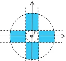
eFig. 3 Local coordinate system at Particle I (inner circle denotes its integration domain; outer circle denotes its
influence domain)
To improve the robustness of identification of free surface particles, a new approach will be suggested here. The approach is based on three auxiliary functions. The first auxiliary function is defined by
¯ ®
t
0 ,
0
1 ,
1 ) ( _
NumA NumA I
a
fsp (22)
whereNumA represents the number of free surface particles existing in the influence domain (Df) of Particle I in previous time step. The second auxiliary function is
¯ ®
d3 ,
0
4 ,
1 ) ( _
NumB NumB I
b
fsp , (23)
whereNumB represents the number of quadrants occupied by the neighbor particles of Particle I in a local coordinate system originating at Particle I, as shown in Fig. 3. The third auxiliary function is given by
¯ ®
d3 ,
0
4 ,
1 ) ( _
NumC NumC I
c
fsp , (24)
whereNumC represents the number of colored (or shaded) rectangles in Fig. 3 in which there is at least one fluid particle. If one of following conditions is met when they are checked sequentially, Particle I is identified as a free surface particle.
(a) no inner particle in Df except for I;
(b) EI 0.97 andfsp_a(I) 1;
(c) EI 0.97, fsp_a(I) 1 and fsp_b(I) 0; (d) EI 0.97, fsp_a(I) 1 and fsp_c(I) 0.
Satisfying the condition (a) indicates that the particle concerned is in the group of particles which belong to the part of splashing fluid. The condition (b) identifies those free surface particles with at least one neighbour particle on the free surface. The condition (c) and (d) picks up those free surface particles with sufficient large number of neighbour particles but with no particle in a sufficient large part of its influence domain. This approach will be called as Mixed
Particle Number Density and Auxiliary Function Method, abbreviated to MPAM.
Using this new approach, the incorrect identification of the free surface particles may be avoided. Lets us look again at Particle I in Fig. 2. There are more than one free surface particle in its influence domain, and a large part of its influence domain is not occupied by any particle. As a result, fsp_a(I) 1, fsp_b(I) 0 and it will be identified, by applying Condition (b) or (c), as a free surface particle no matter what is the value for EI. For Particle J shown in Fig. 2, there are no free surface particles existing in its influence domain and so fsp_a(I) 0 . Therefore, even though
97 . 0
I
E for the particle, no one of four conditions will be met and thus Particle J is not identified as a free-surface particle.
5 Parameter study and validation
In the above formulation, we introduced the parameter D and the new technique to identify the free surface particles. In this section, some numerical results will be first discussed to show the effectiveness of the techniques. After that, validation against experimental data and the investigation on convergent properties will be presented.
In the following cases, water will be used as the fluid and the standard value of water density and viscosity are chosen. In addition, the parameters with a length scale are nondimensionalised by the water depth d and the time is
nondimensionalised by d/g , i.e. t W d/g . In all the
cases, the particles are uniformly distributed at beginning with the same distance between the particles in both directions. The number of particles along z-direction is represented by Nz.
5.1 Effectiveness of Parameter
D
As discussed in the paragraph just after Eq. (10), either of the form of Eq. (7) with D 0or the one withD 1does not work well in the cases for breaking waves. The root cause of the problem, based on the observation of numerical results, is that the distribution of the particles becomes over-distorted. This sub-section will present some results indicating that the problem may be overcome by choosing appropriate value for
D
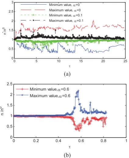
.For this purpose, one needs to define an indicator that reflects the level of distortion of particle distribution. We will choose the PND as the indicator. That is because the change in the PND at inner particles defined in Eq. (15) can reflect the feature of particle distributions. At the beginning, the difference between the largest and the smallest PND of inner particles is a given value depending on the initial distribution of particles. It is very small if the initial distribution is almost uniform. With increase in the level of distortion of particle distribution, the difference between the largest and the smallest PND will grow. The larger the difference, the severer the distortion is.
To show how the PDN changes, a dam breaking problem is considered. This is a classical case for studying violent free surface flow, which has been numerically simulated by many researchers using various methods, such as Monaghan (1994) and Koshizuka and Oka, (1996). The geometry we use here is similar to that in Koshizuka and Oka (1996), i.e., the ratio of the length to the height of the water column confined by a vertical plate is 0.5 with the total length of the tank being 2. The plate is lifted off at =0 instantaneously. To model this case, we take Nz=50 and the time step 'W as 0.004. Because our aim here is to show the effectiveness of D, the change in particle number (Nz) and time step is not considered, though we believe that the values chosen here are sufficient according to our numerical tests given below.
0 5 10 15 20 25
0 0.5 1 1.5 2 2.5 3
W
n
*/n
0
Minimum value, D=0
Maximum value, D=0
Minimum value, D=0.1
Maximum value, D=0.1
(a)
0 0.2 0.4 0.6 0.8 1
0 0.5 1 1.5 2 2.5
W
n
*/n
0
Minimum value,D=0.6
Maximum value,D=0.6
(b)
Fig. 4 Effects of different D on the PND
The time histories of the ratios of the maximum and minimum values of the PND to the initial PND for inner particles excluding the free surface particle are recorded at each intermediate time step. They are plotted in Fig. 4(a) for the cases with D 0 and
D
=0.1. One can see from this figure that the maximum ratio fluctuates at about 1.7 and the minimum ratio change around 0.5 for the case with D 0. The difference between them is about 1.2. On the other hand, the difference between the maximum and minimum ratios for the case with D 0.1is about 0.4 and tends to be consistently smaller with increase of time. The effect of D is further illustrated by using Fig. 5, where the configurations of particles at the same instant for D 0 and D 0.1 are plotted and two small areas are enlarged in the figure. The distribution of the particles in the enlarged areas for D 0.1 is more uniform than that forD 0. These observationsshow that the particle distribution in the case with D 0.1 is better than in the case with D 0and the former is likely to lead to better results.
Fig. 5 (a) D 0.0
Fig. 5 (b) D 0.1
Fig. 5 Configurations of particles for the cases with different value of D
The cases with other values of D!0.1 are also investigated. The similar results can be obtained with
D
=0.1,D
=0.2 andD
=0.3. However, when D!0.4, the difference between the maximum and minimum PND is found to be large after a period of simulation even though it is small at the beginning. This feature is illustrated in Fig. (4b) for the case with6 . 0
[image:8.595.332.504.151.545.2] [image:8.595.62.274.272.531.2]the acceptable value of D is in the range from 0.1 and 0.3. In the rest part of this paper, D is chosen as 0.1. Nevertheless, the appropriate value may different for other cases that are not considered in this paper.
5.2 Effectiveness of MPAM for identifying the free
surface particles
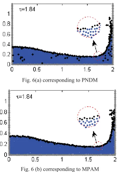
To identify the free surface particles, a new approach is developed in the paper, called MPAM. In this sub-section, some numerical results will be presented to show that it works better than the PNDM.
Fig. 6(a) corresponding to PNDM
Fig. 6 (b) corresponding to MPAM
Fig. 6 Comparisons of particle configurations obtained by using different free surface identification techniques (black
color indicates free surface particles)
For this purpose, we will again consider the case in the above sub-section withD =0.1. The case is simulated by using the MPAM and the PNDM, respectively. Particle configurations obtained by using the two different techniques at an instant are shown in Fig. 6. Fig. 6 (a) is the results corresponding to the PNDM while Fig. 6 (b) is these corresponding to the MPAM. This figure clearly demonstrates that many inner particles are wrongly identified as free surface particles by the PNDM but are correctly judged as inner particles by the MPAM. It also shows that the PNDM assigns some free surface particles to inner particles in the enlarged area but the MPAM does not make such a mistake.
5.3 Validation and convergence study
So far, we have not shown any comparison of our numerical results with experimental data nor given any discussion about the convergence property of the proposed method when it is used to simulate breaking waves. These will be addressed in this sub-section. In mesh-based methods, the convergence property is related to the element (or cell size) size in meshes or grids and time step ('W ). In meshless methods, like MLPG_R method, there is no mesh at all. Therefore, element (or cell) size is not relevant. A similar quantity is the distance between particles. Unfortunately, the distance continuously varies when modeling water waves. To bypass the problem, the initial distance of two adjoining particles is chosen as a representative distance. As the initial distribution of particles is uniform in the paper, the representative distance is equal to the difference in the x- or z- coordinates of two adjoining particles, which is denoted by 'xin the following discussion.
The two parameters ('xand 'W ) can be considered directly for studying the convergence property. They can also be replaced by other two parameters, such as 'x 'W and 'x. We prefer the second way because the later is related to the well-known Courant number that has a form of 'W ct'x
( 't ct'x gd in dimensional form) with
c
t being a constant, as used by a number of researchers studying waves, for instance, Grilli, Guyenne and Dias (2001) and Yan and Ma (2009).The case considered here is about the propagation of solitary waves over a beach with a slope of 1:15. The solitary wave is generated by a piston-type wavemaker according to the theory given by Goring (1978), in which the motion of the wavemaker is defined in dimensionless form by
>
FW O@
W k
k h
xp( ) tanh ( )tanh , where h is the wave height,
4 / 3h
k , F(W) k
>
cWxp(W)O@
and the dimensionless celerity c (1h). The experimental data for this case are [image:9.595.68.274.257.557.2]Fig. 7 Illustration of model set-up for the solitary wave
10.5 11 11.5 12 12.5 13 13.5
-0.2 0 0.2 0.4 0.6 0.8 1
x
K
Experiment
'x/'W=2.5
'x/'W=5
'x/'W=7
'x/'W=9
W=9.29
10.5 11 11.5 12 12.5 13 13.5
-0.2 0 0.2 0.4 0.6 0.8 1
x
K
Experiment
'x/'W=2.5
'x/'W=5
'x/'W=7
'x/'W=9
W=9.87
10.5 11 11.5 12 12.5 13 13.5
-0.2 0 0.2 0.4 0.6 0.8 1
x
K
Experiment
'x/'W=2.5
'x/'W=5
'x/'W=7
'x/'W=9
W=10.35
11 11.5 12 12.5 13 13.5
-0.2 0 0.2 0.4 0.6 0.8
x
K
Experiment
'x/'W=2.5
'x/'W=5
'x/'W=7
'x/'W=9
W=10.73
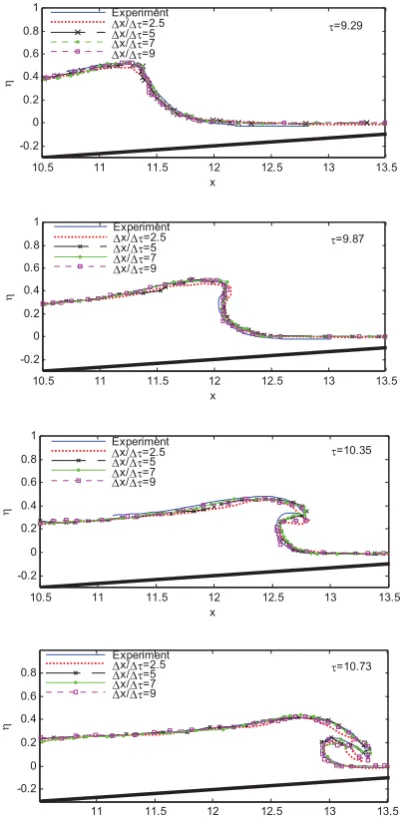
Fig. 8 Comparison between experimental wave profiles (Li and Raichlen, 1998) and numerical results for different
values of 'x'W
Firstly, we look at how the ratio, 'x 'W , affects numerical results. For this purpose, the representative distance, 'x, is taken as 0.05, corresponding to Nz =20, which yields the total
particle number of 5893. The values of 'x 'W are chosen as 2.5, 5.0, 7.0 and 9.0, respectively. The solitary wave is generated by the wavemaker, which propagates to the beach and then evolves to overturning and breaking. The part of the process is illustrated in Fig. 8 by snapshots at several instants, which are obtained by using different values for 'x 'W . For the purpose of comparison and validation, the experimental data from Li and Raichlen (1998) are also plotted in Fig. 8. It can be seen that at about W 9.29, the wave crest becomes very steep; then at W 9.87, a plunging jet starts to be formed; and after this, the jet is moving forward and nearly impacts on the other part of the water surface in its front at time W 10.73. There is no experimental data after this instant. For validation purpose, we only present the results until this instant here.
It can also be seen that the numerical wave profiles generally agree well with the experimental ones except for those corresponding to'x 'W 2.5. In addition, the numerical
results for 'x 'W 5 and 'x 'W 7are a bit closer to the experimental data than that for 'x 'W 9. This seems to imply that for a certain value of'x, the time step should not be too large or too small. It is easy to understand why the time step should not go beyond the upper limit but the reason why it is also subjected to the lower limit from the point of view of accuracy needs to be further studied. Nevertheless, one should not choose too small time step in practice in order to save computational time if possible and so the lower limit may not be of a huge concern.
It is worth noting that Yan and Ma (2009) and Grilli, Guyenne and Dias (2001) both have concluded that one may takect 0.4in'W ct'x to simulate 2D overturning solitary
waves using fully nonlinear potential theory for the finite element and boundary element simulations, respectively, which corresponds to 'x 'W 2.5 . This investigation seems to suggest that the time step for the MLPG_R method based on the NS equation should be smaller (about half in this case) than that in the methods for potential theory to achieve similar accuracy. The information is useful because it helps researchers to guess the suitable time step a prior from experience in using potential theory.
Secondly, we look at how the results vary by changing the value of 'xwith'x 'W 5. For this purpose, three different values for 'x are chosen. They are 0.05, 0.04 and 0.033, respectively. The corresponding numerical results are plotted in Fig. 9 together with the experimental data of Li and Raichlen (1998). This figure indicates that all these results up to W 10.73 have an acceptable agreement with the experimental one. It also indicates that 'x 0.05 is sufficient for the results in Fig. 8.
Wavemaker
beach d=1
10
h
[image:10.595.69.270.241.653.2]10.5 11 11.5 12 12.5 13 13.5 -0.2
0 0.2 0.4 0.6 0.8 1
x
K
Experiment
'x=0.05
'x=0.04
'x=0.033
W=9.29
'x/'W=5
10.5 11 11.5 12 12.5 13 13.5
-0.2 0 0.2 0.4 0.6 0.8 1
x
K
Experiment
'x=0.05
'x=0.04
'x=0.033
W=9.87
'x/'W=5
10.5 11 11.5 12 12.5 13 13.5
-0.2 0 0.2 0.4 0.6 0.8 1
x
K
Experiment
'x=0.05
'x=0.04
'x=0.033
W=10.35
'x/'W=5
10.5 11 11.5 12 12.5 13 13.5
-0.2 0 0.2 0.4 0.6 0.8 1
x
K
Experiment
'x=0.05
'x=0.04
'x=0.033
W=10.73
[image:11.595.69.270.98.526.2]'x/'W=5
Fig. 9 Comparison between experimental wave profiles [Li and Raichlen (1998)] and numerical results obtained by using
different 'x values when 'x 'W 5
Nevertheless, it does not mean all the values are equally good beyond that instant. In order to show this, some snapshots for later instants are plotted in Fig 10, which illustrates the wave profiles after the jet impacts the front part of the water surface, called as post-breaking stage. As can be observed, another jet is formed and a cavity behind the jet appears after the impact. It is also observed that the profiles for 'x 0.04 (Nz=25) and 'x 0.033 (Nz=30) are quite similar but there is a significant discrepancy between the one for
05 . 0
'x and others. Although the experiential data is not available for the profiles in these instants, one may deduce that 'x 0.05may not be sufficiently small to model the
post-breaking waves. In other words, more particles are required to model the waves in this stage.
12.5 13 13.5 14 14.5 15 15.5
0 0.2 0.4 0.6 0.8
x
K
'x=0.05
'x=0.04
'x=0.033
W=11.1
'x/'W=5
12.5 13 13.5 14 14.5 15 15.5
0 0.2 0.4 0.6 0.8
x
K
'x=0.05
'x=0.04
'x=0.033
W=11.4
'x/'W=5
12.5 13 13.5 14 14.5 15 15.5
0 0.2 0.4 0.6 0.8
x
K
'x=0.05
'x=0.04
'x=0.033
W=11.7
[image:11.595.314.521.138.401.2]'x/'W=5
Fig. 10 Wave profiles in the post-breaking stage obtained by using different values of 'x at when 'x 'W 5
Fig. 11 Sketch of the problem about a solitary wave propagating to and over the step
5.4 Further validation
To further validate the method, another case is considered, which has been experimentally studied by Yasuda, Mutsuda and Mizutani (1997). The sketch and the coordinate system are illustrated in Fig. 11, in which there are three wave gauges P1, P2 and P3 located at x= 6.45, 8.11 and 9.74, respectively, to measure the wave elevations at the different positions. The solitary wave height is h=0.423. The particle number (Nz) along the z-axis is 33 in the part before the step and is 5 over the step, respectively. The total particle number
S
wavemaker
0
6.45 6.45
P1 P2 P3
1
0.848
h
x
z
[image:11.595.305.531.471.573.2]used in this case is 14806. The representative distance is chosen as 'x 0.03. Taking 'x 'W 5, the time step is 0.006.
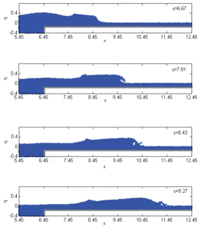
The solitary wave is generated by the piston-type wavemaker amounted at the left side of tank in the same way above. At earlier stage, the solitary wave propagates towards the step without deformation. When it reaches the step, a part of the wave is reflected and other part of the wave is transmitted to the area over the step. The front of the transmitted wave becomes steep and a jet is formed near its crest. Then the wave overturning and breaking occur. To illustrate the process, four snapshots of solitary wave profiles over the step at different time steps are shown in Fig. 12. One can observe that a plunging jet is formed and almost hits the free surface at 81W 7. . After the jet impacts the free surface, an cavity appears and the second plunging jet is formed at W 8.43. This process is largely similar to that for the solitary wave propagating over a sloped beach.
[image:12.595.311.521.98.238.2]The time histories of the wave elevations recorded at the three wave gauges are shown in Fig. 13, together with the corresponding data from Yasuda, Mutsuda and Mizutani (1997). As can be seen from the figure, the wave form recorded at Gauge P1 is still similar to a full solitary wave form, but the maximum wave height is higher than the height atx=0. At Gauges P2 and P3, the wave elevations grows quickly but the wave height is relatively smaller compared with the height at x=0. This indicates that the wave has become very steep or broken before the points. As can also be seen, the numerical results are in very good agreement with the experimental data [Yasuda, Mutsuda and Mizutani 1997] at all the gauges. That again shows that the MLPG_R method works well in the cases with violent breaking waves.
Fig. 12 Snapshots of solitary wave evolution over the step at different time steps
0 2 4 6 8 10
-0.1 0 0.1 0.2 0.3 0.4 0.5 0.6
W
K
[image:12.595.70.272.474.703.2]Exp at P1 Exp at P2 Exp at P3 Num at P1 Num at P2 Num at P3
Fig. 13 Comparisons of wave elevations between the numerical results (line) and experimental data (mark) (Yasuda et al, 1997) at three different gauges (P1, P2 and P3)
6 Conclusions
In this paper, the MLPG_R method is extended to simulate 2D violent breaking waves. Compared with our previous work, the method is improved mainly in two aspects: (1) introducing an extra term in the governing equation for pressure and (2) suggesting a new approach (MPAM) for identifying the free surface particles. Numerical tests on different configurations under different wave conditions show that the improved method can yield satisfactory results for breaking waves, which agree reasonably well with experimental results.
Acknowledgement
This work is sponsored by The Leverhulme Trust, UK, to which the author is most grateful.
References
Arefmanesh, A.; Najafi, M.; Abdi, H. (2008): Meshless Local Petrov-Galerkin Method with Unity Test Function for Non-Isothermal Fluid Flow, Computer Modeling in Engineering & Sciences (CMES), Vol. 25, No. 1, pp. 9-22.
Atluri, S.N.; Shen, S. (2002): The Meshless Local Petrove-Galerkin (MLPG) Method: A Simple & Less-costly Alternative to the Finite Element and Boundary Element Methods, Computer Modeling in Engineering & Sciences (CMES), Vol. 3 (1), pp. 11-52.
Atluri, S.N.; Zhu, T. (1998): A New Meshless Local Petrov-Galerkin (MLPG) Approach in Computational Mechanics,
Computational Mechanics, Vol. 22, pp. 117-127.
Atluri, S.N.; Zhu, T. (2000): New Concepts in Meshless Methods, International J. Numerical Methods in Engineering, Vol. 47 (1-3), pp. 537-556.
Atluri, S.N. (2005): Methods of Computer Modeling in Engineering and the Sciences. Vol. 1, Tech Science Press. Atluri, S.N.; Liu, H.T.;Han, Z. D. (2006): Meshless Local
for Solid Mechanics, Computer Modeling in Engineering & Sciences (CMES), Vol. 15, No.1, pp. 1-16.
Batra, R. C.; Ching, H.-K. (2002): Analysis of Elastodynamic Deformations near a Crack/Notch Tip by the Meshless Local Petrov-Galerkin (MLPG) Method, Computer Modeling in Engineering & Sciences (CMES), Vol. 3 (6), pp. 717-730.
Belytschko, T.; Lu, Y. Y.; Gu, L. (1994): Element-Free Galerkin methods, Int. J. Numr. Meth. Eng., Vol. 37, pp. 229-256.
Bonmarin, P (1989): Geometric Properties of Deep-Water Breaking Waves,” J. Fluid Mech. 209, 405.
Cai, Y.C.; Zhu, H.H.(2008): A Local Meshless Shepard and Least Square Interpolation Method Based on Local Weak Form, Computer Modeling in Engineering & Sciences (CMES), Vol. 34, No. 2, pp. 179-204.
Chen, S. S.; Liu, Y. H.; Cen, Z. Z. (2008): A Combined Approach of the MLPG Method and Nonlinear Programming for Lower-Bound Limit Analysis, Computer Modeling in Engineering & Sciences (CMES), Vol. 28, No. 1, pp. 39-56.
Ching, H. K.; Chen, J. K. (2006): Thermomechanical Analysis of Functionally Graded Composites under Laser Heating by the MLPG Method, Computer Modeling in Engineering & Sciences (CMES), Vol. 13, No. 3, pp. 199-218.
Dang, T. D.; and Sankar, B. V. (2008): Meshless Local Petrov-Galerkin Micromechanical Analysis of Periodic Composites Including Shear Loadings, Computer Modeling in Engineering & Sciences (CMES), Vol. 26, No. 3, pp. 169-188
Devrard, D; Marcer, R.; Grilli; ST, Fraunie, P; Rey, V, (2005): Experimental Validation of a Coupled BEM-Navier-Stokes Model for Solitary Wave Shoaliing and Breaking”. Proc. 5th Intl. on Ocean Wave Measurement and Analysis, pp 166-176.
Gao, L.; Liu, K.; Liu, Y. (2006): Applications of MLPG Method in Dynamic Fracture Problems, Computer Modeling in Engineering & Sciences (CMES), Vol. 12, No. 3, pp. 181-196.
Goring, DG (1978): Tsunamis the Propagation of Long Waves onto A Shelf, Report No. KH-R-38, W.M.Kech Laboratory of Hydraulics and Water Resources, California Institute of Technology, Pasadena, CA. pp 337.
Gotoh, H.; Sakai, T (2006): Key Issues in the Particle Method for Computation of Wave Breaking,” Coastal Engineering, 53 (2-3), pp 171-179.
Grilli, ST; Guyenne, P; Dias, F (2001): A fully non-linear model for three-dimensional overturning waves over an arbitrary bottom, Int. J. Numer. Meth. Fluid., Vol 35, pp 829–867.
Greaves, D. (2009): Application of the Finite Volume Method to the Simulation of Nonlinear Water Waves”, Ch 10 in ADVANCES IN NUMERICAL SIMULATION OF NONLINEAR WATER WAVES (ISBN: 978-981-283-649-6 or 978-981-283-649-7), edited by Q.W. Ma, scheduled to be published in Spring 2009 by The world Scientific Publishing Co.
Han, Z. D.; Atluri, S. N. (2004a): Meshless Local Petrov-Galerkin (MLPG) Approach for 3-Dimensional Elasto-dynamics, Computers, Materials & Continua, Vol. 1 (2), pp. 129-140.
Han, Z. D.; Atluri, S. N. (2004b): Meshless Local Petrov-Galerkin (MLPG) Approaches for Solving 3D Problems in Elasto-statics, Computer Modeling in Engineering & Sciences (CMES), Vol. 6 (2), pp. 169-188.
Han, Z. D.; Liu, H. T; Rajendran, A. M.; Atluri, S. N. (2006): The Applications of Meshless Local Petrov-Galerkin (MLPG) Approaches in High-Speed Impact, Penetration and Perforation Problems, Computer Modeling in Engineering & Sciences (CMES), Vol. 14, No. 2, pp. 119-128.
Idelsohn, S.R. ; Storti, M.A. ; Onate, E (2001): Lagrangian Formulation to Solve Free Surface Incompressible Inviscid Fluid Flows, Comput. Methods Appl. Mech. Engrg. Vol 191, pp 583-593.
Issa, R; Violeau, D; Lee, ES; Flament, H (2009): Modelling Nonlinear Water Waves with RANS and LES SPH Models, Ch 14 in ADVANCES IN NUMERICAL SIMULATION OF NONLINEAR WATER WAVES (ISBN: 978-981-283-649-6 or 978-981-283-649-7), edited by QW Ma, scheduled to be published in 2009 by The world Scientific Publishing Co.
Jarak, T.; Soric, J.; Hoster, J. (2007): Analysis of Shell Deformation Responses by the Meshless Local Petrov-Galerkin (MLPG) Approach, Computer Modeling in Engineering & Sciences (CMES), Vol. 18, No. 3, pp. 235-246.
Khayyer, A; Gotoh, H (2008): Modified Moving Particle Semi-implicit Methods for the Prediction of 2D Wave Impact Pressure, Coastal Engineering, doi: 10.1016/j.coastaleng. 2008.10.004.
Khayyer, A; Gotoh, H; Shao, SD (2008): Corrected Incompressible SPH Method for Accurate Water-Surface Tracking in Breaking Waves, Coastal Engineering, Vol 55, pp 236-250.
Klessfsman, KMT; Fekken, G; Veldman, AEP; Iwanowski, B; Buchner, B (2005): A Volume-of-Fluid Based Simulation Method for Wave Impact Problems, Journal of Computational Physics, Vol 206, pp 363-393.
Koshizuka, S; Oka, Y (1996): Moving-Particle Semi-Implicit Method for Fragmentation of Incompressible Fluid,
Nuclear Science and engineering, Vol 123, pp 421-434. Lee, BH; Park, JC (2007): Numerical Simulation of Impact
Loads Using a Particle Method, MPS, Proceeding of the Seventeenth International Offshore and Polar Engineering Conference, Lisbon, Portugal, July 1-6, pp 2029-2036. Li, Y; Raichlen, F (1998): Discussion- Breaking Criterion
and Characteristics for Solitary Waves on Slope, J. Waterw., Port. Coastal, Ocean Eng., Vol 124, pp 329-335. Li, Y; Raichlen, F (2003): Energy Balance Model for
Breaking Solitary Wave Runnup, J. Waterw. Port. Coastal, Ocean Eng., Vol 129, pp 47-59.
Method, Computer Modeling in Engineering & Sciences (CMES), Vol. 26, No. 1, pp. 61-74.
Li, S; Atluri, S.N., (2008b): The MLPG mixed collocation method for material orientation and topology optimization of anisotropic solids and structures, Computer Modeling in Engineering & Sciences (CMES), Vol. 30 (1): 37-56. Lin, P. Z; Liu, Philip L.-F (1998): A numerical study of
breaking waves in the surf zone, J. Fluid Mech, vol. 359, pp. 239-264.
Lin, H.; Atluri, S.N. (2000): Meshless Local Petrov-Galerkin (MLPG) method for convection-diffusion problems,
Computer Modeling in Engineering & Sciences (CMES), Vol. 1 (2), pp. 45–60.
Lin, H.; Atluri, S.N. (2001): The Meshless Local Petrov-Galerkin (MLPG) method for solving incompressible Navier-Stokes equations, Computer Modeling in Engineering & Sciences (CMES), Vol. 2 (2), pp. 117-142. Lo, E.Y.M.; Shao, S.D. (2002): Simulation of near-shore
solitary wave mechanics by an incompressible SPH method”, Applied Ocean Research, Vol 24, pp275-286.
Ma, Q.W. (2005a): Meshless Local Petrov-Galerin Method for Two-dimensional Nonlinear Water Wave Problems,
Journal of Computational Physics, Vol 205, Issue 2, pp 611-625.
Ma, Q.W. (2005b): MLPG Method Based on Rankine Source Solution for Simulating Nonlinear Water Waves, Computer Modeling in Engineering & Sciences (CMES), Vol. 9, No 2, pp 193-209.
Ma, Q.W.; Yan, S (2006): Quasi ALE Finite Element Method for Nonlinear Water Waves, Journal of Computational Physics, 212, pp 52-72.
Ma, Q.W. (2007): Numerical Generation of Freak Waves Using MLPG_R and QALE-FEM Methods, Computer Modeling in Engineering & Sciences (CMES), Vol.18, No.3, pp.223-234.
Ma, Q.W. (2008): A New Meshless Interpolation Scheme for MLPG_R Method, Computer Modeling in Engineering & Sciences (CMES), Vol 23, No 2, pp 75-89.
Ma, Q.W. (2009): MLPG_R Method and Its Applications to Various Nonlinear Water Waves, Ch 15 in ADVANCES IN NUMERICAL SIMULATION OF NONLINEAR WATER WAVES (ISBN: 283-649-6 or 978-981-283-649-7), edited by QW Ma, scheduled to be published in 2009 by The world Scientific Publishing Co.
Mohammadi, M. H. (2008): Stabilized Meshless Local Petrov-Galerkin (MLPG) Method for Incompressible Viscous Fluid Flows, Computer Modeling in Engineering & Sciences (CMES), Vol. 29, No. 2, pp. 75-94.
Miyata, H (1986):Finite-difference simulation of breaking waves,Journal of Computational Physics, Vol. 65, issue 1, pp. 179-214.
Monaghan, JJ (1994): Simulation Free Surface Flows with SPH, Journal of Computational Physics, Vol. 110, pp 399-406.
Nayroles, B.; Touzot, G.; Villon P. (1992): Generalizing the Finite Element Method, Diffuse Approximation and Diffuse Elements, Computational Mechanics, Vol. 10, pp. 307-318.
Onate, E; Idelsohn, S; Zienkiewicz, OC; Taylor, RL; Sacco, C (1996): A stabilized Finite Point Method for Analysis of
Fluid Mechanics Problems, Comput. Methods Appl. Mech.
Engrg.139: pp 315-346.
Pini, G.; Mazzia , A.; Sartoretto, F. (2008): Accurate MLPG Solution of 3D Potential Problems , Computer Modeling in Engineering & Sciences (CMES), Vol. 36, No. 1, pp. 43-64.
Rapp, RJ; Melville, WK (1990): Laboratory Measurements of Deep-Water Breaking Waves, Philos. Trans. R. Soc. London, Ser. A 3777, 311.
Sellountos , E. J.; Sequeira, A.; Polyzos, D., (2009): Elastic transient analysis with MLPG(LBIE) method and local RBFs”, Computer Modeling in Engineering & Sciences (CMES), Vol. 41, No. 3, pp. 215-242.
Shao, SD; Lo, EYM (2003): Incompressible SPH Method for Simulating Newtonian and Non-Newtonian flows with a Free Surface, Advances in Water Resource, 26 (7), pp 787-800.
Sladek, J; Sladek, V; P. H. Wen; Aliabadi, M.H. (2006): Meshless Local Petrov-Galerkin (MLPG) Method for Shear Deformable Shells Analysis, Computer Modeling in Engineering & Sciences (CMES), Vol. 13, No. 2, pp. 103-118.
Sladek, J; Sladek, V; Zhang, Ch.; Tan, C.L. (2006): Meshless Local Petrov-Galerkin Method for Linear Coupled Thermoelastic Analysis, Computer Modeling in Engineering & Sciences (CMES), Vol. 16, No. 1, pp. 57-68.
Sladek, J; Sladek, V; Zhang, Ch.; Solek, P., (2007): Application of the MLPG to Thermo-Piezoelectricity, Computer Modeling in Engineering & Sciences (CMES), Vol. 22, No. 3, pp. 217-234.
Sladek, J; Sladek, V; Solek, P.; Wen, P.H.; Atluri, S.N. (2008): Thermal Analysis of Reissner-Mindlin Shallow Shells with FGM Properties by the MLPG, Computer Modeling in Engineering & Sciences (CMES), Vol. 30, No. 2, pp. 77-98.
Sladek, J; Sladek, V; Solek, P.; Wen, P.H.; (2008): Thermal Bending of Reissner-Mindlin Plates by the MLPG, Computer Modeling in Engineering & Sciences (CMES), Vol. 28, No. 1, pp. 57-76.
Sladek, J; Sladek, V; Tan, CL; Atluri, S.N. (2008): Analysis of Transient Heat Conduction in 3D Anisotropic Functionally Graded Solids, by the MLPG Method,
Computer Modeling in Engineering & Sciences (CMES), Vol. 32 (3): 161-174.
Yasuda, T.; Mutsuda, H.; Mizutani, N. (1997): Kinematics of overturning solitary waves and their relations to breaker types, Coastal Engng. 29, 317-346.
Yan, S, and Ma, Q.W., (2009): QALE-FEM for modelling 3D overturning waves, accepted for publication by
International Journal for Numerical Methods in Fluids.
Zhang, S; Morita, K; Kenji, F; Shirakawa, N (2006): An Improved MPS Method for Numerical Simulations of Convective Heat Transfer Problems, International Journal for Numerical Methods in Fluids, pp 51: 31-47.
Vavourakis, V.; Sellountos, E. J.; Polyzos, D. (2006): A comparison study on different MLPG(LBIE) formulations, Computer Modeling in Engineering & Sciences (CMES), Vol. 13, No. 3, pp. 171-184.
Wang, K.; Zhou, Shenjie; Nie, Zhifeng; Kong, Shengli, (2008): Natural neighbour Petrov-Galerkin Method for
Shape Design/Sensitivity Analysis, Computer Modeling in Engineering & Sciences (CMES), Vol. 26, No. 2, pp. 107-122.
Wu, N.J. ; Tsay, T.K. ; Young. D.L. (2006): Meshless numerical simulation for fully nonlinear water waves,
![Fig. 9 Comparison between experimental wave profiles [Li and Raichlen (1998)] and numerical results obtained by using](https://thumb-us.123doks.com/thumbv2/123dok_us/1622182.115327/11.595.314.521.138.401/comparison-experimental-profiles-raichlen-numerical-results-obtained-using.webp)