Computational methods for contact stress problems with normal and tangential loading

Theses

Thesis/Dissertation Collections

1991

Computational methods for contact stress

problems with normal and tangential loading

Christopher R. McGoldrick

Follow this and additional works at:

http://scholarworks.rit.edu/theses

This Thesis is brought to you for free and open access by the Thesis/Dissertation Collections at RIT Scholar Works. It has been accepted for inclusion

in Theses by an authorized administrator of RIT Scholar Works. For more information, please contact

[email protected].

Recommended Citation

Computational Methods for Contact Stress

Problems with Normal and Tangential Loading

Christopher R. McGoldrick

Master of Science Thesis

1991

Rochester Institute Of Technology

College of Engineering

Department of Mechanical Engineering

Approvals:

J0seph Torok - Thesis Advisor

.Richard Budynas

Richard Hetnarski

Mark Kempski

I

Christopher R. McGoldrick

hereby grant permission

to

Wallace Memorial Library

of

Rochester Institute of Technology

to reproduce my thesis

in

whole or part.

Thesis

Abstract:

Computational

Methods for Contact

Stress

Problems

with

Normal

and

Tangential Loading.

Christopher

R.

McGoldrick

Master

of

Science

Mechanical

Engineering

Rochester

Institute

Of

Technology

Rochester,

New York

January,

1991

This

investigation

contains an

historical

overview of contact stresses

including

various classifications of

the

problem and

their

associated solutions.

The

solution

for

the

normal

loading

elliptical contact problem

is

reviewed,

as

formulated

using

classic methods of

linear elasticity

theory.

An

efficient computational method

is

developed

to

evaluate

the

elliptic

integrals

that

arise.

The

limitations

of

this

solution are

investigated

in detail

and

it is

shown

how

the

method could

be

extended

to the

sliding

elliptical

1.

Introduction

1

1.1. What

are contact stresses?

1

1.2.

Why

they

are

important

1

1.3. Nature

of

the

Applied

Loading

1

1.4.

The

Continuum

Model

3

1.5. The

Elastic Foundation Model

5

1.6.

Coordinate

System

For

Non-conforming

Single Point Contact

5

1.7. Milestones

in Contact

Stress

Development

7

1.8.

The Proposed Computational Method

8

2. Classification

of

Contact Stress Problems

10

2.1.

Relevant Factors

10

2.2.

The Rigid Punch

and

Other Stiff

Geometries

10

2.3.

Elastic

Half-Spaces

11

2.4.

Rolling

Contact

12

2.5. Plastic

Deformation

13

2.6.

Conforming

Contact

14

2.7.

Numerical Methods

15

2.8.

Hertzian

Contact

16

2.8.1.

Elliptical

Contact: "The

General

Case"

16

2.8.2.

Limitations

or

Bounds

of

the

Hertz

Theory

17

2.8.3.

Extension

of

Hertzian Contact

17

3. The

Geometry

of

Contact

19

3.1.

Local

Surface

Geometry

19

3.2. Combinations

of

Bodies

22

3.3.

Magnitude

Checks

23

4.

Elasticity

Methods

27

4.1.

Equilibrium

27

4.2. Strain

at a

Point

28

4.3.

Compatability

Equations for

Linear Strain

29

4.4.

Hooke'sLaw

30

4.5. Stress

Functions

30

11

5.

Axisymmetric

Solids

of

Revolution

33

5.1. Stresses

and

Deformations

in

a

Solid

of

Revolution

33

5.2. Concentrated

Normal

Force

36

5.3. Distributed

Normal Loads

38

5.4. Spherical

Contact

41

5.5. Cylindrical

Contact

-

Another Two-Dimensional

Case

48

6.

Elliptical Contact

50

6.1.

Surface

Geometry

for

Elliptical

Contact

51

6.2. Development

of

Equations

for

Elliptical

Contact

55

6.3.

Elliptical

Solution Overview

57

6.4.

An Elliptic Integral Primer

59

6.4.1. Complete

Elliptic Integrals

60

6.4.2.

Incomplete Elliptic Integrals

62

6.5.

Explicit Numerical Procedures

for

Normally

Loaded Elliptical

Contact

63

6.6.

Application

of

the

10-Step

Method

to

Determine Maximum

Stress

Values

69

6.7. Contact Stresses

101 (Benchmark

Testing)

73

6.8.

The

Real Contact Problem

76

6.8.1. Surface

Displacements

77

6.8.2. Surface Stresses

77

7.

Practical

Applications

79

7.1.

Gaussian Profiles

and

the

Rusty

Nail

79

7.1.1.

On

Surfaces

and

Their

Statistical

Descriptions

79

7. 1

.2.

Measurement Techniques

81

7.1.3.

Mathematical

Surface

Models

82

7.1.4. True Contact Area

84

7.2.

The Real

Structure

of

the

Surface Layers

of

Metallic

Bodies

84

7.3.

Friction Between Real

Surfaces

85

7.3.1. The

Classic

Laws

of

Friction

85

7.3.2. Theories

of

Friction

86

7.3.3.

Rough

Surfaces

and

Friction

87

7.3.4.

Design Tips

for

Friction Calculations

88

7.4.

Lubrication

and

Pitting

Failure

89

7.5. Impact

on a

Worn

Surface

90

7.6.

Rolling

Contact

and

Shakedown

91

7.7.

Allowable

Stresses

92

7.8.

Heat

Treating

and

Contact Stresses

92

7.8.1.

Nitriding

93

7.9.

Gears

95

7.10.

Camrollers

96

7.11.

Wheel

and

Rail

97

8.

Summary

98

8.1.

On

the

useof

the

Continuum Model

to

Describe

Real Materials

98

8.2.

On

the

Elliptical Solution Implemented

in

this

Investigation

98

8.3.

Tangential

Loading

for

Elliptical

Contact

99

8.4.

Direction

for

Future Work

99

9. A Personal Note

101

Introduction

1

1. Introduction

1.1. What

are contact

stresses?

Contact

stresses are caused

by

the

pressure of one solid on another over

limited

areas of contact.

They

are

merely

the

localized

stress

distributions

at and near

the

surface of

the

body.

Contrast

this

to the

axial stress on a cylindrical

tensile test

specimen

in

which

the

engineering

stress represents

the

bulk behavior.

Even

there,

the

stress

distribution

normal

to

the

cross-section

is

not uniform when

necking

starts

to

occur.

The

stresses on

the

surface ofa

body

outside

the

contact

area(s),

where

there

are no applied

tractions,

must

be

zero

for

equilibrium.

This

is

a

boundary

condition

for

some solutions.

Stresses

inside

the

contact area are

merely

the

internal

reaction ofone

body

accommodating

the

intrusion

ofanother.

The

point where

the

force is

applied moves a small amount

in

response

to the

load.

This

occurs

because both

the

supporting

and

contacting

materials are not

rigid

or

fixed

in space,

but

have

finite

stiffnesses associated with

them.

As

a

result, the

bodies

are not

necessarily fixed

in

their

geometry

over

time.

Contact

stresses are

localized

reactions,

so

that

Saint Venant's Principle

applies

to their

analyses.

The

study

of contact stresses

is

often avoided

because

the

mathematics

is difficult

and

does

not

lead

to

solutions

in

terms

of

formulas

which can

conveniently be

used

by

designers.

1.2.

Why

they

are

important.

The

premature

failure

of

many

machine elements can

be

attributed

to

excessively

high

contact stresses.

In

some

cases,

the

maximum stress

due

to

contact

between

mem

bers

is

regarded as a

limiting

criterion of

design. Inaccurate

calculation or neglect of

their

effects

is

a common

design

flaw.

Some

classic contact stress problems

involve

ball

bearings,

cylindrical

rollers,

gear

teeth,

and wheels on a

track.

The

loading

in

these

cases

is

often cyclic.

Repeated

loading

is

related

to

microscopic

failure

phenomena such as

cracking, pitting,

and subsurface

fracture.

1.3. Nature

of

the

Applied

Loading

The

method used

to

determine

contact stresses

depends

on

the

initial

contact geome

try

and

the

applied

load.

Limited

cases of closed-form solutions are

available,

some of which will

be

reviewed

in

this

investigation.

Two-dimensional

solutions can often

be

Special

consideration

is

given

to

computation of stress

inside

the

area of contact.

The

normal and

tangential

stress

distributions

are

typically

calculated

independently

and

then

superimposed.

The

normal

force

N

is

traditionally

assumed

to

be

directly

propor

tional

to the

friction

or

tangential

force

F,

with

the

constant of

proportionality

being

the

coefficientof

friction

1,

that

is

F

= _/*N.

(1.1a)

The

symbols

P

for

normal

force

and

Q

for

tangential

force

are

commonly

used

in

the

contact mechanics

literature

and will

be

used

here.

Equation 1.1a

which

follows

the

notation

found in

introductory

physics and statics

textbooks, is

an oversimplification of

the

relation

between

normal and

tangential

loading.

In

reality

the

normal and

tangential

loads,

and

the

coefficient of

friction,

are

distributed functions

over

the

contact area so

the

relationship

between

them

is

more

adequately

represented

by

Q(x,y)

=

M(x,y)

P(x,y).

d.lb)

If

adhesive

forces

at

the

interface

are

neglected,

the

presence of

any

tangential

load

must

be

associated with a normal

load. For analysis,

it is

assumed

that there

is

no

interaction

or

coupling between

the

normal and

tangential

force distributions

other

than

that

given

by

Equation

1.1b.

Including

tangential

loading

in

the

analysis

is necessary

for

a realistic model of

the

contact

between

machine

elements, but

it significantly

in

creases

the

complexity

of

the

solutions such

that

a computer

is

required.

The

contact

geometry

also affects

the

form

ofthe pressure

distribution between

the

bodies

as

in

the

cases of

line,

spherical,

and elliptical contact which

have

uniform,

spherical,

and ellipsoidal

distributions,

respectively.

Contact

stresses,

like

all

stresses,

have

a

three-dimensional

character

(See Figure 1.1). Spherical

and cylindrical contact are often approximated as

two-dimensional

problems

to

simplify

the

analysis and yield

insight into

the

overall

behavior.

Long

rollers

in

contact

(plane strain)

or

thin

disks

(plane

stress),

will

in

reality

experience end-effects

that

will create

three-dimensional

stress

distributions.

The

presence of

friction,

which

breaks

any symmetry

of

the

problem

that

was

due

to the

geometry,

also necessitates a

three-dimensional treatment.

'. figure 1.1 Differential

stress element

for

three

Introduction

1.4. The

Continuum

Model

You

are

here.

Figure 1.2

Family

of material models. Branchesof mechanics are not a_{clearly defined hierarchical} treebuta more nebulous cluster of relationships andinterconnectionsthat overlap,liketheneurons thatcreatedthem.

The

material model

for

the

contact stress problems

discussed

throughout

this

investigation is based

on

linear

elasticity.

It

borders

however

on

plasticity

theory

in

determining

the

onset and

definitions

of

yield,

which

is

of critical

importance

to

designers.

The

three-dimensional

nature of contact stresses

therefore

requires an

understanding

of stress as a

tensor

quantity

and

its

associated principal values

(See

Figure 1.3).

The

principal stresses are used

in

conjunction with material properties

to

determine

if

a given

geometry

can withstand

the

applied

loading

without

yielding,

or

if

yielding

does

occur,

its

extent.

Every

material

has

different

deformation

response characteristics

to

applied

loads,

as

r _For1-3plane

Assume a\ >_^>a^>0

"X

(c)

<

Viewsof element ondifferentprincipalaxes

-+-F

Rough

(o) Rigid

-PerfectlyPlaatlc

*|

Wfflr_-I

VWJM//W////AW/W>.

Rough

() Elastic-_PerfectlyPlatte

|

WWV 1

illustrated

by

a stress-strain

diagram.

This

data is

typically

obtained

from

the

tensile

test

of a circular rod.

One

of

the

tasks

of

the

stress analyst

is

to

relate

the

stateofstress

for

this

simple configuration

to

a more complex

three-dimensional

situation.

The

effect of

attaining

a certain stress

level depends

on

the

model of

the

material.

Figure

1.4

illustrates

a

few

of

the

commonly

used

idealizations

of stress-strain curves used

for

calculating

plastic

behavior.

The

final

stress state

is

path-dependent

if

the stress

levels

go

beyond

the

material's elastic

limit.

This

means

that the

sequence or order

in

which

the

loads

are applied

that

cause plastic

deformation

determines

the

final

stress state.

The

framework

for

this

investigation is

the

realm of continuum mechanics and

theory

of

elasticity

(see

Figure

1.2).

The

determination

of contact stresses

has

its

roots

in

linear

elasticity

theory

which

is based

on

the

continuum model of material

behavior.

The

continuum model assumes

the

material

to

be

continuous,

homogeneous,

and

usually

isotropic. These

assumptions allow

field

quantities such as stress and

displacement

to

be

expressed as piecewise continuous

functions.

The

earliest models of contact problems were analyzed as concentrated

loads

applied

to

an

infinite

elastic medium.

These

solutions provided

insight

into

the

overall

behavior

of concentrated

loads,

but

contained singularities.

Singularities

and

the

infinite

stresses and

deformations

associated with

them

are not possible

in

real materials.

WS/S////AW//AV//AW//MW, Rough

() RigidLinearWorkHardening

i

WAV

E,

|

M |MVWI

v/)m>MJ>mm/ww/w/m

Rough

(rf) ElasticLinear Work_Hardening

Figure

1.4 Continuummodels of materialbehavior

Most

materials exhibit a

strong

temperature

dependence,

usually softening

with

increasing

temperature.

The

rate at which

the

load

is

applied

(strain rate)

can also

have

an effect on

the

stress-strain curve.

A

category

of materials exists called

visco-elastic,

that

exhibit

time-dependent

responses

to

stress.

The

stress-strain curve

is

a useful

idealization,

but in

reality

each material possesses a stress response

function

that

is

a multi-dimensional surface

described

by

the

variables

strain,

strain

rate,

temperature,

and

time,

to

name a

few. The

computational method

developed

in

this

investigation

Introduction

1.5. The

Elastic

Foundation

Model

One

ofthe

early

models

developed

to

analyze contact phenomena

treated

the

material

like

a

bed

of springs as shown

in Figure 1.5.

This

was

done

to

avoid

having

to

solve an

integral

equation

for

pressure.

The bed

of springs

is

presumed

to

be

penetrated

by

a

rigid

indenter. The

contact pressure at

any

point

depends only

on

the

compression of

the

spring

at

that

point.

Point

contacts or

indentation

by

bodies

with

very

small radii are not modeled

adequately because

there

is

no support

from

adjacent

springs.

The

model gives useful

first

approximations

to

problems

in

which

the

bodies

cannot

be

locally

represented

by

principal curvatures.

This

model

has

proved useful

in

analyzing rolling

contact with

tangential

loading

and problems

involving

visco-elastic

bodies [1]. Elastic foundation

type

models are sometimes used

in

concrete slab

design

in

order

to

calculate

the

required

thickness to

withstand

building

column

loads.

Figure 1.5 The

elastic

foundation

model.

1.6.

Coordinate System For

Non-conforming

Single

Point

Contact

Before

we can

discuss any

particular method of

solution,

it is

useful

to

define

a coordinate system which can serve as a

framework

to

survey

the

entire

field

of contact mechanics.

The

definitions

and

figures

in

this

section are

from

Johnson

[1].

When

brought into

contact,

non-conforming

surfaces will

initially

touch

at a point

or

line if

one of

the

bodies

is

cylindrical.

The

contact area

is

generally

assumed

to

be

small compared

to

the

dimensions

of

the

bodies

themselves.

The

origin of

the

coordinate system

is

taken to

be

the

point of contact.

The Z

axis

is

taken to

coincide

with

the

common normal

to the two

surfaces.

The X-Y

plane

is

called

the tangent

plane.

The

undeformed shapes of

the two

surfaces are specified

by

the

functions:

zl

=

f^x.y)

_and

Zj

=

f2(x,y).

The

separation

between

them

before

loading

is

given

by:

h

=

Figure 1.6

Generalcoordinatesystem

for

contact problems.

In applications,

contact

may involve

complex motions such as

those that

occur

between

gears and

self-aligning

bearings. The

motion of a

body

at

any instant in

time

is

described

by

its

linear

and angular

velocity

vector with respect

to the

contact point.

The

following

terms

are used

frequently

in

the

literature,

so

they

are

defined

here

with reference

to the

general coordinate system shown

in

Figure 1.6.

Sliding:

relative

linear velocity between

the two

surfaces.

Rolling:

relativeangular

velocity

between

the two

bodies

about an axis

lying

parallel

to the tangent

plane.

Spin:

relative angular

velocity

about

the

common normal.

M,<^

^

r>-M*JX

S > <jA

^V

\&

y

^^^^s**^

^x

25ffi2i

Z

Introduction

Figure 1.7

shows

that the

net tangential

force

can

be

resolved

into

two

components

Qx

and

Qy. The force

transmitted

at

the

point of contact

has

the

effect of

compressing

the

deformable

solids so

they

effectively

make contact over an area of

finite

size.

This

makes

it

possible

to transmit

a resultant moment

in

addition

to

a

force

which could not occur

if

contactwas

truly

at a single point.

The

components

Mx

and

My

are

defined

as

rolling

moments and are part of what causes

"rolling

resistance".

The

component

Mz

accounts

for friction inside

the

contact area and

is

called

the

spin moment.

1.7. Milestones in Contact Stress Development

The

following

section

highlights

some of

the

major

stepping

stones

to the

work

in

this

investigation.

Significant

developments

are

identified

in

the

mathematical

formulation

and treatmentof

the

problem,

but

it is

by

no means an exhaustive

summary

of all

the

work

in

the

field

of contact mechanics.

Most

developments in

the

theory

did

not appear until

the

beginning

of

this

century,

when needed

by

the

railway, gear,

and

bearing

industries.

Theoretical

developments

seemed

to

have

stopped

in

the

mid

nineteen-sixties, due

to

lack

of computational power

to

carry

out

the

integral

solutions.

Research

in

numerical methods continues

however.

(1881)

Heinrich Hertz

[2]

invented

the

classical

theory

of contact stresses

in

his

paper

"On

the

Contact of

Elastic

Solids".

At

age

24,

Hertz

was

working

as a research assistant

to

Helmholtz

at

the

University

of

Berlin.

He

was

studying

the

optical

interferences

in

glass

lenses

and

the

effect of

clamping forces

on

the

fringe

patterns.

He

made an

analogy

between

contact pressure andelectrostaticpotential

theory.

His

solution gave

only

the

principal stresses

in

the

contact area

but has

been

extended over

the

years

to

cover a wide

variety

of physical

cases,

at

least

as a

first

approximation and

benchmark.

(1930)

H.R.

Thomas

and

V.A. Hoersh

[3]

transformed the

Hertzian

solution

for

stresses on

the

axis of

symmetry

into

standard elliptic

integrals

and

discovered

that

the

shearing

stress

distribution

along

the

axis

has

a maximum at some

distance beneath

the

contact area.

This

showed

that

a method of

failure

which

initiated

below

the

surface,

such as

pitting,

could

be

explained

by

the

existenceof

these

maximum shear stresses.

(1939)

G.

Lundberg [4]

considered

the

effect of a

tangential

load between

arbitrary

surfaces.

He

introduced

three

potential

functions corresponding

to the

components of

loading

along

the

axes of a

Cartesian

coordinate

(1949)

R.D.

Mindlin

[5]

showed

that

the

solution of

the tangential

and normal

pressure

distributions

can

be

decoupled

without

introducing

significant error.

The degree

of approximation

is

of

the

same order as

neglecting

the

small shear

tractions

in

the

Hertzian

problem with

dissimilar

materials.

He

developed

the

theory

of

slip between

the

contact surfaces.

An

undesirable characteristic of

his

solution

is

that

the

traction

approaches

infinity

at

the

edges,

which

is

not

physically

possible.

Presumably,

the tangential

component of

traction

cannot exceed

the

productof

the

coefficient of

friction

1

and

the

normal

load.

For

the

case of circular contact under

spin,

it is

shown

how slip

penetrates

from

the

outer radius

a,

to

an

inner

radius

a',

and

that

in

the

included

annulus,

the

traction

remains at

the

greatest possible value of

lp.

With

increasing

torque,

slip is eventually initiated

over

the

entire contact area.

Where

there

is

no

slip, displacements

on

the two

bodies

must match.

(1951)

Cheng Kang

Liu

[6]

and also

in

an oft-cited reference with

J.O.

Smith

[7]

investigated

both

normal and tangential

loads

that

were assumed

to

have

an ellipsoidal

(Hertzian)

distribution

over

the

contact area.

The

magnitude of the

intensity

of

the

tangential

load is

assumed

to

be

linearly

proportional

to

that

of

the

normal

load

when

sliding

motion

is

impending.

The

stresses

in

the

body

are presented

in

closed

form

for

both

the

plane stress and plane strain problems.

A

numerical value of

V3

wasassumed

for

thecoefficient of

friction.

They

discovered

that

when

the

tangential

loads

are applied at

the

contact

area, the

maximum

shearing

stress

may be

at

the

surface

instead

of

beneath it. This is

a most

important

result

in

that

it

explains real

failure

phenomenon such assurface crack propagation.

1.8. The Proposed Computational Method

In

his

thesis

[6],

Liu

formulates

the

solution

to

the

three-dimensional problem with

normal and

tangential

loads in

terms

of

integrals.

He

states

the

need

for

a

feasible

way

of

evaluating

the

integrals. The

computational power now exists

to

perform

these

calculations.

The

main portion of

this

investigation

resulted

in

computer programs

to

evaluate

these

integrals

within

the

framework

of

the

contact stress

problem,

making

this

a

feasible

course of action.

The

method

developed

in

this

investigation is

based

on

the

notation and equations

from

Seely

and

Smith

[8],

which were originated

by

Liu.

Seely

was

Liu's

thesis

Introduction

9

evaluated

by

numerical

methods,

which makes

the

calculation of contact stresses an

inherently

numerical problem.

The

program

treats

stress as a

tensor

quantity

to

reinforce

its

three-dimensional

nature,

which

is

so often overlooked.

The

method of

determining

contact stresses

by

evaluation of

the

elliptic

integrals,

and

its

implementation

as a computer

program,

forms

the

central work of

this

investigation.

The

computer programs used

to

implement

these

calculations could

be

developed

into

a

tool to

be

used

in

product

development,

failure

analysis,

and as a

pedagogical

tool

in

the

classroom as well.

The

calculation of

contact stresses

is

an

2.

Classification

of

Contact

Stress Problems

2.1. Relevant Factors

There

are

many factors

to

consider when

modeling

a contact problem.

Problems

do

not

always

fit into

neat categories and there will

be

cross-over

between

classifications.

Some

of

the

relevant

factors

are as

follows:

o

Geometry:

Is

the

problem

two

orthree-dimensional?

If

two-dimensional,

is

it

plane stress or plane strain?

Is

there

single, multiple,

or

conforming

(close-fit,

nearly contacting)

contact?

What is

the condition of each sur

face? Are

they

rough orsmooth?

o

Loading:

Are

there

normal or tangential

loads,

or

both? Is

the

loading

cyclic?

What

is its

magnitude?

Is it

a point or

distributed load?

o

Relative

motion:

Does

rolling, sliding,

or

torsional

motion occur

between

the

bodies,

or

is

there

impact?

o

Deformation: Are large

strains

present,

as

is

likely

with elastomers?

Is

there

plastic

deformation?

o

Thermal

effects:

Is it

a problem concerned

primarily

with

heat

transfer

through

the

interface

or

does

a

thermal

stress

field

needto

be

superimposed

onthe

mechanically

imposed

stresses?

o

Materials: Are

the

materials

isotropic,

anisotropic,

or

possibly

visco-elas-tic?

o

Relative

stiffness

between

the

bodies:

Should it be

treated

as arigidpunch problem?

All

of

the

above

factors

are

important

in

determining

which solution methods are applica

ble

to a specific problem.

For

the

purposes of this

investigation,

the

following

classifications

have

been found

to

be

useful.

2.2.

The Rigid Punch

and

Other Stiff

Geometries

Problems in

which one

body

has

a

significantly

higher

elastic modulus

than the

other

can

be

treatedas a

"rigid

punch"

Classification

11

shapes

have been

studied such as

blunt

ends, tapered wedges, cones,

and spheres

(See

Barber

[9],

Galin

[10],

Gladwell

[11],

and

Nadai

[12]).

Tangential

loading

is

not

usually

associated with

this type

of problem.

I

/

-Qy-r-rr/

-it

Figure 2.1 Rigidpunchindentation.

Another group

ofproblems

in

whichone

body

is

consideredrigidcompared to theother

is

the

rolling

of metals.

These involve

thermal

effects,

as

in

the case of

hot rolling

and

plasticity

with

work-hardening

for

cold

rolling

operations.

2.3.

Elastic Half-Spaces

An

elastic

half-space is defined

as a semi-infinite elastic solid

bounded

by

a planesur

face. It is

one

half

of a

Cartesian

space,

usually identified

withtheplusorminus z regions.

However,

it is

often convenient to use polar coordinates with the origin centered at the point of contact.

Deformations

are

taken

to

be

linearly

proportional to the

forces. The

differential

equations of equilibrium and

the

compatibility

relations

from elasticity

are

assumed to apply.

The

surface outside

the

contact region

is free

of

stresses,

within the

region

it is loaded

by

the

prescribednormal and

tangential

pressure

distributions. At large

distances

from

the

loading

zone,

thestresses musttend tozero.

The

elastic

half-space

idealization

amounts

to

ignoring

the effects of one of the

contacting

bodies

with the purpose of

simplifying

the

boundary

conditions.

Solutions

typically

give

infinite

stresses at the point of

contact,

which cannot

physically

exist,

but

area

property

of

the

solution.

The

overall stress patterns

have been

verified

by

photoelas-tic

and

finite

element methods.

The

idealization

gives someusefulresults and

in fact

forms

the

basis

for

more general methods.

Tangential

and normal

loads

for

line

and point

contact

have been investigated

for

two

and

three-dimensional

cases.

Figure

2.2 illustrates

2.4.

Rolling

Contact

Rolling

contact problems are

treated

as separate phenomena.

Rolling

(contact)

is de

fined

as relative angular motion

between

two

bodies

about an axis parallel

to

their com

mon

tangent

plane.

The frame

ofreferenceas

defined

in

section

1.6 is

consideredto move

with

the

point of contact.

If

the velocities

V1

and

V2

are

unequal,

the

rolling

motion

is

accompanied

by

sliding.

If

theangular velocities

ozl

and

o^

are

unequal,

it is

accompanied

by

spin.

The

terms

free

rolling

and tractive

rolling

areused

to

describe

motions

in

which

the

net

tangential

force

Q

is

zeroand

non-zero,

respectively

[1].

In

steady

rolling,

the strain

field does

not change with

time.

The

resultant tangential

traction

must not exceed

its

limiting

value which

is

theproduct ofthe coefficient of

fric

tion

and the resultant normal

force.

Freely

rolling

bodies

having

dissimilar

elastic properties will

develop

different

tangential strains.

A

special case

involves

two elastic

bodies

which are

geometrically

identical

and

have

the same elastic

properties.

That

is,

they

are

completely

symmetrical about

their

interface. When

rolling

under

the action of a

purely

normal

force,

notangential tractionor

slip

can

occur,

so the contact stresses

and

deformations

can

be

approxi mated

by

the static

Hertz

distribution

[1].

b a

" dl

Pis ^r ~AW

' *.'

-\f '_{'_.} B

\

_{C(x. 0)}

s

\

r

AOr,z)

'' z

Figure 2.2 Distributednormal andtangentialloads.

Sliding

is

not as straight

forward

since some portions of

the

contact area

may

slip

or possess

relative

motion,

while the remainder

does

not and sticks

together.

A difference between

the

tangential

strains

in

the

two

bodies

in

the

sticking

area

leads

to a small apparent

slip,

called creep.

Sticking

and

micro-slip

zones

form

in

the contact area

in

relative proportions and

locations

that are

determined

by

the

interaction between

friction

forces

and elastic

deformations.

To determine

the

stresses

in

the

body,

an

Eulerian

point ofview

is

taken

in

which

the

material

is

considered

to

move past

the

point of contact.

The

equilibrium of surface elements

is formulated in

terms

of

their

velocity

vectorswhich

have

components

from

the

strain rates andthe

velocity

of

the

bodies

as awhole.

This

technique

allows

the

differences

in

surface strains

to

be

accounted

for,

which give risetoslip.

The

boundary

conditions

for

the

strain-derived

differential

equations of equilibrium

are,

for

steady rolling

contact:

Classification

13

2)

Tangential

traction

is limited

by

the

coefficient of

friction.

3)

Direction

of

tangential

tractionmust opposeslip.

These

conditions aremodified

(meaning

increased

complexity)

to

account

for

tractive

rolling,

and

differing

amounts of

slip from

complete

slip

to

none.

They

become

quite complex

for

three-dimensional

bodies

with

traction,

spin,

and

transient

behavior occurring

during

start-up.

For

visco-elastic

rolling, the

problems of compression and

rolling-sliding

must

be

distinguished,

even when

friction is

absent,

due

to the

time-dependence of the stress-strain

law.

Rolling

contact will not

be

covered

further

in

this

investigation. It

was mentioned

for

completeness andto

help

illustrate

thecomplexities associated with contact problems.

2.5. Plastic

Deformation

Problems

involving

plastic

deformation

require special

treatment

because

the

final

stress state

is

path-dependent.

This

state

depends

on

the

material model

used,

i.e. perfectly

plastic, elasto-plastic, etc.,

and onthework

hardening

modelused

(if

any).

See Mendelson

[15]

for

theories

on

kinematic

and

isotropic

hardening. Follansbee

and

Sinclair

[16]

have

studiedthe

indentation

of a

ball

well

into

the

fully

plasticstate.

Such

workcould

be

usedto

develop

an accurate model of

hardness

testing.

The

initial

phases of a standard

hardness

test

can

be

treated

as a classic contact stress problem

up

to

thepoint ofplastic

deformation.

An

experimentaltest stand shown

in Figure

23

could

be built

to measure the

force

and

deflection

of an

indenter

as

it

waspressed

into

a material.

It

would

be

set

up for

automatic

data

acquisition

enabling

the test

data

to

be

correlated

to

the theoretical model.

Such

a system could also

be

used to test various

indenter

shapes and sizes as well as

for

the

analysis of rigid punch phenomena

by

using

sharp-edged

indenters. A holographic

stress analyzer could record

the

fringe

patterns of surface

deflection

in

real

time

and

they

could

then

be

correlated with

theoretical

predictions.

PC

BASED

DATA

AQUISITIDN

LINEAR

TRANSDUCER

MDTDRIZED

DR

HYDRAULIC

PRESS

LDAD

CELL

CHANGABLE

INDENTDR

TIPS

?F

VARIDUS

SHAPE, SIZE,

AND

HARDNESS.

TEST

SPECIMEN

RIGID

BASE

2.6.

Conforming

Contact

Conforming

contact arises

from

thegeometric condition

in

which the two

bodies

are separated

by

a small

distance

over appreciable portions of

their

surfaces.

Here,

the

geometry

before

and after

loading

is known

ahead of

time.

For light

loads,

thecontact area will

be

small

in

relation

to

the radii ofthe

bodies.

As

the

load becomes

larger,

the contact

area grows

rapidly

to

become

asignificant

fraction

of

the total

surface

area,

which violates

the

Hertzian

assumptions.

Such

a condition can

be

more

suitably

treated

by

methods appropriateto

conforming

contact.

This is

an example of

how

the magnitude ofthe

load

can

determine

the

applicable solution method.

Examples

of

conforming

contact are a

cylinder

in

atight

fitting

hole,

initially

contacting

along

a

line,

and a sphere

in

a spherical

cavity

where

the

magnitude of the radii of the

bodies

are

very

close.

For

these simple geometries at

light

loads,

thestresses and

deformations

predicted

by

Hertzian

theory

are accurate.

As

the

load is

increased,

the stresses

in

the

conforming

case will

be lower

because

the

supporting

area

increases

at a

faster

rate than predicted

by

Hertzian

theory.

The deformations

will

be

smaller

because

oftheadditional support offered

by

thesecond

body.

Numerical

methods are needed

to

solve

conforming

contact problems.

Paul

and

Hashemi

[17]

have

studied contact pressures on

closely conforming

elastic

bodies

and

have developed

a numerical method

for frictionless

surfaces.

Their

work

includes

a

technique

for

automatically generating

meshes that

overlay

the

load-dependent

contact

patches.

The

following

is

anoutline ofthemethod:

A

Cartesian

coordinate system

is

set

up,

with the

initial

contact point as

thecommon origin.

The

initial

separation

between

points onthe two

bodies

is known. The

effect at each point

resulting

from

the

deformation

of

neighboring

points,

is

weighted

by

an

influence function

and summed up.

Using

indenters

of prescribed

finite

curvature,

a

fictitious interpenetration

is

generated.

The bodies

are

discretized into

subregions and a system of

linear

equations

is

set

up

that

determines

the

deformations

from

the

penetration at

neighboring

points

by

superposition.

Stress

evaluation points aretaken

to

be

atthecentroids ofthecells.

If

boundary

conditions are not

satisfied,

a newpenetration curve or contact

boundary

is

generated.

This is

done

iteratively

until

satisfactory

convergence occurs.

Finite

element programs areused

to

generate

the

interpenetration

curves.

The

restrictions ofthemethod

include

the assumptions that thecontactregion

is

assumed

to

be

symmetricalabout one axis

in

the tangent plane, the

initial

contact

is

at a single

point,

Classification

15

Figure 2.4 BlanketandContact Area froma numerical method

by

SinghandPaul.

2.7.

Numerical

Methods

Numerical

methods

typically

involve

discretization

of the

domain. Figure 2.4 is

an example

of a numerical method

by

Singh

and

Paul

[18]

in

which

the

pressure

function

p(x,y)

is

replaced

by

a piecewise constant

pressure

field.

Note

the

large

gradients near the edges of

the

grid.

They

report that the

simply-discretized

method

is numerically

unstable

in

the general case.

Instability

arises

because

the

solution vector to the set of

linear

algebraic equations

is

very

sensitive

to

small perturbations

in

the elements ofthecoefficient matrix.

Large

oscillations

in

the solution vector correspond

to

small variations

in

the elements of the coefficient matrix.

Since

perturbations are unavoidable

in

the process of

creating

the grid,

convergence to the

solutionvector

tends to

be very

erratic.

This

discrete

method

is incapable

of

predicting

the

proper stress

distribution in

non-symmetric problems.

For

non-symmetric

cases,

stabilizing

techniques were

introduced

which

they

call the

"Redundant Point Field

Method"

and the

"Functional Regularization Method". Both

of

these

significantly

increased

theamount of

computation required.

As

a refinement of

the

procedure techniques need

to

be

found

to

eliminate

the

singularities

occurring

near

the

edges ofthegrid.

On

the

other

hand,

the

large

scale solution

is very

good and

friction

effects are accounted

for.

Other

numerical solutions

include finite

element methods.

A

commercially

available

code

that

handles

three-dimensional contact

has been recently developed [19]. The

drawbacks

to

the

finite

element

method,

based

on

the

amount of

memory

required

for

available commercial programs

to

run and

the

size of

their

data

files,

arethat

it:

o

is

computationally

extensive.

o

does

not

readily

lead

to

parameterization

studies,

although

parametrically

generated

FEA

models could

be

generated.

o calculates stresses and

deformations

throughout

theentire

field

when,

during

initial design

phases,

only

critical

design

parameters are sought such as

orders ofmagnitude or maximum values of stress at a particular

location

etc.

2.8. Hertzian Contact

The

pioneering

work of

Hertz

[2]

includes

theclassic contact stress solution and was

the

first

theoretical

work

done

in

thisarea.

Elastic

contact stress problems areclassifiedas

Hertzian if

they

satisfy

the

following (five)

conditions:

1)

The

bodies

are

homogeneous, isotropic,

obey

Hooke's

Law,

and experience small strains and

rotations,

i.e.

smallstrain elasticity.

2)

The

contacting

surfaces are

frictionless.

3)

The dimensions

ofthe

deformed

contact patch remainsmall comparedto the

principalradii oftheundeformed surfaces.

4)

The deformations

arerelated to thestresses

in

thecontactzonesas predicted

by

the

linear

theory

of

elasticity

for half

spaces.

5)

The

contacting

surfaces are continuous and

may

be

represented

by

second-degree

polynomials

(quadratic surfaces)

prior

to

deformation.

The majority

of work on contact stress

is based

on the assumption that the contact region

is

theellipse predicted

by

Hertzian

analysis.

The

equations

for

circular contact areas will

be developed later in

this

investigation

to

familiarize

readers with theproblem.

These

solutions can

be

expressed as simple

formulas

sothegeneral concepts and

behavior

can

be

illustrated before

proceeding

to

the more general case of elliptical contact areas which

is

the

central

topic

of

this

investigation.

2.8.1. Elliptical

Contact:

"The

General

Case"

The

mostgeneralcase

has

no

symmetry

aboutthesurface normalto the tangentplane.

Tangential

loading

also

destroys

the

symmetry

of the problem.

Major

results

for

the

general case of

Hertzian

contact are as

follows:

o

The

contact area

is bounded

by

an ellipse which can

be

calculated

from

the

geometric configuration:

the

principal radii ofthe

bodies

and the relative angular orientation oftheprincipal planes.

o

The dimensions

of

the ellipse,

a and

b,

increase

directly

as the cube root of

the

load P.

Classification

17

2xab

o

Regions

of

the

solidswhichareremote

from

thecontactzone approacheach

other

by

an amount whichvariesasP( \

o

The

principal stresses are all compressive.

The

maximum

shearing

stress occurs

below

thesurface.

Note

the non-linear

dependence

on the

load

of the contact area and

deflection. The

same

formulas

hold for both

solids

using

the appropriatevalue of

Poisson's

ratio,

v.

See

section

5.2

on

Spherical Geometries for

general numerical conclusions.

Thomas

and

Hoersh

[3],

and

Lundberg

[4]

show that variations of

Poisson's

ratio

in

the usual

engineering

range

do

not

have

a

strong influence

on the

important features

ofthe stress pattern.

It

may

still affectthemagnitudeofthe

results,

so the propervaluesshould

be

used

for design

problems.

Special

cases ofthegeneral

Hertzian

problem arethose of spherical

and cylindrical contact.

The

equations

in

these

simple cases

do

not

involve

elliptic

integrals,

however

thepresenceof

friction

greatly

increases

theircomplexity.

2.8.2. Limitations

or

Bounds

of

the

Hertz

Theory

The Hertz

theory

has been

confirmed

by

numerous experiments.

Haines

and

Ollerton

[20]

report

that the

Hertz

theory

accurately

predicts

the

shearstresses

for

elliptical contact where

the

semi-major axis of the ellipse of contact

is

as

large

as one-half the smallest radius of curvature of either of

the

contacting

solids.

The

geometric predictions of the

theory

cannot

be

expected

to

be

accuratewhenthe

deviations

from

the

original

hypothesis

arethis

large. Beyond

theelastic

limit,

someoftherelationscontinue to

be

approximately

valid,

but

the

deviation

increases

withthe

degree

of

departure

from linear

elasticity.

2.83.

Extension

of

Hertzian

Contact

Several

departures

from

the

original

hypotheses have been

developed,

including

higher-order

polynomialstomodelthe

initial

geometry.

The

polynomial corrections are on

thesameorder of magnitude as

the

assumptions of

the

linear

elasticity

theory

itself

so this

is

not a productive

avenue,

except

for

cases of

conforming

contact.

Dissimilar

materials

have

also

been

studiedand some parameters

developed

to

account

for

therelative stiffness

between

the two

bodies. Contact

of rough surfaces

has been

modeled

by

assuming

that the

bodies

are covered with an

array

of

hemispherical

protrusions called asperities.

This is

an

attempt

to

determine

the

true contact area and relies

heavily

on statistical methods.

For

Attempts

have

been

madeto

incorporate friction

in

the

Hertzian

results.

The

so-called

Smith-Liu Equations

[7]

solve the two-dimensional cylindrical problem with tangential

loading.

The

solution

does

notcontainelliptic

integrals,

but

the

computations arestill

very

tedious.

Analytical

solutions

have

been developed

for

sliding

spherical contact

by

Goodman

and

Hamilton

[21]

which are more

like

explicitly-specified procedures rather

thansimple

formulas.

In

this

investigation

a numerical method

is defined

as one

in

which the

domain is

decomposed

into discrete

regions or

substructures,

versus a computational

one which evaluates thestress

field

at

any

continuous coordinate

based

onthe continuum

Geometry

of

Contact

19

3.

The

Geometry

of

Contact

3.1. Local

Surface

Geometry

Two

bodies in

contact are presumed

to

touch

initially

at a single point.

The

curvatureof each

body

is

modeled

by

two

radii,

the

principal and

secondary,

which are associated with

the

maximum and minimum surface curvatures of

the

body

at

the

contact point.

The

planes

containing

the

maximum and minimum curvatures are orthogonal.

When

two

bodies

are

considered,

the

principal planes of each will not

necessarily

coincide so

the

angle

between

the

planes of principal curvature must

be

considered.

The

complete

geometry

can

therefore

by

specified

by

four

radii and

the

angular orientation

between

the

principal axes.

The

angle of orientation a

is

meaningless

if

either one of

the

bodies

is

axisymmetrical, in

which case

it is

assigned a

value of 0

for

calculation purposes.

Negative

radii

indicate

that the

center of curvature

for

that

principal plane

lies away from

the

body,

i.e. it is

a concave surface.

The

classification of a given

geometry

and

its

subsequent mathematical

treatment

depends

on

the

sign and relative magnitude of

the

four

radii.

'. Figure 3.1

Body

with positive principal and

secondary

radii of curvature.

The

following

is

a rationale

for

the

use of

two

radii

to

describe

the

local

surface

geometry.

In

modeling

a

continuum,

it

can

be

assumed

that

the

surface

has

a

continuous

curvature,

that

is,

there

areno

discontinuities in

the

region near

the

contact point.

Mathematically,

this

means

that the

slopes must

be

continuous at all points on

the

surface.

The

simplest continuous

functions

that

satisfy

this

requirement are second order

polynomials,

since

by

taking

their

second

derivative

with respect

to

displacement,

Figure

3.2

Local curvature

does

not_necessarily

representtheoverall shape of a

body.

locally

describe

a surface

leads

to

expressions

having

similar

form

but

containing

more

terms.

This

approach

is

used

in

problems

involving

conforming

contact

[22].

There

is

a

branch

of mathematics

called

differential

geometry

in

which

physical quantities such as

length

take

on

infimtesimal

values.

Differential

geometry

is

the

study

of geometric

figures using

the

methods of calculus.

A

well-known

theorem

states

that

any

surface can

be

locally

characterized

by

two

principal radii.

This

abstraction

is

acceptable

for

contact stress

analysis,

since we are

only

concerned with

local

effects near

the

point of application of

the

load.

A

surface

in

E3

(three-dimensional

Euclidean

space)

is

uniquely determined

by

certain

local

invariant

quantities called

the

first

and second

fundamental

forms.

These

quantities

depend only

on

the

surface and not the particular representation

(coordinate

system).

Another

differential

geometry

theorem

states

that:

For

every

point

P

on a

surface,

there

exists a coordinate patch

containing

P

such

that the

directions

of

the

u

and v parameter curves are principal

directions.

See Lipschutz

[23]

for

more on

this.

Gaussian curvature,

another

invariant,

is

the

product of

the

principal and

secondary

curvatures of

the

body. While

it is

not used

in

the

determination

of stresses and

displacements,

it

could

be

a useful characterization of

the

surface

for

possible use as a variable

in

a

dimensional

analysis

study

of

ball

bearing

failure

rates.

The

theorems

and

derivations

of

differential

geometry

do

not

play

a role

in

the

actual

determination

of

contact stresses.

The

point of

mentioning

them

is

to

show

that

a surface

described

locally by

two

curvatures

is

not

just

a physical convenience

introduced

to

solve

the

problem,

but

also

has

a sound mathematical

basis.

Figure

3.2

illustrates

that

the

bodies

themselves

can

be

quite

arbitrary

and

irregular.

It

is

easier

to

visualize

the

contact

if

you project or extend

the

local

radii

which characterize

the

surface

to

create a complete object.

Various

combinations of

numeric sign and magnitude of

the

principal and

secondary

radii can

be

thought

of as

representing different bodies

such as spheres and cylinders.

Eight

types

of

these

bodies

can

be

distinguished

as

defined in

Table

3.1.

These

are not

necessarily

the

overall

shape of

the

bodies in

contact,

although

they

could

be.

If

the

radii

that

characterize

the

surfaceat

any

given pointare

extended,

they

would

form

whole

bodies in

these

shapes.

The

curvature

may be completely different

at another point on

the

surface of

the

body,

but it

can not

be

drastically

different if

it is in

the

vicinity

of

the

contact point.

The

Geometry

of Contact

21

Body

Type

Principal

Radius

R

Secondary

Radius

R'

Visualize

I

+

+

Football

II

+

-Hyperboloid

III

-

-Elliptical Crater

IV

+

equals

R

Sphere

V

-equals

R

Spherical Seat

VI

+

00

Cylinder

VII

- 00

Cylindrical

Trough

VIII

00 00

Plane

Table

3.1

Body

Types aredefined

by

thesignand relative magnitude oftheprincipal radii.

The

need

for

this

classification arose

in

the

computer

implementation

of

the

analysis

of contact stresses.

Certain

cases or combinations of

these

"bodies" require special

mathematical

treatment

to

avoid

division

by

zero and other computer-related

peculiarities.

The

need

to treat

certain geometries as special cases

is

not mentioned

anywhere

in

the

literature.

Many

authors

develop

integral

equations

to

solve

for

contact

stresses

but

mention

nothing

about

how

to

implement

them,

which

introduces doubt

as

to

whetheror not

they

were ever used

to

actually

calculate anything.

Figure

3.3

Body

Type

I

Figure 3.4

Body

Type II

Figure 3.7 The

TorusorDonut

Figure

3.8

Body

Type VHI

The

most general

body,

one with unequal positive principal

curvatures,

is

termed

"Body

Type

I"

and

is

illustrated in Figure

3.3.

The

inverse

of

this

is

both

curvatures

being

negative as seen

in

Figure

3.5.

Body

Type

II

shown

in

Figure

3.4

is

characterized

by

one positive and one negative radius.

Figure

3.6

shows

Body

Type

IV,

the

convex sphere.

The

simplest

body

type

is

a sphere with a radius of one unit.

Body

Type

V,

the

concave

sphere,

is

realized when

both

radii are equal and negative.

This

type

of surface could

be

produced

by

a

ball

end mill.

The

torus

shown

in Figure

3.7

is

not one of

the

body

types

itself,

but

the three

points

A, B,

and

C

can each

be

represented

by

a

different

one.

The

torus

was

included

to

show

that

the

local

curvature

should not

be

confused with

the

geometry

as a whole.

Body

Type

VIII,

shown

in

Figure

3.8,

is

"The

Plane" and

is

characterized

by

both

radii

being

infinite.

When

one

of

the

bodies

is

a plane or spherical

type,

the

angle a

becomes irrelevant due

to

symmetry.

3.2. Combinations

of

Bodies

Although

there

areno restrictions on

the

values of

the

radii on an

individual

body,

other

than

being

non-zero,

there

are restrictions when two

bodies

are considered.

Certain

combinations of radii and angular orientation produce geometries

that

are

physically

impossible

for

a single-pointcontact problem.

The

following

figures

provide a graphic

illustration

of some of

the

combinations of

body

types.

When

two

cylinders are placed

in

contact,

they

may

produce elliptical or

line

contact

depending

on

the

relative angular orientation.

Figure

3.9

shows

the

caseof

line

contact

between

cylinders

in

which case a

is 0.

A

special case occurs when

two

cylinders of equal

diameter

are crossed at

90,

producing

a circular contact area.

An

experimental apparatus such as

this

can

be

used

to

test

coefficients of

friction

and

wear-rates

between

various materials

because

the

area can

be easily

predicted and

the

sliding

Geometry

of Contact

23

this

case

is

not

the

same as

the

spherical case of equal area and normal

force,

because

the

secondary

radii are

infinite.

Consider

an

arbitrary

point on

the

surfaceof

the

solid near

the

contactpoint.

A

sphere

contacting

another sphere or a plane will

both

produce circular contact areas.

Now

move some

distance

outside

the

contact

area,

keeping

a constant z elevation.

In

the

first

case of

two

spheres,

this

location is

outside either of

the

bodies

while,

in

the

second case

it

remains on

the

surface of

the

plane.

The

stress

distributions

cannot

be identical because

there

is

not a one-to-one

mapping

of

the

geometries.

The

maximum normal pressure and stresses on

the

centerline should

be

similar

between

the two

cases

however.

Figure

3.9

Contacting

Cylinders

Line

contact can occur

if

a cylindrical or planar

body

type

is explicitly

selected or

the

eccentricity

of

the

elliptical contact area

is

so

large

that

contact

effectively becomes

a rectangle.

The

circular and

line

contactcases are simpler

than the

general case

in

that

they

it do

not

depend

on elliptic

integrals.

The

fact

that

the

elliptical solution

asymptotically

approaches

the

closed-form circular and

line

contact solutions makes

for

a good

benchmark

test

of a

"general

method".

A

feature

of

the

line

contact problem

is

that

it

cannot

be

normalized

(i.e.

mapped

onto

the

range

from

0<R<1)

because

of

the

infinite

radius

defining

a cylinder or plane.

To

normalize a

problem,

all

the

radii are

divided

by

the

magnitude ofthe

largest

radius which then

itself

becomes

unity.

In

line

contact,

the

infinite

radius would

map

all

the

other radii

to

zero.

Certain

values of

the

four

radii and

the

angular orientation can

be

specified which correspond

to

physically impossible

geometries.

For example,

a

body

with a positive radius cannot

be brought

into

single point contact with a

body

having

a negative radius of smaller magnitude than

the

positive one.

This

would

be

a

force fit.

A

mathematical solution might

be

obtained,

but it

would

be

incorrect

to

apply

the

results

to

a

design

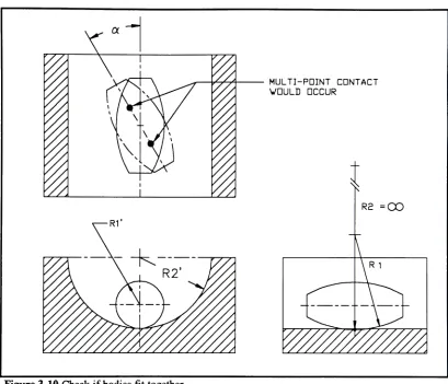
problem.

Geometries may

also

be

specified

that

are

physically

possible

but

violate

the

assumptions of

the

theory,

such as

the

case of

conforming

and multi-point contact.

3.3.

Magnitude Checks

Potentially

invalid

geometries can occur when

any

one of

the

four

radii

takes

on a negative

value,

i.e.

possesses concave curvature.

Negative

curvatures

occurring

in

the