Astronomy&Astrophysicsmanuscript no. belike °cESO 2014 May 7, 2014
R-matrix electron-impact excitation data for the Be-like
iso-electronic sequence
⋆
L. Fernández-Menchero
1, G. Del Zanna
2, and N. R. Badnell
11 Department of Physics, University of Strathclyde. Glasgow G4 0NG, United Kingdom
e-mail:[email protected]
2 Department of Applied Mathematics and Theoretical Physics, University of Cambridge, Cambridge CB3 0WA, United Kingdom
May 7, 2014
ABSTRACT
Aims.Emission lines from ions in the Be-like isoelectronic sequence can be used reliably for diagnostics of temperature and density of astrophysical and fusion plasmas over a wide range of temperatures. Surprisingly, interpolated data is all that is available for a number of astrophysically important ions.
Methods.We have carried out intermediate coupling frame transformation R-matrix calculations which include a total of 238 fine-structure levels in both the configuration interaction target and close-coupling collision expansions. These arise from the configurations
1s22{s,p}nl with n=3−7, and l=0−4 for n≤5 and l=0−2 for n=6,7.
Results.We obtain ordinary collision strengths and Maxwell-averaged effective collision strengths for the electron-impact excitation of all the ions of the Be-like sequence, from B+to Zn26+. We compare with previous R-matrix calculations and interpolated values for
some benchmark ions. We find good agreement for transitions n=2−2 with previous R-matrix calculations but some disagreements with interpolated values. We also find good agreement for the most intense transitions n=2−3 which contribute via cascade to the (n=2) diagnostic radiating levels.
Key words. Atomic data – Techniques: spectroscopic
1. Introduction
Emission lines from beryllium-like ions are used in astrophysics to study a variety of emission sources. For example, solar corona ultraviolet spectra (Vernazza & Reeves 1978; Sandlin et al. 1986) or solar flares (Neupert et al. 1967). Emission lines have been recorded by several solar missions, such as Skylab (Dere 1978). In the recent years, high-resolution XUV spectroscopic observations by Chandra and XMM-Newton satellites, have also shown that a vast number of astrophysical sources produce emis-sion lines from Be-like ions, such as Fe XXIII (Audard 2003).
Many emission lines from Be-like ions have temperature or density sensitivity, so they can be used for diagnostics of astro-physical plasmas. In particular, the intensity ratios of the reso-nance versus the intercombination transitions in the Be-like ions is an excellent temperature diagnostic. The ratio between the 2s 2p1P
1−2p2 1D2 and the intercombination transition is also a good diagnostic, considering that the lines always fall close in wavelength. Indeed, this ratio has provided one of very few di-rect measurements of electron temperatures in the solar corona from SOHO (see, e.g. Wilhelm et al. 1998). Be-like ion emission lines can be also used for diagnostics of fusion plasmas (Inoue et al. 2001; Summers et al. 1992).
Despite their importance, accurate electron impact excita-tion data for ions in this sequence are sparse. Coulomb-Born-plus-Exchange intermediate coupling calculations to n=3 were carried out by Sampson et al. (1984) for 17 ions between Ne6+ and W70+. R-matrix calculations were carried out by
Berring-⋆ These data are made available in the archives of APAP via http://www.apap-network.org and OPEN-ADAS via http://open.adas.ac.uk
ton et al. (1985) for C2+, O4+, Ne6+and Si10+ in LS -coupling followed by algebraic recoupling of the reactance matrices, only for transitions among the n=2 levels (which give rise to 10 fine-structure levels). The effective collision strengths of Berrington et al. (1985) were interpolated by Keenan et al. (1986) to provide data for N3+, F5+, Na7+, Mg8+, and Al9+. With the addition of data for Ca16+from R-matrix calculations similar to Berrington et al. (1985) by Dufton et al. (1983), Keenan (1988) provided interpolated data for P11+, S12+, Cl13+, Ar14+, and K15+. These two sets of interpolated rates have been widely used in the liter-ature, and have been included in early versions of the CHIANTI database (Dere et al. 1997).
However, the irregular contribution of resonances to eff ec-tive collision strengths along an iso-electronic sequence (Wit-thoeft et al. 2007) places an unknown uncertainty on such inter-polated data. For example, significant problems with the interpo-lated values were found by Del Zanna et al. (2008). Del Zanna et al. (2008) performed an explicit R-matrix calculation for Mg8+ and compared the intensities of the main lines with those ob-tained with the interpolated values. Significant differences (up to 50%) were found. There is therefore a need for explicit R-matrix calculations for all Be-like ions of astrophysical interest. This is the aim of the present work, which is part of a larger program of work to use the R-matrix method to calculate effective collision strengths for all ions, up to Zn, of all L-shell sequences as well as a start on the M-shell. The most recent sequence to-date is the B-like by Liang et al. (2012) and which contains references to earlier work on other sequences.
2p3d (26 terms) for Ne6+ (Ramsbottom et al. 1994a; Rams-bottom et al. 1995). Zhang & Sampson (1992) obtained fully-relativistic distorted wave collision strengths, for transitions within the n=2 complex, for all of the Be-like ions from O4+to U88+. More recent fully-relativistic work includes distorted wave data (up to 2p4d and 2s5d) for Si10+by Bhatia & Landi (2007) and R-matrix results (up to n = 5) for S12+, obtained using the Dirac R-matrix Code (DARC) by Li et al. (2013).
Because of their importance to astrophysics, extensive in-termediate coupling R-matrix calculations for Be-like iron and nickel were carried out by Chidichimo et al. (2005) and Chidichimo et al. (2003) within the Iron Project, following an early distorted wave study by Bhatia & Mason (1981). In Chidichimo et al. (2005), collision strengths and effective col-lision strength were obtained for Be-like Fe for the configura-tions n =2,3,4, including a total of 98 fine-structure levels in the basis set. A quite fine mesh was used for the electron impact energies, so the resonances were well resolved. In Del Zanna & Mason (2005), these atomic data were benchmarked against observations, pointing out temperature and density diagnostics. Overall good agreement between predicted and observed inten-sities was found. We therefore adopt this work on Fe22+ as a benchmark of the whole sequence.
We also adopt the Del Zanna et al. (2008) results for Mg8+ as a benchmark. Del Zanna et al. (2008) adopted the same target as Chidichimo et al. (2005) to calculate the scattering data for Mg8+. They also benchmarked the atomic data against SOHO spectroscopic observations of the solar corona, finding excellent agreement, thus resolving long-standing discrepancies between observed and predicted line intensities. The use of R-matrix data resulted in significantly higher electron temperatures.
Finally, we also adopt as a benchmark the R-matrix results for C2+by Berrington et al. (1985) (n=2) and Berrington et al. (1989) (n=3). In this latter case (n=3) no algebraic recoupling of the LS -coupling reactance matrices was carried out. Rather, when these data were uploaded to the CHIANTI data basis, level resolved data were obtained by splitting the LS -coupling eff ec-tive collision strengths according to statistical weights (see Dere et al. (1997)).
We note also that Mitnik et al. (2003) carried out an R-matrix with pseudostates calculation for C2+, but only in LS -coupling. They found that inclusion of pseudostates reduced effective col-lision strengths for transitions n =2−3 by typically 10% and those n =2−4 by 20−30%. Furthermore, a similar R-matrix with pseudostates calculation by Badnell et al. (2003) found re-ductions of up to a factor of two in effective collision strengths for transitions to n=4 in B+. The effect of coupling to the con-tinuum diminishes rapidly with increasing charge state though and so we would expect only modest overestimates for our N3+ data.
In the present work we include states up to n = 7 in our configuration interaction (CI) expansion, for a total of 238 fine-structure levels. This basis set includes more bound states than any other previous non-pseudostate work and so levels up to
n =4 are better represented. In addition, cascading effects fol-lowing collisional excitation up to the n=7 shell can be exam-ined with this basis set expansion. We use the same basis set and methods for the whole isoelectronic sequence, from B+to Zn26+. The present data therefore includes significantly more transitions than the previous published works for ions in the same sequence. Traditionally, astrophysics interest stops at Zn−for ex-ample, the Chianti and Cloudy modeling packages span H−Zn. This is because elemental abundance, e.g. solar, drops by over an order of magnitude at the next element
on-wards. However, we continue on up to Kr for magnetic fusion application. There-on, relativistic effects may need to be in-cluded in the wave functions themselves, e.g. via use of the Dirac R-matrix code. We leave no gaps because of the dif-ficulty of deeming a priori those elements which will never be of interest to astrophysics or, especially, magnetic fusion. Any such would be small in number and so their omission not represent any significant saving of effort.
The paper is organised as follows. In section 2 we give de-tails of our description of the atomic structure and in section 3 that of the R-matrix calculation. In section 4 we show some rep-resentative results and compare them with the previous data of other R-matrix calculations or interpolated values. In section 5 the main conclusions are discussed. Atomic units are used un-less otherwise is specified.
2. Structure
To obtain the wave functions of the isolated target we used the
program (Badnell 2011).
calcu-lates the wave functions by diagonalizing the Breit-Pauli Hamil-tonian (Eissner et al. 1974), which includes the relativistic terms, mass-velocity, spin-orbit, and Darwin, as a perturbation. The electronic potential is included in terms of the Thomas-Fermi-Dirac-Amaldi model, adjusting the scaling parametersλthrough a variational method, minimizing the equally-weighted sum of all LS term energies. We included a total of 21 atomic orbitals in the basis set: 1s, 2s, 2p, 3s, 3p, 3d, 4s, 4p, 4d, 4f, 5s, 5p, 5d, 5f, 5g, 6s, 6p, 6d, 7s, 7p, 7d. In the configuration interaction we in-cluded all the configurations 1s22s2, 1s22s 2p, 1s22p2, 1s22s nl and 1s22p nl, with nl all the orbitals previously mentioned with
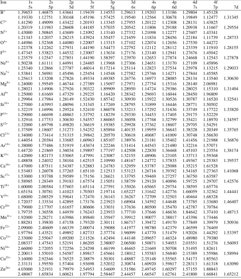
n≥3, for a total of 39 configurations. The minimized values of the scaling parameters are shown in table 3 for all the ions in the sequence. As the atomic number increases,λfor the 1s orbital increases far away from unity. This is due to the Darwin term becoming more important as the charge of the nucleus increases. This does not affect the actual atomic structure nor the values of the level energies. The values ofλfor orbitals with high angular momentum d, f and g are also much larger than the unity, which is necessary to influence the wave function for these eccentric orbits.
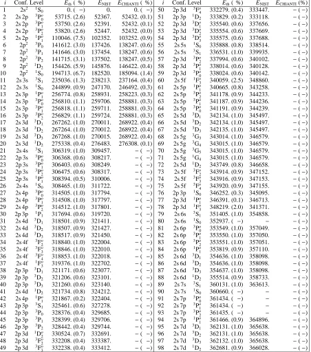
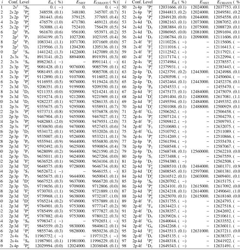
For such a configuration list we get a total of 130 LS terms, which are split into 238 intermediate coupling (IC) levels. The calculated target energies for the IC levels up to n = 4 of the sample ions C2+, Mg8+, and Fe22+ are shown in tables 4, 5, and 6, respectively. They are compared with the observed ones, taken from the National Institute of Standards and Technology (NIST1) database (Moore (1993) for carbon, Martin & Zalubas (1980) for magnesium and Sugar & Corliss (1985) for iron) and previous theoretical works collected in the CHIANTI database (Berrington et al. (1985) for carbon n = 2, Berrington et al. (1989) for carbon n=3, Del Zanna et al. (2008) for magnesium and Chidichimo et al. (2005) for iron). With a few exceptions in the lower excited singlet levels, the agreement with the observed values is within 1.5%. The deviation of the calculated energies respect the observed values is smaller in present work than in previous ones, only in the case of carbon it is larger than Berring-ton et al. (1985, 1989), this is due to their use of pseudo-orbitals. We prefer to use a spectroscopic orbitals so as to avoid having to deal with pseudo-resonances. In any case, our philosophy is to use the same approach to the structure along the entire sequence. The energy values for the rest of the levels and the other ions of
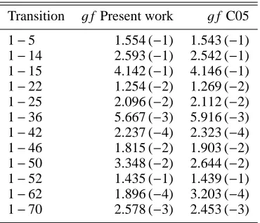
Table 1. Comparison ofgf values for some selected transitions of the
ion Fe22+. C05: Chidichimo et al. (2005). A (B) denotes A×10B.
Transition gf Present work gf C05
1−5 1.554 (−1) 1.543 (−1) 1−14 2.593 (−1) 2.542 (−1) 1−15 4.142 (−1) 4.146 (−1) 1−22 1.254 (−2) 1.269 (−2) 1−25 2.096 (−2) 2.112 (−2) 1−36 5.667 (−3) 5.916 (−3) 1−42 2.237 (−4) 2.323 (−4) 1−46 1.815 (−2) 1.903 (−2) 1−50 3.348 (−2) 2.644 (−2) 1−52 1.435 (−1) 1.439 (−1) 1−62 1.896 (−4) 3.203 (−4) 1−70 2.578 (−3) 2.453 (−3)
the sequence not shown in tables 4, 5, 6, can be found online. As with the previous sequences that we have considered, we use the calculated energies in the R-matrix calculation.
To check the quality of the calculated wave functions of the target we compare the oscillator strengths (gf values) for
se-lected transitions in Table 1 for Fe22+with data from Chidichimo et al. (2005), which can be found on line in the CHIANTI database. Very good agreement is found, with the exception of the very weak transition 1−62: 2s2 1S0−2p 4s3P1.
Fig. 1 shows a global comparison of oscillator strengthsgf
for all the transitions between the levels shown in tables 4-6, with the upper level with a configuration 2l nl′with n ≤ 4, for the benchmark ions. We plot in the x-axis the present results, and in they-axis the results of Tachiev & Fischer (1999) for carbon, Del Zanna et al. (2008) for magnesium, and Chidichimo et al. (2005) for iron. We note that the CHIANTI data for magnesium and iron are actually the results of separate structure calcula-tions, and not those employed for the scattering target.
Points lying on the diagonal x = y in Fig. 1 mean a full agreement between our calculation and previous ones. On the graph we display about 1200 gf values and more than a 90%
of them deviate less than a 5% from the diagonal. In carbon we appreciate four points far from the diagonal, they corre-spond to the transitions 2s2 1S0−2s 3p3P1, 2p2 1D2−2s 3p3P1, 2s 3s1S
0 −2s 3p3P1 and 2p2 1S0 −2s 3p3P1 (off the scale of the graph). Tachiev & Fischer (1999) used a multiconfiguration Hartree–Fock (MCHF) calculation followed by a configuration interaction (CI) calculation using the Breit–Pauli Hamiltonian. These transitions are forbidden ones as they are spin-changing, and the non-zero value ofgf comes from state mixing, between
the 3P1 and the1P1. Such E1-transitions are very sensitive to the precise mixing. In carbon the nuclear charge is quite low, so the relativistic effects which can mix singlets and triplets are quite small. Repeating thecalculation with dif-ferent scaling parametersλ, we checked that the value of thegf
for those transitions is very sensitive and it can vary up to six or-ders of magnitude, nevertheless, the values of the level energies remain stable.
Such extreme sensitivity has little physical consequence. The radiative lifetime of the 2s 3p3P
1is dominated the strong E1-transition to 2s 3s3S
1. The corresponding electron-impact excitation transitions are mediated by the two-body electrostatic exchange operator. As such, the effective colli-sion strengths will behave for the most of the temperature range of interest as a forbiden transition, tending to zero. Only at high
temperatures, above 106K, will a dipole tail appear tending to a non zero value. Such temperatures are much above the ionization temperature of C2+. This sensitivity in such transition probabil-ities will also be reduced as the charge of the nucleus increases because the relativistic effects become larger and the state mix-ing fractions become more stable.
For iron and magnesium the agreement shown in Fig. 1 is very good, all the points for n = 2,3 lie on the diagonal (less than a 5% of deviation) and about 90% of the n = 4 too, only the ones which correspond to weak transitions have a larger de-viation. The points which lie far from the diagonal correspond to transitions between levels with configurations 4d and 4f, the last orbitals included in the basis sets of Chidichimo et al. (2005) and Del Zanna et al. (2008). As our basis set includes more bound or-bitals, up to 7d, the description of these excited levels can vary respect the previous works and that is the likely reason for the discrepancy in thegf values for those transitions.
3. Scattering
We use the R-matrix method (Hummer et al. 1993; Berrington et al. 1995) in combination with an intermediate coupling frame transformation (ICFT) (Griffin et al. 1998; Badnell & Griffin 1999). The approach used is the same one as Chidichimo et al. (2005) and Del Zanna et al. (2008) for Be-like Fe and Mg, but with a larger close-coupling expansion.
In the R-matrix inner region, exchange effects were included for angular momentum up to 2J = 23, then extended using a non-exchange approximation for 2J up to 89, the contributions for higher J values were added using a top-up with the Burgess sum rule (Burgess 1974) for dipole transitions and a geometric series for the non-dipole transitions (Badnell & Griffin 2001). In the outer region we used two different meshes for the impact energy. A coarse mesh was applied for the non exchange lation in the whole energy range and also for the exchange calcu-lation for impact energies above the highest target level energy. This coarse mesh was around 10−4z2Ry, with z the ion charge
Z−4, being Z the atomic number.
The characteristic scattering energy increases as a factor z2 with the charge of the ion, nevertheless the width of the reso-nances remains constant. In order to maintain the resolution of the resonances over the sequence, we should use a constant fine energy step, thus increasing the number of grid points by a fac-tor z2. This is computationally impractical for all but small cal-culations. In practice, we have found (Witthoeft et al. 2007) that increasing the number of grid points by a factor z samples and converges the resonance structure satisfactorily. Thus, we use a fine energy mesh step which varies continuously versus the ionic charge, from 6.4×10⁻⁵for B+up to 2.2×10⁻⁶for Zn26+.
We convoluted the collision strengths Ω(i − j) with a
Maxwellian distribution for the energies of the plasma electrons to form integrated effective collision strengthsΥ(i−j):
Υ(i−j) =
Z ∞
0
du e−uΩ(i− j), (1)
where u = E/kT and E is the energy of the scattered electron, T the electron temperature and k the Boltzmann constant. We
calculated the effective collision strengths for a wide range of temperatures from 1.6×10⁴ to 1.6×10⁸K, which covers the whole range of interest for astrophysical and fusion plasmas.
infinite-10-5 10-4 10-3 10-2 10-1 100 101
Present work
10-5 10-4 10-3 10-2 10-1 100 101
Previous
n = 3 n = 2
C
2+ gf values10-5 10-4 10-3 10-2 10-1 100 101
Present work
10-510-4 10-3 10-2 10-1 100 101
Previous
n = 4 n = 3 n = 2
Mg
8+ gf values10-5 10-4 10-3 10-2 10-1 100 101
Present work
10-510-4 10-3 10-2 10-1 100 101
Previous
n = 4 n = 3 n = 2
[image:4.595.60.540.53.447.2]Fe
22+ gf valuesFig. 1. Comparative plot of oscillator strengths for C2+, Mg8+, and Fe22+. x axis, present work;yaxis, refers to: C2+Tachiev & Fischer (1999),
Mg8+Chidichimo et al. (2005), Fe22+Del Zanna et al. (2008);◦for n=2 upper levels;
¤for n=3 upper levels;×for n=4 upper levels. (Colour online.)
energy limits in the Burgess & Tully (1992) scaled domain. The infinite-energy limits were calculated with de-pending on the transition type: for the dipole-allowed transitions the results are given by 4S/3, where S is the line strength, and for the non-dipole allowed transitions by the Born approximation as described in Burgess et al. (1997). This infinite energy point can also be used to compare the present atomic structure with the previous ones. In table 2 we show a comparison between the val-ues of the collision strengths for infinite impact energy with the ones calculated by Chidichimo et al. (2005). Agreement below the 5% is found in most cases, with larger discrepancies present for the higher n=4 levels.
4. Results
We calculated the collision strengthsΩ(i−j) and effective colli-sion strengthsΥ(i−j) for the electron impact excitation of ions
in the Be-like isoelectronic sequence, from B+to Zn26+, for all transitions between the first 238 fine structure levels. This results in a total of 28 203 transitions for each ion.
The effective collision strengthsΥ(i− j) have been stored
as an Atomic Data Format file adf04. These files also contain the full set of one-photon allowed transition A-values
calcu-lated with. These data can be used for diagnos-tic of temperature and density of astrophysical and fusion plas-mas. Nevertheless, for non Maxwellian velocity distributions in plasma, these adf04 files can not be used and the collision strengthsΩshould be used directly.
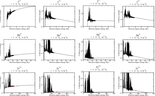
As a sample of the results, we show in Fig. 2 the collision strengths for some important transitions within the n =2 com-plex (see Del Zanna et al. 2008) for the benchmark ions in the Be-like sequence. We show four different types of transitions: dipole allowed (1−5), dipole allowed through spin-orbit mixing (1−3), a double-electron-jump Born transition (1−9), and a forbidden one (1−4). The collision strengths present the usual structure, a resonance region for the energies which correspond to transitions between the calculated levels, and a regular back-ground. For dipole allowed transitions, the collision strength di-verges logarithmically as the energy tends to infinity, while for non dipole allowed transitions it tends to a constant and for for-bidden transitions the collision strength tends to zero as E−2 in the infinite energy limit.
0 2 4 6 8 10
Electron impact energy (Ry)
100
101
Collision strength
C2+
1 - 5 2s2 1S0 - 2s 2p 1P1
0 2 4 6 8 10
Electron impact energy (Ry)
10-2
10-1
100
Collision strength
C2+
1 - 3 2s2 1S0 - 2s 2p
3
P1
0 2 4 6 8 10
Electron impact energy (Ry)
10-1
100
Collision strength
C2+
1 - 9 2s2 1S0 - 2p2
1
D2
0 2 4 6 8 10
Electron impact energy (Ry)
10-2
10-1
100
Collision strength
C2+
1 - 4 2s2 1S0 - 2s 2p
3
P2
0 10 20 30 40 50 60 70
Electron impact energy (Ry)
100
101
Collision strength
Mg8+
1 - 5 2s2 1S0 - 2s 2p 1P1
0 10 20 30 40 50 60 70
Electron impact energy (Ry)
10-3
10-2
10-1
100
Collision strength
Mg8+
1 - 3 2s2 1S0 - 2s 2p
3
P1
0 10 20 30 40 50 60 70
Electron impact energy (Ry)
10-2
10-1
100
Collision strength
Mg8+
1 - 9 2s2 1S
0 - 2p
2 1
D
2
0 10 20 30 40 50 60 70
Electron impact energy (Ry)
10-2
10-1
100
Collision strength
Mg8+
1 - 4 2s2 1S0 - 2s 2p
3
P2
0 100 200 300 400
Electron impact energy (Ry)
10-1
100
101
Collision strength
Fe22+
1 - 5 2s2 1S0 - 2s 2p
1
P1
0 100 200 300 400
Electron impact energy (Ry)
10-2
10-1
100
Collision strength
Fe22+
1 - 3 2s2 1S0 - 2s 2p
3
P1
0 100 200 300 400
Electron impact energy (Ry)
10-3
10-2
10-1
100
Collision strength
Fe22+
1 - 9 2s2 1S0 - 2p2 1D2
0 100 200 300 400
Electron impact energy (Ry)
10-3
10-2
10-1
100
Collision strength
Fe22+
1 - 4 2s2 1S0 - 2s 2p
3
[image:5.595.46.552.58.371.2]P2
Fig. 2. Electron-impact excitation collision strengths versus the impact energy for some selected transitions within the n =2 complex for the benchmark ions. Full line: present R-matrix work;¤: distorted wave results of Bhatia&Mason (1981). (Colour online)
.
while the impact energy increases as a factor z2. The height of the resonances increases as a factor z2too, with respect to the background. The relative strength of the background can also increase with increasing charge due to increased spin-orbit mixing, for example, in singlet-triplet mixing. This ef-fect is clearly seen in the transition 1−3. The spin-orbit mix-ing of3P with 1P turns this transition into a dipole allowed one for iron, with corresponding asymptotic behavior, while in carbon (with a much lower nuclear charge) it behaves as a forbidden transition still.
For the case of Fe22+, we show also in Fig. 2 a comparison with the distorted wave results of Bhatia & Mason (1981). While there is good agreement between the distorted wave collision strengths and the background R-matrix ones, the omission of resonances by the former method can give rise to significant differences in Maxwellian rate coefficients for some transitions. Chidichimo et al. (1999, 2005) compared their R-matrix results for ground-state transitions to levels of n = 2 and 3 with the distorted wave ones of Bhatia &
Mason (1981) and found differences of up to a factor of two and∼30%, respectively, at 107K.
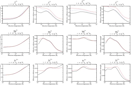
Fig. 3 shows our Maxwell integrated effective collision strengths for the same transitions as shown in Fig. 2. The fig-ure also shows a comparison with the previous benchmark cal-culations: Berrington et al. (1985); Del Zanna et al. (2008); Chidichimo et al. (2005); Mitnik et al. (2003). The Mitnik et al. (2003) calculation included Laguerre pseudostates in the close-coupling expansion. It was performed in LS -close-coupling and a di-rect comparison without further recoupling can only be made for transitions which involve a singlet state (or an S-state),
fol-lowing a generalization of Burgess et al. (1970), equation (99) etc. For the singlet–triplet transitions, level resolution can be de-termined simply by multiplying the effective collision strength by the fractional statistical weight of the level. The inclusion of pseudostates gives a difference of less than 10% compared to calculations without them.
For low temperatures, the center of the Maxwellian envelope lies on the resonance region, so such temperatures are quite sen-sitive to the good description of the resonances, if the impact energy mesh is fine enough. Thus, we have carried out a conver-gence study of the effective collision strengths at low tempera-ture and we have checked that the fine mesh step used is suffi -cient for the ions under consideration. Overall, excellent agree-ment with previous calculations is found. This indicates that res-onance excitation due to the extra configurations in our extended target does not produce significant enhancements for the n=2 transitions. The transition (1−3) shows when the spin orbit gives an important contribution. For carbon and magnesium this tran-sition behaves as forbidden for temperatures of physical interest, but for iron it shows dipole behavior.
104 105 106 107
Electron temperature (K)
0 2 4 6 8 10 12 14
Effective collision strength
C2+
1 - 5 2s2 1S0 - 2s 2p 1P1
104 105 106 107
Electron temperature (K)
0 0.1 0.2 0.3 0.4
Effective collision strength
C2+
1 - 3 2s2 1S0 - 2s 2p
3
P1
104 105 106 107
Electron temperature (K)
0 0.1 0.2 0.3 0.4 0.5
Effective collision strength
C2+
1 - 9 2s2 1S 0 - 2p
2 1 D
2
104 105 106 107
Electron temperature (K)
0 0.1 0.2 0.3 0.4 0.5 0.6
Effective collision strength
C2+
1 - 4 2s2 1S0 - 2s 2p
3
P2
104 105 106 107 108
Electron temperature (K)
0 1 2 3 4
Effective collision strength
Mg8+
1 - 5 2s2 1S
0 - 2s 2p
1
P
1
104 105 106 107 108
Electron temperature (K)
0 0.01 0.02 0.03 0.04 0.05 0.06
Effective collision strength
Mg8+
1 - 3 2s2 1S0 - 2s 2p 3P1
104 105 106 107 108
Electron temperature (K)
0 0.005 0.01 0.015 0.02 0.025
Effective collision strength
Mg8+
1 - 9 2s2 1S
0 - 2p
2 1
D
2
104 105 106 107 108
Electron temperature (K)
0 0.02 0.04 0.06 0.08 0.1
Effective collision strength
Mg8+
1 - 4 2s2 1S0 - 2s 2p 3P2
105 106 107 108 109
Electron temperature (K)
0 0.2 0.4 0.6 0.8
Effective collision strength
Fe22+
1 - 5 2s2 1S0 - 2s 2p
1
P1
105 106 107 108 109
Electron temperature (K)
0 0.005 0.01 0.015 0.02
Effective collision strength
Fe22+
1 - 3 2s2 1S0 - 2s 2p 3P1
105 106 107 108 109
Electron temperature (K)
0 0.0004 0.0008 0.0012 0.0016
Effective collision strength
Fe22+
1 - 9 2s2 1S0 - 2p2 1D2
105 106 107 108 109
Electron temperature (K)
0 0.005 0.01 0.015
Effective collision strength
Fe22+
[image:6.595.47.551.57.386.2]1 - 4 2s2 1S0 - 2s 2p 3P2
Fig. 3. Electron-impact excitation effective collision strengths versus the electron temperature for some selected transitions and targets, as in Fig. 2. Full line: present work; dashed line: C2+Berrington et al. (1989), Mg8+Del Zanna et al. (2008), and Fe22+Chidichimo et al. (2005); dotted line:
C2+Mitnik et al. (2003). (Colour online.)
Effective collision strengths for weak transitions can have a considerable contribution from resonances at lower tem-peratures. The present close-coupling expansion is larger than those used in previous (non-pseudo-state) R-matrix works, especially those which only expanded up to n =
3. Consequently, we expect a larger resonance enhance-ment compared to those works, and we illustrate a case in Fig. 4. There we compare our effective collision strengths for the 2s2 1S
0 −2s3p3P1 transition in Ne6+ with the LS -plus-algebraic recoupling R-matrix results of Ramsbottom et al. (1995). At low temperatures our results display a much larger resonance enhancement, compared to those of Ramsbottom et al. (1995), while at high temperatures we see the influence of spin-orbit mixing turning the high-energy/temperature tail from a forbidden to weak dipole-allowed one.
Fig. 5 shows the effective collision strengths for some se-lected transitions of P11+. Be-like P11+has not been calculated before using the R-matrix method or a DW method, and the data currently used for diagnostic modeling within the CHIANTI database are interpolated ones from Keenan (1988). In this fig-ure we show the same set of transitions as in Fig. 3. The double-electron-jump (1−9) shows differences between the R-matrix calculations and the interpolated data, and in the spin-changing transition (1−3) the discrepancy is quite large. Asymptotically, the transition 1−3 behaves as a dipole one through spin-orbit mixing, as discussed earlier. But, algebraic recoupling only of
LS -coupling data does not include such mixing and it (1−3)
10
410
510
610
710
8Electron temperature (K)
0
0.01
0.02
0.03
0.04
Effective collision strength
Ne
6+
[image:6.595.305.557.445.654.2]1 - 15 2s
2 1S
0- 2s 3p
3P
1Fig. 4. Electron-impact excitation effective collision strengths versus the electron temperature for transition 1−15 2s2 1S
0 −2s3p3P1 of
Ne6+. Full line: present work; dashed line: Data from Ramsbottom et al.
(1995). (Colour online).
105 106 107 108
Electron temperature (K)
0 0.5 1 1.5 2 2.5
Effective collision strength
P11+
1 - 5 2s2 1S0 - 2s2p 1P1
105 106 107 108
Electron temperature (K)
0 0.1 0.2 0.3 0.4
Effective collision strength
P11+
1 - 3 2s2 1S 0 - 2s2p
3 P
1
105 106 107 108
Electron temperature (K)
0 0.002 0.004 0.006 0.008 0.01
Effective collision strength
P11+
1 - 9 2s2 1S
0 - 2p
2 1
D
2
105 106 107 108
Electron temperature (K)
0 0.01 0.02 0.03 0.04 0.05
Effective collision strength
P11+
[image:7.595.52.553.57.160.2]1 - 4 2s2 1S0 - 2s2p 3P2
Fig. 5. Electron-impact excitation effective collision strengths versus the electron temperature for some selected transitions of P11+. Full line:
present work; dashed line: interpolated data from Keenan (1988). (Colour online).
Table 2. Comparison of (scaled) infinite energy limit points for
some dipole (4S/3) and allowed (Born) transitions in Fe22+. Previous:
Chidichimo et al. (2005). A (B) denotes A×10B.
Transition ΩPresent work ΩPrevious 1−12 1.732 (−2) 1.640 (−2) 1−18 2.296 (−4) 2.115 (−4) 1−20 4.785 (−2) 4.784 (−2) 1−26 7.889 (−5) 9.233 (−5) 1−28 6.840 (−6) 5.990 (−6) 1−32 2.725 (−5) 2.413 (−5) 1−35 9.170 (−5) 1.099 (−4) 1−37 1.763 (−4) 2.369 (−4) 1−40 9.745 (−6) 8.954 (−6) 1−44 4.097 (−5) 3.779 (−5) 1−45 1.594 (−4) 1.548 (−4) 1−48 3.478 (−3) 2.995 (−3) 1−54 6.394 (−5) 6.059 (−5) 1−56 7.296 (−3) 7.435 (−3) 1−58 9.053 (−5) 7.548 (−5) 1−60 2.611 (−3) 2.573 (−3) 1−65 3.928 (−6) 4.455 (−6) 1−66 1.528 (−5) 1.050 (−5) 1−69 1.036 (−5) 8.712 (−6) 1−73 4.017 (−5) 3.922 (−5) 1−75 5.630 (−6) 5.013 (−6) 1−78 2.107 (−6) 2.314 (−6) 1−79 5.146 (−6) 6.350 (−6) 1−84 1.638 (−6) 1.230 (−6) 1−85 4.304 (−5) 2.907 (−5) 1−90 1.757 (−7) 1.864 (−7) 1−91 1.356 (−5) 4.049 (−5) 1−94 8.444 (−6) 7.422 (−6) 1−95 2.408 (−5) 1.964 (−5) 1−98 4.034 (−5) 1.338 (−5)
We close this section with a note of caution: we have shown only a selection of transitions and when the totality of excita-tions plus-cascade are modeled then Del Zanna et al. (2008) has shown that significant problems can arise on using interpolated data.
5. Conclusions
We have presented a complete data set of ICFT R-Matrix cal-culations of electron-impact excitation of all ions in the Be-like isoelectronic sequence from B+to Zn26+. We have shown a se-lected set of collision strengths and effective collision strengths
for some important n = 2 transitions and ions, finding good agreement with previous similar calculations. The present work expands the previous ones Del Zanna et al. (2008); Chidichimo et al. (2003); Chidichimo et al. (2005) for Be-like Mg, Fe and Ni, by significantly increasing the orbitals in the basis set.
The present data set constitutes a significant improvement over previous available data for many ions in the Be-like se-quence, which was based upon interpolated data. With our basis set emission lines including from cascade effects from levels up to n=7 can be predicted. With the present data, emission lines from Be-like ions can reliably be used for diagnostics of tem-perature and density of astrophysical and fusion plasmas. The atomic data are made available at our APAP network web page2. They will also be uploaded into the OPEN-ADAS3 and CHI-ANTI4databases.
Work is in progress to expand the method to other isoelec-tronic sequences, in particular, the Mg-like, which is similar to this one in the sense that it consist of a closed n-shell plus two electrons.
Acknowledgements. The present work was funded by STFC (UK) through the
University of Strathclyde UK APAP network grant ST/J000892/1 and the Uni-versity of Cambridge DAMTP astrophysics grant.
References
Audard, M. 2003, Advances in Space Research, 32, 927 Badnell, N. R. 2011, Comput. Phys. Commun., 182, 1528 Badnell, N. R. & Griffin, D. C. 1999, J. Phys. B, 32, 2267 Badnell, N. R. & Griffin, D. C. 2001, J. Phys. B, 34, 681
Badnell, N. R., Griffin, D. C., & Mitnik, D. M. 2003, Journal of Physics B: Atomic, Molecular and Optical Physics, 36, 1337
Berrington, K. A., Burke, P. G., Dufton, P. L., & Kingston, A. E. 1985, Atomic Data and Nuclear Data Tables, 33, 195
Berrington, K. A., Burke, V. M., Burke, P. G., & Scialla, S. 1989, Journal of Physics B: Atomic, Molecular and Optical Physics, 22, 665
Berrington, K. A., Eissner, W. B., & Norrington, P. H. 1995, Comput. Phys. Commun., 92, 290
Bhatia, A. K. & Landi, E. 2007, At. Data Nucl. Data Tables, 93, 275 Bhatia, A. K. & Mason, H. E. 1981, Astron. Astrophys., 103, 324
Burgess, A. 1974, Journal of Physics B: Atomic and Molecular Physics, 7, L364 Burgess, A., Chidichimo, M. C., & Tully, J. A. 1997, J. Phys. B, 30, 33 Burgess, A., Hummer, D. G., & Tully, J. A. 1970, Philos. Trans. R. Soc. London,
Ser. A, 266, 225
Burgess, A. & Tully, J. A. 1992, Astron. Astrophys., 254, 436
Chidichimo, M. C., Badnell, N. R., & Tully, J. A. 2003, A&A, 401, 1177 Chidichimo, M. C., Del Zanna, G., Mason, H. E., et al. 2005, Astron. Astrophys.,
430, 331
Chidichimo, M. C., Zeman, V., Tully, J. A., & Berrington, K. A. 1999, Astron. Astrophys. Suppl. Ser., 137, 175
Del Zanna, G. & Mason, H. E. 2005, Astron. Astrophys., 432, 1137
2 http://www.apap-network.org 3 http://open.adas.ac.uk
[image:7.595.75.255.250.604.2]Del Zanna, G., Rozum, I., & Badnell, N. R. 2008, Astron. Astrophys., 487, 1203 Dere, K. P. 1978, Astrophys. J., 221, 1062
Dere, K. P., Landi, E., Mason, H. E., Monsignori-Fossi, B. C., & Young, P. R. 1997, Astron. Astrophys. Suppl. Ser., 125, 149
Dufton, P. L., Kingston, A. E., & Scott, N. S. 1983, J. Phys. B., 16, 3053 Eissner, W. M., Jones, M., & H, N. 1974, Comput. Phys Commun., 8, 270 Griffin, D. C., Badnell, N. R., & Pindzola, M. S. 1998, J. Phys. B, 31, 3713 Hummer, D. G., Berrington, K. A., Eissner, W., et al. 1993, Astron. Astrophys.,
279, 298
Inoue, T., Nakai, M., Tanaka, A., et al. 2001, Plasma Phys. Control. Fusion, 43, L9
Keenan, F. P. 1988, Physica Scripta, 37, 57
Keenan, F. P., Berrington, K. A., Burke, P. G., Dufton, P. L., & Kingston, A. E. 1986, Phys. Scr., 34, 216
Li, F., Liang, G. Y., Bari, M. A., & Zhao, G. 2013, Astron. Astrophys., 556, A32 Liang, G. Y., Badnell, N. R., & Zhao, G. 2012, Astron. Astrophys., 547, A87 Martin, W. C. & Zalubas, R. 1980, Journal of Physical and Chemical Reference
Data, 9, 1
Mitnik, D. M., Griffin, D. C., Ballance, C. P., & Badnell, N. R. 2003, Journal of Physics B: Atomic, Molecular and Optical Physics, 36, 717
Moore, C. E. 1993, in Tables of Spectra of Hydrogen, Carbon, Nitrogen and Oxygen Atoms and Ions, ed. J. W. Gallacher, CRC Series in Evaluated Data in Atomic Physics (CRC Press)
Neupert, W. M., Gates, W., Swartz, M., & Young, R. 1967, Astrophys. J., 149, L79
Ramsbottom, C. A., Berrington, K. A., & Bell, K. L. 1994a, J. Phys. B, 27, L811 Ramsbottom, C. A., Berrington, K. A., & Bell, K. L. 1995, At. Data Nucl. Data
Tables, 61, 105
Ramsbottom, C. A., Berrington, K. A., Hibbert, A., & Bell, K. L. 1994b, Phys. Scr., 50, 246
Sampson, D. H., Goett, S. J., & Clark, R. E. H. 1984, Atomic Data and Nuclear Data Tables, 30, 125
Sandlin, G. D., Bartoe, J.-D. F., Tousey, R., & Van Hoosier, M. E. 1986, Astro-phys. J. Suppl. Ser., 61, 801
Sugar, J. & Corliss, C. 1985, J. Phys. Chem. Ref. Data, 1
Summers, H. P., Dickson, W. J., Boileau, A., et al. 1992, Plasma Physics and Controlled Fusion, 34, 325
Tachiev, G. & Fischer, C. F. 1999, J. Phys. B, 32, 5805
Vernazza, J. E. & Reeves, E. M. 1978, Astrophys J. Suppl, 37, 485
Wilhelm, K., Marsch, E., Dwivedi, B. N., et al. 1998, Astrophys. J., 500, 1023 Witthoeft, M. C., Whiteford, A. D., & Badnell, N. R. 2007, J. Phys. B: At. Mol.
Opt. Phys., 40, 2969
Table 3. Thomas-Fermi-Dirac-Amaldi potential scaling factors used incalculation.
Ion 1s 2s 2p 3s 3p 3d 4s 4p 4d 4f
5s 5p 5d 5f 5g 6s 6p 6d 7s 7p 7d
B+ 1.39653 1.46875 1.43661 1.19439 1.14553 1.29613 1.19203 1.13186 1.29804 1.45128
1.19330 1.12751 1.30168 1.45196 1.57425 1.19540 1.12564 1.30678 1.19849 1.12477 1.31345 C2+ 1.41290 1.49099 1.43422 1.20193 1.13345 1.27955 1.20122 1.12308 1.28131 1.43825
1.20319 1.11983 1.28608 1.44185 1.57035 1.20542 1.11806 1.29188 1.20938 1.11667 1.29554 N3+ 1.43000 1.50845 1.43689 1.21092 1.13140 1.27332 1.21098 1.12277 1.27607 1.43341
1.21343 1.12037 1.28215 1.43924 1.55457 1.21659 1.11834 1.28456 1.22184 1.11739 1.28733 O4+ 1.44986 1.52368 1.44080 1.22007 1.13315 1.27102 1.22074 1.12656 1.27530 1.44272
1.22378 1.12262 1.27931 1.44190 1.54473 1.22792 1.12112 1.28112 1.23339 1.11910 1.28155 F5+ 1.47345 1.53823 1.44532 1.23007 1.13634 1.27176 1.23140 1.12941 1.27676 1.45042
1.23579 1.12547 1.27851 1.44190 1.58397 1.23970 1.12653 1.27874 1.24668 1.12543 1.27878 Ne6+ 1
.50238 1.61111 1.44991 1.24485 1.13968 1.27306 1.24651 1.13170 1.27109 1.45896
1.25340 1.12866 1.27787 1.46014 0.17214 1.25114 1.12823 1.27534 1.25978 1.13215 1.29033 Na7+ 1
.53841 1.56981 1.45496 1.25454 1.14548 1.27582 1.25766 1.14271 1.27844 1.45585
1.25613 1.13208 1.27826 1.49334 1.69385 1.26776 1.16973 1.28085 1.28134 1.13540 1.30630 Mg8+ 1.24000 1.59549 1.46744 1.27389 1.15697 1.27971 1.27754 1.15316 1.28140 2.06981
1.28021 1.14906 1.27926 1.50322 1.89909 1.28950 1.14724 1.29386 1.28025 1.15310 1.31404 Al9+ 1.25000 1.61669 1.47329 1.29225 1.16420 1.28342 1.29693 1.16044 1.28450 1.96809
1.29904 1.17984 1.28149 1.52430 1.85742 1.30930 1.15922 1.30526 1.30787 1.16520 1.32541 Si10+ 1.27000 1.63993 1.48096 1.31345 1.17269 1.28795 1.31899 1.16446 1.28771 1.50502
1.32219 1.16996 1.29524 1.52410 1.86078 1.33213 1.17292 1.31636 1.33749 1.17722 1.33820 P11+ 1.29000 1.66698 1.48863 1.33792 1.18239 1.29330 1.34453 1.17405 1.29175 1.52229
1.32916 1.17753 1.30630 1.54557 1.86065 1.36058 1.17768 1.32799 1.35421 1.18970 1.34597 S12+ 1.32000 1.69798 1.49820 1.36619 1.19385 1.29928 1.37362 1.18607 1.29705 1.54291
1.37509 1.18607 1.31273 1.54252 1.85894 1.40135 1.19959 1.36643 1.38328 1.20349 1.35765 Cl13+ 1
.34000 1.73414 1.51315 1.39842 1.20570 1.30618 1.40687 1.41009 1.30748 1.56630
1.44054 1.20384 1.33685 1.60963 1.85107 1.38976 1.21181 1.35402 1.41456 1.21988 1.36876 Ar14+ 1.38000 1.77486 1.51919 1.43674 1.22246 1.31414 1.44543 1.21480 1.32216 1.57071
1.44720 1.21869 1.36034 1.59897 1.77197 1.42508 1.22830 1.36468 1.45103 1.23554 1.38174 K15+ 1.42000 1.82173 1.53065 1.47991 1.23087 1.32155 1.48906 1.23105 1.33713 1.59368
1.48858 1.24032 1.38104 1.62515 2.10990 1.48167 1.24772 1.37835 1.49367 1.25383 1.39537 Ca16+ 1.47000 1.87511 1.54387 1.52883 1.24783 1.32959 1.53787 1.25088 1.35215 1.61528
1.53483 1.26078 1.37265 1.65110 2.12513 1.53123 1.26716 1.39392 1.54165 1.27363 1.41068 Sc17+ 1.53000 1.93788 1.59589 1.75156 1.26621 1.33795 1.59469 1.27257 1.36750 1.63587
1.58985 1.28349 1.39183 1.67574 2.15051 1.58759 1.29120 1.40896 1.59725 1.29707 1.42576 Ti18+ 1.60000 2.00584 1.57603 1.65114 1.27591 1.35026 1.65665 1.29754 1.38595 1.65776
1.65154 1.30781 1.41023 1.70303 2.19714 1.65227 1.31642 1.42776 1.66059 1.32362 1.44441 V19+ 1.68000 2.08529 1.59641 1.72470 1.36143 1.36267 1.72709 1.32503 1.40464 1.68328
1.72037 1.33534 1.42895 1.73176 2.23923 1.68904 1.34592 1.44648 1.73785 1.33680 1.46407 Cr20+ 1.79000 2.17707 1.61657 1.80606 1.33031 1.37636 1.80500 1.35470 1.42787 1.70784
1.79735 1.36558 1.44939 1.76243 2.23933 1.77710 1.37646 1.46636 1.84642 1.37410 1.48713 Mn21+ 1.92000 2.28271 1.63986 1.89840 1.35947 1.39912 1.90077 1.38817 1.43396 1.73446
1.88281 1.39830 1.47158 1.79320 2.30111 1.86717 1.39472 1.49170 1.77849 1.39979 1.50936 Fe22+ 2.09000 2.40609 1.66339 2.00074 1.39088 1.41977 1.98780 1.42379 1.46599 1.76469
1.97794 1.43521 1.49892 1.82733 2.37774 1.96099 1.43770 1.51479 1.92026 1.44292 1.53397 Co23+ 2.33000 2.55047 1.69200 2.11526 1.42494 1.44148 2.09657 1.46324 1.48980 1.79380
2.08337 1.47543 1.52191 1.86205 2.38007 2.06500 1.50871 1.54053 2.03551 1.51276 1.56093 Ni24+ 2.66000 2.72055 1.72256 2.24298 1.46199 1.46465 2.21669 1.50708 1.51495 1.82611
2.20013 1.55010 1.54587 1.89817 2.45661 2.18012 1.55583 1.56840 2.15389 1.55986 1.58994 Cu25+ 3.16000 2.92546 1.76525 2.38879 1.50301 1.48887 2.35148 1.55565 1.54173 1.85563
2.33131 1.59550 1.57404 1.93698 2.52032 2.30874 1.60920 1.59817 2.28313 1.61318 1.63090 Zn26+ 4
.03000 3.21931 1.79979 2.54953 1.54609 1.51586 2.49745 1.60297 1.57155 1.88843
Table 4. C2+target levels.
i Conf. Level Eth( %) ENIST ECHIANTI( %) i Conf. Level Eth( %) ENIST ECHIANTI(%)
1 2s2 1S
0 0.( −) 0. 0.( −) 50 2p 3d 3Fo4 332279.(0.4) 333447. −(−)
2 2s 2p 3Po
0 53715.(2.6) 52367. 52432.(0.1) 51 2p 3p
1D
2 333829.(0.2) 333118. −(−)
3 2s 2p 3Po
1 53750.(2.6) 52391. 52432.(0.1) 52 2p 3d
3Do
1 335540.(0.6) 337656. −(−)
4 2s 2p 3Po
2 53820.(2.6) 52447. 52432.(0.0) 53 2p 3d
3Do
2 335554.(0.6) 337669. −(−)
5 2s 2p 1Po
1 110046.(7.5) 102352. 103252.(0.9) 54 2p 3d
3Do
3 335575.(0.6) 337688. −(−)
6 2p2 3P
0 141612.(3.0) 137426. 138247.(0.6) 55 2s 5s 1S0 335888.(0.8) 338514. −(−)
7 2p2 3P
1 141646.(3.0) 137454. 138247.(0.6) 56 2s 5s 3S1 336531.(1.0) 339935. −(−)
8 2p2 3P
2 141715.(3.1) 137502. 138247.(0.5) 57 2p 3d 3Po2 337994.(0.6) 340102. −(−)
9 2p2 1D
2 154426.(5.9) 145876. 146422.(0.4) 58 2p 3d 3Po1 338014.(0.6) 340128. −(−)
10 2p2 1S
0 194713.(6.7) 182520. 185094.(1.4) 59 2p 3d 3Po0 338024.(0.6) 340142. −(−)
11 2s 3s 3S
1 235036.(1.3) 238213. 237164.(0.4) 60 2s 5f 1Fo3 340059.(2.5) 348860. −(−)
12 2s 3s 1S
0 244899.(0.9) 247170. 246492.(0.3) 61 2s 5p 1Po1 340665.(0.8) 343258. −(−)
13 2s 3p 1Po
1 256774.(0.8) 258931. 258223.(0.3) 62 2s 5p
3Po
2 341178.(0.9) 344233. −(−)
14 2s 3p 3Po
0 256810.(1.1) 259706. 258881.(0.3) 63 2s 5p
3Po
1 341187.(0.9) 344236. −(−)
15 2s 3p 3Po
1 256818.(1.1) 259711. 258881.(0.3) 64 2s 5p
3Po
0 341191.(0.9) 344239. −(−)
16 2s 3p 3Po
2 256829.(1.1) 259724. 258881.(0.3) 65 2s 5d
3D
1 342134.(1.0) 345497. −(−)
17 2s 3d 3D
1 267262.(1.0) 270011. 268922.(0.4) 66 2s 5d 3D2 342134.(1.0) 345497. −(−)
18 2s 3d 3D
2 267264.(1.0) 270012. 268922.(0.4) 67 2s 5d 3D3 342135.(1.0) 345497. −(−)
19 2s 3d 3D
3 267268.(1.0) 270015. 268922.(0.4) 68 2s 5g 3G3 343014.(1.0) 346579. −(−)
20 2s 3d 1D
2 275338.(0.4) 276483. 276308.(0.1) 69 2s 5g 3G4 343015.(1.0) 346579. −(−)
21 2s 4s 3S
1 306319.(1.0) 309457. −( −) 70 2s 5g 3G5 343015.(1.0) 346579. −(−)
22 2p 3s 3Po
0 306368.(0.6) 308217. −( −) 71 2s 5g
1G
4 343015.(1.0) 346579. −(−)
23 2p 3s 3Po
1 306403.(0.6) 308249. −( −) 72 2s 5d
1D
2 343749.(0.8) 346658. −(−)
24 2p 3s 3Po
2 306475.(0.6) 308317. −( −) 73 2s 5f
3Fo
2 343914.(0.9) 347152. −(−)
25 2p 3s 1Po
1 308394.(0.5) 310006. −( −) 74 2s 5f
3Fo
3 343916.(0.9) 347153. −(−)
26 2s 4s 1S
0 308465.(1.0) 311722. −( −) 75 2s 5f 3Fo4 343920.(0.9) 347155. −(−)
27 2s 4p 3Po
0 314505.(1.0) 317794. −( −) 76 2p 3p
1S
0 346252.(0.3) 345095. −(−)
28 2s 4p 3Po
1 314508.(1.0) 317797. −( −) 77 2p 3d
1Po
1 346391.(0.1) 346713. −(−)
29 2s 4p 3Po
2 314512.(1.0) 317801. −( −) 78 2p 3d
1Fo
3 348219.(2.0) 341371. −(−)
30 2p 3p 1P
1 317694.(0.6) 319720. −( −) 79 2s 6s 3S1 351405.(1.0) 354858. −(−)
31 2s 4d 3D
1 318501.(0.9) 321411. −( −) 80 2s 6s 1S0 352937.( −) − −(−)
32 2s 4d 3D
2 318507.(0.9) 321427. −( −) 81 2s 6p 3Po0 353549.(1.0) 357049. −(−)
33 2s 4d 3D
3 318517.(0.9) 321450. −( −) 82 2s 6p 3Po1 353550.(1.0) 357050. −(−)
34 2s 4f 3Fo
2 318840.(1.0) 322004. −( −) 83 2s 6p
3Po
2 353551.(1.0) 357051. −(−)
35 2s 4f 3Fo
3 318846.(1.0) 322010. −( −) 84 2s 6p
1Po
1 353819.(0.9) 357110. −(−)
36 2s 4f 3Fo
4 318853.(1.0) 322018. −( −) 85 2s 6d
3D
1 354636.(1.0) 358098. −(−)
37 2s 4f 1Fo
3 319376.(1.0) 322702. −( −) 86 2s 6d
3D
2 354636.(1.0) 358098. −(−)
38 2p 3p 3D
1 321171.(0.6) 323077. −( −) 87 2s 6d 3D3 354637.(1.0) 358098. −(−)
39 2p 3p 3D
2 321206.(0.6) 323101. −( −) 88 2s 6d 1D2 355514.(0.9) 358733. −(−)
40 2p 3p 3D
3 321260.(0.6) 323140. −( −) 89 2s 7s 3S1 360131.(1.0) 363613. −(−)
41 2s 4d 1D
2 321734.(0.8) 324212. −( −) 90 2s 7s 1S0 360660.( −) − −(−)
42 2s 4p 1Po
1 321867.(0.2) 322404. −( −) 91 2s 7p
3Po
0 361434.( −) − −(−)
43 2p 3p 3S
1 325461.(0.6) 327278. −( −) 92 2s 7p 3Po1 361434.( −) − −(−)
44 2p 3p 3P
0 328376.(0.4) 329685. −( −) 93 2s 7p 3Po2 361435.( −) − −(−)
45 2p 3p 3P
1 328399.(0.4) 329706. −( −) 94 2s 7p 1Po1 361466.(0.9) 364896. −(−)
46 2p 3p 3P
2 328442.(0.4) 329744. −( −) 95 2s 7d 3D1 362131.(1.0) 365638. −(−)
47 2p 3d 1Do
2 330524.(0.7) 332691. −( −) 96 2s 7d
3D
2 362131.(1.0) 365638. −(−)
48 2p 3d 3Fo
2 332208.(0.4) 333387. −( −) 97 2s 7d
3D
3 362132.(1.0) 365638. −(−)
49 2p 3d 3Fo
3 332238.(0.4) 333412. −( −) 98 2s 7d
1D
2 362681.(0.9) 366028. −(−)
Notes. Key: i: level index; Conf.: configuration; Level: level IC designation; Eth: theoretical level energy (cm−1), this work; ENIST: observed
energy from the NIST database and reference Moore (1993) (cm−1); E
B85: previous theoretical calculation of Berrington et al. (1985, 1989) as in
Table 5. Mg8+target levels.
i Conf. Level Eth( %) ENIST ECHIANTI( %) i Conf. Level Eth( %) ENIST ECHIANTI( %)
1 2s2 1S
0 0.( −) 0. 0.( −) 50 2s 4p 3Po1 2063734.( −) − 2064924.( −)
2 2s 2p 3Po
0 140982.(0.3) 140504. 141277.(0.6) 51 2s 4p
3Po
2 2064011.( −) − 2065186.( −)
3 2s 2p 3Po
1 142270.(0.5) 141631. 142555.(0.7) 52 2s 4p
1Po
1 2066449.(0.1) 2068680. 2067943.(0.0)
4 2s 2p 3Po
2 144920.(0.6) 144091. 145184.(0.8) 53 2s 4d
3D
1 2077595.(0.1) 2079970. 2078838.(0.1)
5 2s 2p 1Po
1 278399.(2.5) 271687. 279967.(3.0) 54 2s 4d
3D
2 2077645.(0.1) 2079970. 2078885.(0.1)
6 2p2 3P
0 369168.(0.9) 365856. 369930.(1.1) 55 2s 4d 3D3 2077720.(0.1) 2080050. 2078957.(0.1)
7 2p2 3P
1 370555.(0.9) 367159. 371306.(1.1) 56 2s 4d 1D2 2086270.(0.1) 2087890. 2087551.(0.0)
8 2p2 3P
2 373076.(1.0) 369330. 373811.(1.2) 57 2s 4f 3Fo2 2086530.( −) − 2087845.( −)
9 2p2 1D
2 413143.(2.0) 405100. 414538.(2.3) 58 2s 4f 3Fo3 2086558.( −) − 2087874.( −)
10 2p2 1S
0 513046.(2.7) 499633. 514353.(2.9) 59 2s 4f 3Fo4 2086597.( −) − 2087912.( −)
11 2s 3s 3S
1 1529401.(0.2) 1532450. 1530734.(0.1) 60 2s 4f 1Fo3 2089095.( −) − 2090438.( −)
12 2s 3s 1S
0 1555861.(0.1) 1558080. 1556824.(0.1) 61 2p 4s 3Po0 2205006.( −) − 2206147.( −)
13 2s 3p 1Po
1 1591800.(0.1) 1593600. 1593190.(0.0) 62 2p 4s
3Po
1 2205866.( −) − 2207065.( −)
14 2s 3p 3Po
0 1594402.(0.2) 1597500. 1595438.(0.1) 63 2p 4s
3Po
2 2208975.( −) − 2210045.( −)
15 2s 3p 3Po
1 1594786.(0.2) 1597500. 1595820.(0.1) 64 2p 4s
1Po
1 2213758.( −) − 2216284.( −)
16 2s 3p 3Po
2 1595382.(0.1) 1597500. 1596396.(0.1) 65 2p 4p
1P
1 2222434.( −) − 2223811.( −)
17 2s 3d 3D
1 1629120.(0.1) 1631040. 1630250.(0.0) 66 2p 4p 3D1 2225037.(0.2) 2229730. 2226363.(0.2)
18 2s 3d 3D
2 1629265.(0.1) 1631170. 1630392.(0.0) 67 2p 4p 3D2 2225527.(0.2) 2229730. 2226814.(0.1)
19 2s 3d 3D
3 1629481.(0.1) 1631320. 1630606.(0.0) 68 2p 4p 3D3 2228012.(0.1) 2229730. 2229254.(0.0)
20 2s 3d 1D
2 1655247.(0.0) 1654580. 1656673.(0.1) 69 2p 4p 3S1 2229779.( −) − 2232150.( −)
21 2p 3s 3Po
0 1708717.(0.1) 1710140. 1709859.(0.0) 70 2p 4p
3P
0 2231743.(0.2) 2235350. 2232782.(0.1)
22 2p 3s 3Po
1 1709922.(0.1) 1711250. 1711046.(0.0) 71 2p 4p
3P
1 2233367.(0.1) 2235350. 2234713.(0.0)
23 2p 3s 3Po
2 1712655.(0.1) 1713900. 1713727.(0.0) 72 2p 4p
3P
2 2234238.(0.0) 2235350. 2235180.(0.0)
24 2p 3s 1Po
1 1738200.(0.3) 1743040. 1739718.(0.2) 73 2p 4d
3Fo
2 2236868.( −) − 2238216.( −)
25 2p 3p 1P
1 1746573.(0.1) 1748120. 1747844.(0.0) 74 2p 4d 3Fo3 2238744.( −) − 2240126.( −)
26 2p 3p 3D
1 1754038.(0.1) 1755470. 1755314.(0.0) 75 2p 4d 1Do2 2239512.(0.1) 2241210. 2240728.(0.0)
27 2p 3p 3D
2 1755312.(0.1) 1756470. 1756575.(0.0) 76 2p 4p 1D2 2240645.( −) − 2241804.( −)
28 2p 3p 3D
3 1757821.(0.1) 1758970. 1759043.(0.0) 77 2p 4d 3Fo4 2240951.( −) − 2242301.( −)
29 2p 3p 3S
1 1769176.(0.1) 1770380. 1770506.(0.0) 78 2p 4d 3Do1 2244211.(0.2) 2248250. 2245305.(0.1)
30 2p 3p 3P
0 1776847.(0.1) 1778690. 1777823.(0.0) 79 2p 4d 3Do2 2244746.(0.2) 2248250. 2245924.(0.1)
31 2p 3p 3P
1 1777974.(0.0) 1778690. 1778928.(0.0) 80 2p 4f 1F3 2245713.( −) − 2247165.( −)
32 2p 3p 3P
2 1779442.(0.0) 1779990. 1780368.(0.0) 81 2p 4d 3Do3 2246210.(0.1) 2248250. 2247192.(0.0)
33 2p 3d 3Fo
2 1784961.( −) − 1786049.( −) 82 2p 4f
3F
4 2246289.( −) − 2247857.( −)
34 2p 3d 3Fo
3 1786999.( −) − 1788095.( −) 83 2p 4f
3F
3 2246295.( −) − 2247532.( −)
35 2p 3d 1Do
2 1788309.(0.1) 1789640. 1789216.(0.0) 84 2p 4f
3F
2 2246487.( −) − 2247527.( −)
36 2p 3d 3Fo
4 1789052.( −) − 1790110.( −) 85 2p 4p
1S
0 2246795.( −) − 2256277.( −)
37 2p 3p 1D
2 1797843.(0.1) 1795870. 1799156.(0.2) 86 2p 4d 3Po2 2247691.(0.1) 2249450. 2249335.(0.0)
38 2p 3d 3Do
1 1806157.(0.1) 1807320. 1807101.(0.0) 87 2p 4d
3Po
1 2248163.(0.1) 2249970. 2249955.(0.0)
39 2p 3d 3Do
2 1806711.(0.1) 1807860. 1807645.(0.0) 88 2p 4d
3Po
0 2248402.(0.1) 2249970. 2250287.(0.0)
40 2p 3d 3Do
3 1807763.(0.1) 1808860. 1808678.(0.0) 89 2p 4f
3G
3 2249196.( −) − 2251070.( −)
41 2p 3d 3Po
2 1814627.(0.0) 1815220. 1815554.(0.0) 90 2p 4f
3G
4 2249537.( −) − 2251533.( −)
42 2p 3d 3Po
1 1815504.(0.0) 1816210. 1816418.(0.0) 91 2p 4f
3G
5 2250337.( −) − 2252907.( −)
43 2p 3d 3Po
0 1815952.(0.0) 1816730. 1816859.(0.0) 92 2p 4f
1G
4 2251731.( −) − 2254126.( −)
44 2p 3p 1S
0 1829350.( −) − 1831807.( −) 93 2p 4f 3D3 2253098.( −) − 2254413.( −)
45 2p 3d 1Fo
3 1837205.(0.1) 1834690. 1839246.(0.2) 94 2p 4f
3D
2 2253641.( −) − 2254676.( −)
46 2p 3d 1Po
1 1842786.(0.1) 1841560. 1844360.(0.2) 95 2p 4f
3D
1 2254628.( −) − 2255643.( −)
47 2s 4s 3S
1 2038676.( −) − 2040211.( −) 96 2p 4f 1D2 2255803.( −) − 2256864.( −)
48 2s 4s 1S
0 2048829.( −) − 2050281.( −) 97 2p 4d 1Fo3 2256381.(0.0) 2256570. 2259361.(0.1)
49 2s 4p 3Po
0 2063614.( −) − 2064808.( −) 98 2p 4d
1Po
1 2258053.(0.0) 2258310. 2260557.(0.1)
Notes. Key: i: level index; Conf.: configuration; Level: level IC designation; Eth: theoretical level energy (cm−1), this work; ENIST: observed energy
from the NIST data basis and reference Martin & Zalubas (1980) (cm−1); E
CHIANTI: previous theoretical calculation by Del Zanna et al. (2008) %: