The Expectation Hypothesis of the Term Structure of Very Short-Term Rates: Statistical Tests and Economic Value

      

City, University of London Institutional Repository

Citation:

Corte, P. D., Sarno, L. and Thornton, D. (2008). The Expectation Hypothesis of the Term Structure of Very Short-Term Rates: Statistical Tests and Economic Value. Journal of Financial Economics, 89(1), pp. 158-174. doi: 10.1016/j.jfineco.2007.08.002

This is the accepted version of the paper.

This version of the publication may differ from the final published

version.

Permanent repository link:

http://openaccess.city.ac.uk/13623/

Link to published version:

http://dx.doi.org/10.1016/j.jfineco.2007.08.002

Copyright and reuse: City Research Online aims to make research

outputs of City, University of London available to a wider audience.

Copyright and Moral Rights remain with the author(s) and/or copyright

holders. URLs from City Research Online may be freely distributed and

linked to.

Journal of Financial Economics 00 (0000) 000-000

The expectation hypothesis of the term structure of very short-term

rates: statistical tests and economic value

Pasquale Della Corte

a

, Lucio Sarno

a,b,c*

, Daniel L. Thornton

d

a

Finance Group, Warwick Business School, University of Warwick, Coventry CV4 7AL, UK

b

Fixed Income and FX Team, AXA Investment Managers, 7 Newgate St., London EC1A 7NX, UK

c

Centre for Economic Policy Research, 90-98 Goswell Road, London EC1V 7RR, UK

d

Research Division, Federal Reserve Bank of St. Louis, PO Box 442, St. Louis MO 63166, USA

Received 30 November 2006; received in revised format 16 July 2007; accepted 2 August 2007

Abstract

This paper reexamines the validity of the expectation hypothesis (EH) of the term

structure of US repo rates ranging in maturity from overnight to three months. We

extend the work of Longstaff (2000b) in two directions: (1) we implement statistical tests

designed to increase test power in this context; (2) more important, we assess the

economic value of departures from the EH based on criteria of profitability and economic

significance in the context of a simple trading strategy. The EH is rejected throughout the

term structure examined on the basis of the statistical tests. However, the results of our

economic analysis are favorable to the EH, suggesting that the statistical rejections of the

EH in the repo market are economically insignificant.

Keywords:

Expectation hypothesis; Term structure of interest rates; Vector

autoregression; Economic value

JEL classifications: G10; E43; F31

________________________________________________________________________

This paper was partly written while Pasquale Della Corte was a visiting scholar at the Federal Reserve Bank of St. Louis, and Lucio Sarno was a visiting scholar at the International Monetary Fund and Norges Bank. We are indebted for useful conversations or constructive comments to Bill Schwert (editor), an anonymous referee, Abhay Abhyankar, Massimo Guidolin, Jim Hamilton, Xing Jin, Francis Longstaff, Thomas Sargent, Ilias Tsiakas, and Nick Webber, as well as to participants in presentations held at the 2007 European Meeting of the Econometric Society, the Policy and Macro System Committee Meeting at the Federal Reserve Bank of St. Louis, and the 7th Annual Missouri Conference at the University of Missouri-Columbia.

1. Introduction

Ever since Fisher (1896) postulated the expectation hypothesis (EH) of the term structure of

interest rates, this simple and intuitively appealing theory has attracted an enormous amount of

attention in …nancial economics. Many authors argue that interest rates at di¤erent maturities move

together because they are linked by the EH, and a number of studies have addressed the empirical

validity of this theory. However, this literature, using a variety of tests and data, generally rejects

the EH (e.g., Roll, 1970; Fama, 1984; Fama and Bliss, 1987; Frankel and Froot, 1987; Stambaugh,

1988; Froot, 1989; Campbell and Shiller, 1991; Bekaert, Hodrick, and Marshall, 1997; Bekaert and

Hodrick, 2001; Clarida, Sarno, Taylor, and Valente, 2006; and Sarno, Thornton, and Valente, 2007).

An important exception is provided by Longsta¤ (2000b), who …nds that the EH is supported

by the data. Longsta¤ (2000b) presents the …rst tests of the EH at the extreme short end of the

term structure, using repurchase (repo) rates with maturities measured in days or weeks. There are

two reasons that Longsta¤’s study is important. First, if the EH cannot explain the term structure

at this extreme short end, it seems unlikely that it can be of value at longer maturities. Second,

the use of repo rates is especially appropriate for investigating the EH because repo rates represent

the actual cost of holding riskless securities. Hence, repo rates provide potentially better measures

of the short-term riskless term structure than other interest rates commonly used by the relevant

literature, such as Treasury bill (T-bill) rates.

This paper revisits the EH using an updated data set of repo rates from the same source as

Longsta¤ (2000b). Our motivation is twofold. First, the literature on testing the EH has made

much progress in recent years by developing increasingly sophisticated testing procedures that are

particularly useful in this context. Given the statistical problems a- icting conventional tests of the

EH, in this paper we employ a test that was originally proposed in Campbell and Shiller (1987) and

made operational in Bekaert and Hodrick (2001).1 Bekaert and Hodrick (2001) develop a procedure

for testing the parameter restrictions that the EH imposes on a vector autoregression (VAR) of the

short- and long-term interest rates. The procedure’s size and power properties have been thoroughly

investigated by Bekaert and Hodrick (2001) and Sarno, Thornton, and Valente (2007). We apply

this test to US repo rates ranging in maturity from overnight to three months over the sample period

from 1991 to 2005.

Second, we move beyond testing the validity of the EH from a purely statistical perspective and

1

provide evidence on whether deviations from the EH are economically signi…cant. Distinguishing

between statistical analysis and economic evaluation is crucial for at least three reasons: in general

statistical rejections of a hypothesis do not necessarily imply economic rejections (e.g., Leitch and

Tanner, 1991); statistical VAR tests of the EH do not allow for transactions costs, which are critical

for exploiting departures from the EH in real-world …nancial markets; and very powerful statistical

tests could reject virtually any null hypothesis in large samples, without necessarily being informative

about the size of departures from the hypothesis tested (Leamer, 1978). All these reasons suggest

that an economic assessment of the deviations from the EH is desirable to complement the statistical

tests.

In a mean-variance framework, we compare the performance of a dynamic portfolio strategy

consistent with the EH to a dynamic portfolio strategy that exploits the departures from the EH.

We use a utility-based performance criterion to compute the fee that a risk-averse investor would be

willing to pay to switch from the EH to a strategy that exploits departures from the EH to forecast

interest rates. As an alternative economic measure, we also employ the risk-adjusted return of these

two strategies. In short, we provide an economic test of the EH by evaluating the incremental

pro…tability of an optimal (mean-variance e¢ cient) strategy that relaxes the restrictions implied by

the EH statement.

To anticipate our results, we …nd that the EH is statistically rejected for all pairs of repo rates

in our sample throughout the maturity spectrum from overnight to three months. Our results di¤er

from Longsta¤ (2000b) presumably because the VAR test is more powerful and our sample period

is somewhat longer than his. However, the results of our economic analysis lend support to the EH

as we …nd no tangible economic gain to an investor who exploits departures from the EH relative

to an investor who allocates capital simply on the basis of the predictions of the EH. Speci…cally,

the evidence in this paper shows that the economic value of departures from the EH is modest

and generally smaller than the costs that an investor would incur if he were to trade to exploit the

mispricing implied by EH violations. Hence, despite the statistical rejections of the EH, we conclude

that the EH provides a fairly reasonable approximation to the repo rates term structure, consistent

with Longsta¤’s interpretation of the functioning of the repo market.

The outline of the paper is as follows. Section 2 brie‡y describes the data and preliminary

statistics on repo rates. Section 3 introduces the EH and the VAR framework within which the

empirical work is carried out, with a description of the essential ingredients of the VAR testing

the EH in Section 4. In Section 5, we outline the framework for measuring the economic value of

departures from the EH in a mean-variance setting and describe the performance measures used to

assess the economic signi…cance of EH violations. Section 6 reports the results on the validity of

the EH using economic value measures. The conclusions are presented in Section 7. The Appendix

provides technical details on the VAR framework and estimation issues.

2. Data

The data set is made up of daily observations of the closing overnight it, 1-week i(1t w), 2-week

i_t(2w), 3-week i(3_t w), 1-month i_t(1m), 2-month i(2_t m), and 3-month i(3_t m) general collateral government repo rates, from May 21, 1991 to December 9, 2005. The data are obtained from Bloomberg and

the source of the data is Garban, a large Treasury securities broker. Repo rates are quoted on a

360-day basis and the rate quotations in Bloomberg are given in increments of basis points (bps).

The total number of daily observations available is 3,625 and is essentially an update of the data set

used by Longsta¤ (2000b).2

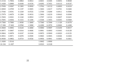
Table 1 reports the summary statistics for repo rates, in level and …rst di¤erence. All variables

are expressed in percentage points per annum. The data display similar properties to those described

by Longsta¤ (2000b) for a shorter sample. The mean of the repo rates displays a mild smile e¤ect

across the term structure. In particular, the mean overnight rate of3:9600is slightly higher than the

mean one-week rate of3:9492, which turns out to be the lowest mean across the di¤erent maturities.

The mean three-month rate is 3:9924, which is approximately3 bpshigher than the mean overnight

rate. Table 1 also reports the mean repo rates for the di¤erent maturities by day of the week and

shows a number of calendar regularities in the data. The mean repo tends to increase from Monday

to Tuesday and to decrease afterward, while the mean on Monday is always higher than the mean

on Friday. For example, the mean overnight rate on Monday is3:9718, which is about5 bpshigher

than the mean overnight rate on Friday, equal to 3:9260. A similar pattern is observed for all other

rates. However, these unconditional means are all close to one another, and the di¤erences are much

smaller than the di¤erences observed on other interest rates typically used in empirical research on

the EH. For example, compare the means of repo rates to the means of T-bill rates. In Table 2 we

report descriptive statistics on daily one-month and three-month US T-bill rates, also obtained from

Bloomberg, both for a long sample from 1961 to 2005 and for the same sample as the repo rates data.

2

The di¤erences in the unconditional means between the one-month and three-month T-bill rates over

the 1991–2005 sample are often about 15 bps, approximately …ve times larger than the maximum

di¤erence observed in repo markets for the same maturities. The di¤erences in unconditional means

for the full sample are even larger, up to 25 bps. Before embarking in our econometric analysis

designed to test the EH, it is worthwhile to note that the tiny di¤erences in the unconditional means

of repo rates at di¤erent maturities suggest that risk premia in repo markets are unlikely to be of

particular economic importance. Put another way, these descriptive statistics are clearly indicative

that the EH is more likely to hold on repo rates than T-bill rates.

[INSERT TABLE 1 AND TABLE 2 ABOUT HERE]

We also report the standard deviations of daily changes in repo rates in Table 1. The overnight

rate displays a standard deviation higher than the rates at other maturities. The standard deviation

of daily changes in the overnight rate is about 18 bps, while the standard deviations for the other

rates range from 5 to 6 bps per day. The standard deviations vary somewhat across days. The

corresponding …gures for T-bill rates, given in Table 2, indicate that changes in T-bill rates display

a substantially higher dispersion than repo rates, with a standard deviation of about 16 bps for

both one-month and three-month rates. However, the standard deviation of the raw variables

(annualized percentage returns) is not the standard deviation associated with an annual holding

period. Therefore, we also report the annualized volatility (a).3 This battery of descriptive

statistics con…rms the Longsta¤ (2000b) argument that repo rates are smaller in magnitude and less

volatile than T-bills.4

3. The expectation hypothesis

The EH of the term structure of interest rates relates a long-term n-period interest ratei(_tn) to a

short-termm-period interest ratei(_tm). In the case of pure discount bonds, the EH can be stated as

i(_tn)= 1 k

k 1 X

i=0

Et[i(tm+mi) ] +c(n;m); (1)

3_{Following Lo (2002), we compute the annualized volatility as (a) =} p_{V ar[i}

t(a)], where it(a) = Pak=01it k(d)

is the sum of the daily returns, and a= 250 is the average number of trading days. The raw data are quoted on a

360-day basis and expressed in percentage points per annum. Hence, we determine the daily return asit(d) =₃₆₀it₁₀₀

for a given raw repo rate it. We also report the product of the unconditional mean times the annualized volatility,

M ean (a), because this could be interpreted as the commonly used Black’s volatility for caps under the assumption

of log-normality.

where c(n;m) _{is the term premium between the n- and m-period bonds (and could vary with the}

maturity of the rates);k=n=m and is restricted to be an integer; andEt denotes the mathematical

expectation conditional on information set It available at timet.

In a market in which expectations are formed rationally, an investor could either invest funds

in a long-term n-period discount bond and hold it until maturity or buy and roll over a sequence

of short-term m-period discount bonds across the life of the long-term bond. Under the EH, these

strategies should di¤er only by a constant term. As result, the long-term rate should be determined

by a simple average of the current and expected future short-term rates plus a time-invariant term

premium.5 If the term premium c(n;m) is zero, the resulting form of the EH is often termed the “pure EH.”

While much of the relevant literature relies on single equation tests of the EH, derived by

repa-rameterizing Eq. (1), a number of scholars reconsider the EH in a linear VAR framework and test

the set of nonlinear restrictions that would make the VAR model consistent with the EH (Campbell

and Shiller, 1991; Bekaert and Hodrick, 2001; and Sarno, Thornton, and Valente, 2007).6 However,

while the EH postulated in Eq. (1) is only a statement about how longer-term rates are related

to expected short-term rates, the VAR setting further assumes a joint linear stochastic process for

the dynamics of the long-term and short-term interest rates. This is a convenient assumption to

extract predictions of future short-term rates by using current and past values of interest rates as

information set. The VAR model is also inspired by the a¢ ne term structure literature in which

conditional means are linear in a set of Markovian state variables (Du¢ e and Singleton, 1999; Dai

and Singleton, 2000; Jagannathan, Kaplin, and Sun, 2003; Ahn, Dittmar, and Gallant, 2002; Bansal

and Zhou, 2002; and Clarida, Sarno, Taylor, and Valente, 2006). This literature generally shows that

a¢ ne speci…cations are unable to simultaneously match conditional means and conditional variances,

leading to term premium puzzles.7 Therefore, the linear VAR framework is rooted in a literature

that has the potential to inherit some of the challenges faced by more traditional a¢ ne term structure

5_{Fama (1984) derives Eq. (1) by assuming that the expected continuously compounded yields to maturity on all}

discount bonds are equal, up to a constant, while Shiller, Campbell, and Schoenholtz (1983) show that Eq. (1) is exact in some special cases and that it can be derived as a linear approximation to a number of nonlinear expectation theories of the term structure. For coupon bonds and consols withn=₁, Shiller (1979) derives a similar linearized model in which the long-term rate is a weighted average of expected future short-term rate plus a constant liquidity premium. Finally, as shown by Longsta¤ (2000a), all traditional forms of the EH can be consistent with absence of arbitrage if markets are incomplete.

6_{The VAR methodology has been popular in the context of formulating and estimating dynamic linear rational}

expectations models since the 1970s, starting from Sargent (1977), Hansen and Sargent (1980), Sims (1980), and Wallis (1980).

7_{Another stream of the literature also shows that a¢ ne structures cannot capture what is termed “unspanned}

models. This means that one cannot rule out that the impact of these issues on EH tests based on

the VAR framework is substantial. For example, potential biases of the EH tests would arise if the

interest rates data are generated by a process that is not encompassed within the VAR framework

due to nonlinearities or time-varying covariances. In short, EH tests based on a VAR context are

valid only under the maintained hypothesis that a linear VAR accurately describes the process of

the short- and long-term interest rates and the relation between them. This maintained assumption

is questionable due to the well-documented limitations of a¢ ne speci…cations in matching the level

and term premium in bonds simultaneously with the volatility of interest rates.

These caveats notwithstanding, in this paper we rely on the VAR testing framework developed by

Bekaert and Hodrick (2001) because of its desirable power properties in presence of highly nonlinear

restrictions. Speci…cally, we implement the generalized method of moments (GMM) to estimate a

constrained VAR, which forces the data to yield the relation postulated by the EH, and then test

the validity of these restrictions by using the Lagrange multiplier (LM) and distance metric (DM)

statistics.8

3.1. The VAR framework

Consider a bivariate VAR representation for the short- and long-term interest rates measured as

deviations from their respective means:

i(_tm) = a(L)i(_tm₁)+b(L)i(_tn)₁+u1;t (2)

i(_tn) = c(L)i(_tm₁)+d(L)i(_tn)₁+u2;t; (3)

wherea(L),b(L),c(L), andd(L)are polynomials in the lag operator of orderp, andu1;tand u2;t are

error terms. For the sake of notational convenience and without loss of generality, we setc(n;m)_{= 0}

in Eq. (1) and use demeaned data in our analysis. This implies that we cannot discriminate between

the standard formulation of the EH and the pure EH with a zero average term premium, but we

focus on testing whether the term premium is constant over time.

The above formulation can be interpreted as a system in which the forecasting Eq. (2) is used

to generate the expected future short-term rate and Eq. (3) determines the current long-term

rate. Simultaneously, the system determines endogenously both sides of the EH statement given in

8_{A simple alternative would be to estimate the model without restrictions by least squares and to apply a Wald test.}

Eq. (1) and allows joint estimation of the parameters. This improves e¢ ciency by incorporating

contemporaneous cross-correlation in the errors (Pagan, 1984; and Mishkin, 1982).

The EH implies a set of nonlinear restrictions on the parameters of the above system. To de…ne

these restrictions, let us simplify the notation by translating the above p-order system into a

…rst-order VAR companion form as

2 6 6 6 6 6 6 6 6 6 6 6 6 4

i(_tm) i(_tn) i(_tm₁) i(_tn)₁

.. .

i(_{t p}m)₊₁ i(_{t p}n)₊₁

3 7 7 7 7 7 7 7 7 7 7 7 7 5 = 2 6 6 6 6 6 6 6 6 6 6 4

a1 b1 ap 1 bp 1 ap bp

c1 d1 cp 1 dp 1 cp dp

1 1 . .. 1 1 3 7 7 7 7 7 7 7 7 7 7 5 2 6 6 6 6 6 6 6 6 6 6 6 4

i(_tm₁) i(_tn)₁ i(_tm₂) i(_tn)₂

.. .

i(_{t p}m) i(_{t p}n)

3 7 7 7 7 7 7 7 7 7 7 7 5 + 2 6 6 6 6 6 6 6 4

u1;t

u2;t

3 7 7 7 7 7 7 7 5 ; (4)

where the blank elements are zeros. In compact form, this VAR can be expressed as

Yt= Yt 1+ t; (5)

where Yt has 2p elements, is a 2p square companion matrix, and vt is the vector of innovations

orthogonal to the information set available at time t, with zero mean and covariance matrix .

Then, the EH subjects Eq. (5) to the following set of nonlinear cross-equation restrictions:

e0₂ =e0₁k 1(I m) 1(I n); (6)

where e1 = (1;0; : : : ;0)0 and e2 = (0;1;0; : : : ;0)0 are 2p dimensional indicator vectors.9 Although

Eq. (6) does not have a straightforward intuition, it gives a 2p dimensional vector of restrictions,

nonlinear in the underlying parameters of , such that the predictions of future short-term rates are

consistent with the EH and the resulting constrained VAR collapses to Eq. (1). We can interpret

these restrictions as a concise summary of the main implications stated by the theory. First,

the constrained VAR de…nes the theoretical long-term rate we would observe in a world in which

expectations about future short-term rates are formed rationally. Second, under these restrictions,

the long-term rate contains all relevant information required by the market participants to predict

future short-term rates. Put another way, the long-term rate provides optimal predictions of future

short-term rates and deviations of the actual long-term rate from the theoretical long-term rate are

unsystematic and unpredictable. Then, by rewriting the 2p dimensional vector of restrictions as

a( ) =e0₂ e0₁k 1(I m) 1(I n); (7)

9_{Section A.1 in the Appendix provides further technical details on the restrictions implied by the EH in the VAR}

we can de…ne the null hypothesis of rational expectations and constant term premium as

H0:a( ) = 0; (8)

where is formed by collecting the relevant parameters of the companion matrix .10

3.2. The VAR tests

Bekaert and Hodrick (2001) propose a feasible method based on the GMM to estimate the VAR

model under the hypothesis that the EH holds, de…ned by the nonlinear cross-equation restrictions

on the parameters .11

Let yt [i(tm); i

(n)

t ] be the vector of data available at time t, ut be the vector of orthogonal

errors de…ned by the model, and xt 1 be the vector of instruments available at timet 1, formed

by stacking lagged values of yt (and possibly a constant term). Next, de…ne the vector zt

(y_t0; x0_{t 1})0, the vector-valued function of the data and the parameters g(zt; ) ut xt 1, and the

set of orthogonality conditions E[g(zt; )] 0. Using the corresponding sample moment conditions

gT( ) T 1PTt=1g(zt; )for a sample of sizeT, the parameters, , are estimated by minimizing the

GMM criterion function

QT( ) gT( )0 _T1gT( ); (9)

where _T1is a positive semide…nite weighting matrix (Hansen, 1982).12 To estimate the parameters,

, subjected to the nonlinear restrictions de…ned by Eq. (6), we de…ne the Lagrangian as

L( ; ) = 1 2gT( )

0 1

T gT( ) aT( )0 ; (10)

where is a vector of Lagrange multipliers, andaT( )is the sample counterpart ofa( ). While direct

maximization of the Lagrangian is di¢ cult as the constraints are nonlinear, Bekaert and Hodrick

(2001) develop a recursive algorithm that extends the estimator proposed by Newey and McFadden

(1994).13

If the restrictions have a signi…cant impact on parameter estimation, then the value of the

La-grange multipliers is signi…cantly di¤erent from zero and the null hypothesis that the EH holds is

1 0

Speci…cally, the vector of parameters is de…ned as = (a1; ; ap; b1; ; bp; c1; ; cp; d1; ; dp)0.

1 1

Full maximum likelihood estimation of the restricted model is generally considered as cumbersome (e.g., Bekaert and Hodrick, 2001; and Melino, 2001).

1 2

When T is chosen optimally,bis asymptotically distributed as

p

T(b 0)!N(0; G0T TGT) 1, where 0denotes the true parameters,bthe parameter estimates,GT rgT( )the gradient of the orthogonality conditions, and the

symbol_!convergence in distribution.

1 3_{The GMM estimation is applied to the VAR de…ned in Eqs. (2) and (3), whereas the companion VAR is exclusively}

rejected. The hypothesis that the multipliers are jointly zero can be tested using the LM statistic

T ATB_T1A0T ! 2(2p) (11)

or the DM statistic

T gT( )0 T1gT( ) ! 2(2p); (12)

where denotes the constrained estimates, and2p is the number of restrictions implied by the EH.

3.3. Small sample properties

Tests of the EH null hypothesis have been known to su¤er severely from problems related to

…nite sample bias estimation errors. In essence, the sampling distribution in …nite sample could be

signi…cantly di¤erent from the asymptotic distribution (e.g., Bekaert, Hodrick, and Marshall, 1997;

Bekaert and Hodrick, 2001; and Thornton, 2005, 2006). Thus, before estimating the unconstrained

and constrained VARs, we follow Bekaert and Hodrick (2001) and use two di¤erent data generating

processes (DGPs). Speci…cally, from the original data set, we simulate via bootstrap two

bias-corrected data sets of 70 thousand observations, with homoskedastic innovations and generalized

autoregressive conditional heteroskedasticity (GARCH) innovations, and we use them throughout

the econometric analysis. See Section A.3 in the Appendix for technical details on the procedure to

account for small-sample bias in our analysis.

4. Empirical results I: the VAR test of the EH

In the empirical analysis, we obtain the unconstrained parameter estimate of , denoted b, by

least squares and its constrained estimate by the constrained GMM scheme for all possible pairwise

combinations of short- and long-term rates such that k=n=m is an integer. To take into account

the day-of-the-week regularities in the short-term repo rates, shown in Table 1, we follow Longsta¤

(2000b) and set the VAR lag length to bep= 5.

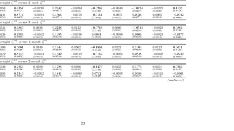
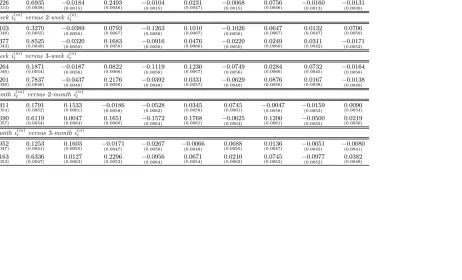
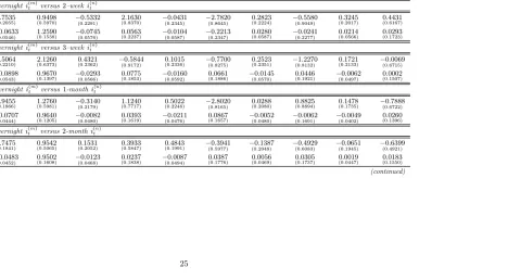
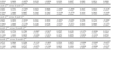
Tables 3 and 4 report bias-corrected coe¢ cients for the unconstrained VARs and the constrained

VARs that satisfy the EH, respectively, when the DGP used to bias correct the parameters assumes

homoskedastic innovations. Comparing the coe¢ cients in Tables 3 and 4, we note that sharp

di¤erences exist in the constrained and unconstrained estimated dynamics. In particular, for each

pairwise comparison, we …nd that the standard errors are large in the constrained VAR. Also, the

absolute size of the constrained coe¢ cients is much larger than the corresponding unconstrained ones,

and, perhaps more important, the constrained coe¢ cients measuring the response of the short-term

estimates. This is prima facie evidence that the EH restrictions could be inconsistent with the data,

although this evidence does not constitute a formal statistical test.

[INSERT TABLE 3 AND TABLE 4 ABOUT HERE]

For robustness, we also carry out estimation of the VAR-GARCH model.14 We …nd that the

factor loadings are statistically signi…cant at standard signi…cance levels, indicating the presence of

GARCH e¤ects. We also notice that the conditional variance turns out to be persistent for the

overnight repo and moderately persistent for the spreads. Hence, departing from the assumption of

homoskedasticity is likely to yield more accurate estimates of the VAR parameters and, consequently,

more precise tests of the EH.

We then estimate the bias-corrected coe¢ cients for the unconstrained VARs and the constrained

VARs that satisfy the EH, respectively, when the DGP used to bias correct the parameters assumes

GARCH innovations. These results are quantitatively di¤erent from but qualitatively identical to

the results for the VAR with homoskedastic innovations given in Tables 3 and 4. Speci…cally, the

standard errors of parameters estimates in the constrained VAR are large, the absolute size of the

constrained coe¢ cients is larger than the corresponding unconstrained ones, and the constrained

coe¢ cients measuring the response of the short-term rate to the long-term rate have sometimes a

di¤erent sign from the corresponding estimates in the unconstrained VAR.

4.1. LM and DM tests of the EH

The LM and DM tests results are presented in Table 5, where we report the p-values for the

null hypothesis that the EH holds for all possible repo rates combinations of the integer k =n=m.

The results in Table 5 indicate that the EH is rejected for each rate pair with p-values that are

well below standard signi…cance levels. Table 5 also reports the p-values from the J-test, which

provides a speci…cation test of the validity of the overidentifying moment conditions. The p-values

are comfortably larger than conventional signi…cance levels, validating the GMM estimation and,

hence, the LM and DM tests.

[INSERT TABLE 5 ABOUT HERE]

1 4

These …ndings di¤er from Longsta¤ (2000b), who does not reject the EH using conventional

tests, because the VAR test is particularly powerful (and, thus, more likely to detect …ne departures

from the null hypothesis in …nite sample) and because our sample is larger than that in Longsta¤

(2000b). However, despite this statistical evidence, a legitimate and unanswered concern is whether

the rejection of the EH could be due to small departures from the null hypothesis (or tiny data

imperfections) that are not economically meaningful but appear statistically signi…cant given the

powerful test statistics and the very large sample size employed.15 Moreover, the VAR tests are not

designed to incorporate the fact that if one wanted to trade on departures from the EH, instead of

assuming that the EH holds in a simple buy-and-hold allocation strategy, transactions costs create

a wedge between returns from an active strategy exploiting departures from the EH and a simple

buy-and-hold strategy. Finally, while the VAR tests rely on the ability of the VAR to capture

the time-series properties of the term structure of repo rates, we are aware that the simple VAR

tests, inspired by the literature on a¢ ne term structure models, is unable to satisfactorily explain

conditional means and volatility of interest rates. Hence, potential model misspeci…cation and model

uncertainty could play an important role in determining the rejection of the EH recorded in Table

5. To address these issues and to shed light on the economic signi…cance of the statistical rejections

of the EH recorded in this section, we proceed to an economic evaluation of the EH departures.

5. Measuring the economic value of deviations from the EH

We wish to measure whether departures from the EH provide information that is economically

valuable, regardless of whether or not they are statistically signi…cant on the basis of econometric

tests. This section discusses the framework we use to evaluate the impact of allowing for deviations

from the EH on the performance of dynamic allocation strategies in the repo market. We employ

mean-variance analysis as a standard measure of portfolio performance assuming quadratic utility.

Ultimately, we aim at measuring how much an investor is willing to pay for switching from a strategy

that assumes that the EH holds (_EHstrategy) to a dynamic strategy that conditions on departures

from the EH (_DEH strategy). The _EH strategy uses the outcome from the constrained VAR to

determine the portfolio allocation, whereas the _DEH strategy is based on the unconstrained VAR.

The allocation strategy we consider is simple and intuitive. It consists of taking a position (either

long or short) in a long-term repo, and then hedging it with an o¤setting rolling position in a series of

1 5

short-maturity repos. If the EH governs the relation between the long-term and short-term rates and

an investor takes long positions in long-term repos and short rolling positions in short-term repos,

then following this strategy over time allows the investor to earn the unconditional term premium,

denoted as c(n;m) in Eq. (1). However, if one thinks of all repo rates in deviations from their

unconditional mean (i.e., settingc(n;m)= 0), as we do in our setting below, then this strategy should

earn a return of zero before costs.

Regardless of the EH rejections recorded in Table 5, the tiny di¤erences in unconditional means

of repo rates at di¤erent maturities observed in Table 1 suggest the possibility that the economic

value of trading on deviations from the EH in the repo market might not be as appealing as the

statistical rejections from the VAR tests could imply. The investor using the constrained VAR is

e¤ectively using the simple strategy described above based upon the belief no di¤erences exist in

the returns from investing in the longer repo rate and from investing in a series of shorter repo

rates. However, if the investor does not believe in the EH and hence uses the unconstrained VAR,

the resulting allocation strategy is the outcome of the predictions of the model with respect to

whether the longer-term rate is under or overvalued relative to the series of shorter repo rates over

the maturity of the longer rate. This could be seen as the implementation of the popular carry

trade strategy that attempts to exploit mispricing along the term structure of interest rates. In

other words, using the unconstrained VAR is tantamount to exploiting the deviations from the EH,

which we have recorded in the earlier statistical analysis. If the unconstrained VAR model gives

predictions of short-term repo rates consistent with the EH, the results from the_EHstrategy should

be equal to the results from the _DEH strategy.16 From this setting we can calculate directly a

variety of common performance measures, in the form of performance fees _F (Fleming, Kirby, and

Ostdiek, 2001) and risk-adjusted abnormal returns_M(Modigliani and Modigliani, 1997).

We realize that a portfolio consisting only of repo rates is unlikely to be a realistic portfolio

managed by a US investor. The repurchase agreements involving US Treasury securities are mainly

used by banks to manage the quantity of reserves on a short-term basis and, hence, play an important

role in the Federal Reserve’s implementation of monetary policy. Moreover, the repo market plays a

fundamental role in dealers’hedging activities, and repos are used by investment managers who sell

short Treasury securities to hedge the interest rate risk in other securities. Our main objective is not

to design a realistic (executable) asset allocation strategy, but to measure the economic signi…cance

of deviations from the EH. Our measures of economic value complement the LM and DM tests

1 6

for statistical signi…cance of the EH by showing whether the constraints imposed on the VAR by

the EH have economic value. On the one hand, departures from the EH could be statistically

insigni…cant and yet provide considerable value to an investor. On the other hand, the departures

might be statistically signi…cant but be of little or no economic value to a repo market investor.17

This economic evaluation is easier to carry out and assess by focusing exclusively on a VAR in which

the only assets being modeled are repo rates at various maturities, because the only source of risk

in the resulting repo portfolio is interest rate risk.

5.1. The EH in a dynamic mean-variance framework

In mean-variance analysis, the maximum expected return strategy leads to a portfolio allocation

on the e¢ cient frontier. Speci…cally, consider the trading strategy of an investor who has ak-period

horizon and constructs a daily dynamically rebalanced portfolio that maximizes the conditional

expected return subject to achieving a target conditional volatility. Computing the time-varying

weights of this portfolio requires predictions of the k-period ahead forecast of the conditional mean

and the conditional variance-covariance matrix.

Let rt+k denote the N 1 vector of risky asset returns; t+kjt = Et[rt+k] is the conditional

expectation of rt+k; and t+kjt = Et[(rt+k t+kjt)(rt+k t+kjt)0] is the conditional

variance-covariance matrix ofrt+k.18 At each period t, the investor solves the following problem:

max

wt f p;t+k

=w_{t t}0 _+kjt+ 1 w_t0 rfg (13)

s.t. _p 2=w_t0 t+kjtwt;

wherewtis theN 1vector of portfolio weights on the risky assets, p;t+kis the conditional expected

return of the portfolio, _p is the target conditional volatility of the portfolio returns, and rf is the

return on the riskless asset.19 The solution to this optimization problem delivers the following risky

asset weights:

wt= pp

Ct

1

t+kjt( t+kjt rf); (14)

whereCt= ( t+kjt rf)0 _t+1_kjt( t+kjt rf). The weight on the riskless asset is1 wt0 .

By design, in this setting the optimal weights vary across models only to the extent that

predic-tions of the conditional moments vary, which is precisely what the empirical models provide. In our

1 7_{See Leitch and Tanner (1991) for an early treatment of the relation between statistical signi…cance and economic}

value.

1 8

We use the subscriptt+kto indicate an investment horizon ofkperiods ahead, wherek=n=mis an integer that depends on the long- and short-term interest rates.

1 9_{For simplicity, we drop the subscripttfrom the riskless returnr}

setting, we carry out the economic value analysis comparing the outcome from the_DEHstrategy (a

strategy that exploits deviations from the EH) with the _EH strategy, which assumes that the EH

holds. We compute the calculations for both cases with homoskedastic and GARCH innovations in

the bias-correction DGPs. In short, our objective is to determine whether there is economic value

in using the unconstrained VAR, which relaxes the constraints imposed by the EH.

5.2. Quadratic utility

We rank the performance of the competing repo rate models using the West, Edison, and Cho

(1993) methodology, which is based on mean-variance analysis with quadratic utility. The investor’s

realized utility in periodt+k can be written as

U(Wt+k) =Wt+k

2W

2

t+k=WtRp;t+k

W_t2

2 R

2

p;t+k; (15)

whereWt+k is the investor’s wealth at t+k, determines his risk preference, and

Rp;t+k= 1 +rp;t+k= 1 + 1 wt01 rf +wt0rt+k (16)

is the period t+k gross return on his portfolio.

We quantify the economic value of deviations from the EH by setting the investor’s degree of

relative risk aversion (RRA), t = Wt=(1 Wt), equal to a constant value . In this case,

West, Edison, and Cho (1993) demonstrate that one can use the average realized utility, U( ), to

consistently estimate the expected utility generated by a given level of initial wealth. Speci…cally,

the average utility for an investor with initial wealth W0 is equal to

U( ) =W0

T_X1

t=0

Rp;t+k

2 (1 + )R

2

p;t+k : (17)

We standardize the investor problem by assuming the investor allocates $1 in every time period.

Average utility depends on taste for risk. In the absence of restrictions on , quadratic utility

exhibits increasing degree of RRA. This is counterintuitive because, for instance, an investor with

increasing RRA becomes more averse to a percentage loss in wealth when his wealth increases. As in

West, Edison, and Cho (1993) and Fleming, Kirby, and Ostdiek (2001), …xing the degree of RRA, ,

implies that expected utility is linearly homogeneous in wealth: double wealth and expected utility

doubles. Furthermore, by …xing instead of , we are implicitly interpreting quadratic utility as

an approximation to a nonquadratic utility function, with the approximating choice of dependent

Fleming, Kirby, and Ostdiek (2001) framework for assessing the economic value of the_DEH and_EH

strategies.20

5.3. Performance measures

At any time, one set of estimates of the conditional moments is better than a second set if

invest-ment decisions based on the …rst set lead to higher average realized utility,U. Alternatively, a better

model requires less wealth to yield a given level ofU than the alternative model. Following Fleming,

Kirby, and Ostdiek (2001), we measure the economic value of the interest rate strategies by equating

the average utilities for selected pairs of portfolios. Suppose, for example, that holding a portfolio

constructed using the optimal weights based on the _EH strategy yields the same average utility as

holding the portfolio implied by the_DEH strategy. The latter portfolio is subject to daily

manage-ment expenses _F, expressed as a fraction of wealth invested in the portfolio. Because the investor

would be indi¤erent between these two strategies, we interpret_F as the maximum performance fee

the investor would be willing to pay to switch from the _EH to the _DEH strategy. In general, this

utility-based criterion measures how much an investor with a mean-variance utility function is

will-ing to pay for conditionwill-ing on the deviations from the EH, as presented in the unconstrained VAR

model.21

The performance fee depends on the investor’s degree of risk aversion and is a measure of the

economic signi…cance of violations of the EH. To estimate the fee, we …nd the value of _F that

satis…es

T_X1

t=0

RDEH_{p;t+k F}

2 (1 + ) R

DEH

p;t+k F

2

=

T_X1

t=0

REH_p;t+k

2 (1 + ) R

EH

p;t+k

2

; (18)

where RDEH_p;t+k denotes the gross portfolio return constructed using the predictions from the

uncon-strained VAR model, andR_p;tEH_+kis the gross portfolio return implied by the constrained VAR model. In the absence of transactions costs, under the EH, _F = 0, while, if the EH is violated, _F > 0.

However, when allowing for transactions costs, it is also possible that_F <0if the positive gain from

2 0

A critical aspect of mean-variance analysis is that it applies exactly only when the return distribution is normal or the utility function is quadratic. Hence, the use of quadratic utility is not necessary to justify mean-variance optimization. For instance, one could instead consider using utility functions belonging to the constant relative risk aversion (CRRA) class, such as power or log utility. However, quadratic utility is an attractive assumption because it provides a high degree of analytical tractability. Quadratic utility could also be viewed as a second-order Taylor series approximation to expected utility. In an investigation of the empirical robustness of the quadratic approximation, Hlawitschka (1994) …nds that a two-moment Taylor series expansion “may provide an excellent approximation” (p. 713) to expected utility and concludes that the ranking of common stock portfolios based on two-moment Taylor series is “almost exactly the same” (p. 714) as the ranking based on a wide range of utility functions.

2 1_{For studies following this approach, see also Fleming, Kirby, and Ostdiek (2003), Marquering and Verbeek (2004),}

trading on the information provided by the EH violation is lower than the loss incurred by the more

costly dynamic rebalancing of the _DEH strategy.

We also consider the Modigliani and Modigliani (1997) measure _M, which de…nes the abnormal

return that the_DEH strategy would have earned over the_EHstrategy if it had the same risk as the

EH strategy

M= [_{EH](_SRDEH _SREH); (19)

where_SR=E[_{]= [_{]is the Sharpe Ratio, andE[_{]and [_{]are the expected value and standard

deviations of the excess return,_{, of a selected strategy, respectively. The_DEHstrategy is leveraged

downward or upward, so that it has the same volatility as the _EH strategy. Therefore, the

risk-adjusted abnormal return, _M, measures the outperformance of the _DEH strategy with respect to

the_EH strategy while matching the same level of risk.22

5.4. Dynamic strategies, transaction costs and short selling

Consider a US investor who allocates his wealth between a long–term n-period discount bond

and a sequence of kshort-term m-period discount bonds. The long-term bond price is known with

certainty and implies a riskless return, whereas the rolling combination of short-term bonds generates

a risky return, because k 1 future short-term bond prices are not known. Hence, on the basis of

riskless return,rf, and the forecasts of the conditional moments of risky return,rt+kjt, the investor

de…nes his portfolio optimization problem at timet.

We consider two alternative trading strategies. The_EHstrategy assumes that EH holds exactly,

and hence the investor takes a position using forecasts based on the constrained VAR. In this case,

the investor e¤ectively trades assuming that Eq. (1) holds and, in the absence of transactions costs,

he is indi¤erent between investing in the long rate or a series of short rates. However, if transactions

costs are positive and equal for short- and long-rates, the investor prefers investing in the long

rate as this minimizes costs. The _DEH strategy uses the forecasts based on the unconstrained

VAR. Speci…cally, each strategy is made up of two steps at time t. First, the investor uses the

selected VAR model to generate the conditional moments of the rolling strategy, _t+kjt and _t+kjt.

Second, conditional on the predictions of this model and given the riskless returnrf, he dynamically

rebalances his portfolio by computing optimal weights. He repeats this process every day until the

end of the sample period.23

2 2

We also compute a measure that allows for downside risk. However, because the results are qualitatively identical to the performance fees and risk-adjusted abnormal returns, we do not report them here to conserve space.

2 3_{Because we consider a single risky return,}

This setup determines whether using one particular conditional speci…cation a¤ects the

perfor-mance of a short-horizon allocation strategy in an economically meaningful way. The predictions

are all in-sample predictions, because our focus is not to provide forecasting models of the repo term

structure but to evaluate the measured departures from the EH as determined by the unconstrained

VAR model.

With daily rebalancing, transaction costs play an important role in evaluating the relative

per-formance of di¤erent strategies. In particular, we assume that transaction costs at time t equal a

…xed proportion of the value traded in long-term and short-term repos (Marquering and Verbeek,

2004; and Han, 2006). We also assume that the costs are the same for trading short and long rates.

This is consistent with the fact that the bid-ask spread is fairly constant across maturities in the

repo market, in the order of 2 to 5 bps. We report results both with and without transactions

costs and also study the impact of short selling constraints. In the case of limited short selling we

constrain the portfolio weights to be bounded between 1 and 2 (assuming that the investor can

borrow no more than 100% of his wealth), while in the case of no short selling, the portfolio weights

are constrained between 0 and1.

6. Empirical results II: the economic value of EH departures

Given the VAR parameter estimates described above, we assume that a US investor dynamically

updates his portfolio weights daily after reestimating the VAR model with the latest available data.

The key question is whether the dynamic strategy that allows for departures from the EH generates

economic gains relative to a benchmark dynamic strategy that assumes that the EH holds. We

assess the economic value of conditioning on departures from the EH by analyzing the performance

of the dynamically rebalanced portfolio constructed using pairwise combinations of repo rates.24

We compute the performance fee _F and the risk-adjusted abnormal return _Mfor (1) two target

annualized portfolio volatilities, _p = _f1%;2%_g, which are in a range that includes the observed

annualized standard deviation of the data reported in Table 1; (2) a degree of relative risk aversion

= 5; (3) for each pair of repo maturities where the long maturity is an exact multiple of the

short maturity; and (4) two di¤erent DGPs for the parameter estimates, with homoskedastic and

heteroskedastic innovations.25 Furthermore, we also exploit the impact of transaction costs and

short selling by considering four di¤erent scenarios. In Case 1 transaction costs are ignored and the

weights are unrestricted; in Case 2 the weights are unrestricted but we introduce transaction costs

with = 4 bps, a realistic cost on the basis of the observed bid-ask spread in the repo market; in

2 4_{For weekends and holidays we consider the rate on the previous business day for which a rate was reported.} 2 5

Case 3 we also add a limited short selling constraint by restricting the weights to be between 1

and 2; and in Case 4 we do not allow short selling so that the weights are between0 and 1. The

performance measures,_F and _M, are reported in annualized basis points.26

6.1. Performance measures

Table 6 presents the in-sample performance fees _F and the risk-adjusted abnormal returns _M

for the _DEH strategy against the _EH strategy when the bootstrap experiment for bias correction

assumes homoskedastic innovations. Panel A reports the results for a target volatility _p = 1%, and

Panel B for _p = 2%.

[INSERT TABLE 6 ABOUT HERE]

The results in Table 6 suggest that the performance fees for switching from a model that assumes

the EH holds to a model that exploits departures from the EH is generally fairly modest when we

do not consider transaction costs and the portfolio weights are unrestricted (Case 1). For example,

if we set the target volatility at _p = 1%, the annual performance fee a risk-averse investor would

be willing to pay to switch from the _EH strategy to the _DEH strategy is at most 1:34 bps. If we

calibrate the target volatility to be _p = 2%, the largest annual performance fee reaches 2:70 bps

and occurs when the overnight repo rate is the short-term rate and the one-week repo rate is the

long-term rate.

However, when we introduce transaction costs (Case 2), the performance fees _F become even

smaller and are slightly negative at the shorter end of the maturity spectrum. For instance, given

p = 1%and the overnight repo rate versus the three-week repo rate, theDEHstrategy has a negative

annual performance fee of about3bps. This suggests that the higher transactions costs incurred in

the _DEH strategy outweigh the bene…t of conditioning on EH violations, with the performance fee

generally decreasing in k =m=n due to the larger number of trades needed in the rolling strategy.

In other words, the EH violations are not economically signi…cant after costs are taken into account.

When we move at the longer spectrum of the maturity and consider one-month versus three-month

repo rates for _p = 1%, we notice a performance fee of 0:49 bps. When we combine transaction

costs and limited short-selling (Case 3), the performance measures remain virtually the same as

in Case 2, suggesting that the weights are in the range from 1 and 2. In the fourth scenario,

2 6

we consider dynamic strategies without short selling and with transaction costs (Case 4). In this

case the fees decrease moderately in absolute values con…rming that the short selling constraints are

now binding on the pro…tability of the strategies, but their impact is modest. The risk-adjusted

abnormal returns_Mare of similar magnitude as (in some columns identical to) the performance fees

F, leading therefore to the same conclusions.

For robustness purposes, Table 7 reports the same performance criteria, _F and _M, when we

assume GARCH innovations for the bias correction procedure. The results are qualitatively identical

to the case of the VAR with homoskedastic errors discussed in Table 6, providing evidence that EH

violations are economically unimportant. However, quantitatively the results in Table 7 provide

evidence of even smaller gains from the _DEHstrategy, with the performance fee _F never reaching 2

bps.

[INSERT TABLE 7 ABOUT HERE]

7. Conclusions

The EH plays an important role in economics and …nance and, not surprisingly, has been widely

tested using a variety of tests and data. Much of the empirical literature has struggled to …nd

evidence supporting the validity of the EH across a variety of data sets and countries and employing

increasingly sophisticated testing procedures. This paper reexamines an important exception in

this literature: the result that the EH appears to …t the behavior of US repo rates at the shortest

end of the term structure, measured at daily frequency from overnight to the three-month maturity

(Longsta¤, 2000b). We innovate in this context on two grounds. First, we extend this research by

testing the restrictions implied by the EH on a VAR of the long- and short-term repo rate using the

test proposed by Bekaert and Hodrick (2001). These results are not encouraging for the EH, which

is statistically rejected across the term structure considered.

Second, we move beyond statistical tests and provide complementary evidence on the validity

of the EH using some economic value calculations. We assess the economic value of exploiting

departures from the EH (i.e., using empirical models that condition on information contained in

EH deviations) relative to the economic value of using a model that assumes the EH holds. The

empirical results indicate that the economic value of departures from the EH is modest and generally

smaller than the costs that an investor would incur to exploit the mispricing implied by EH violations.

The results from economic value calculations are in contrast with the results from VAR tests

reported earlier. This di¤erence con…rms that statistical rejections of a hypothesis do not always

imply economic rejections and raises doubts about the ability of the simple linear VAR framework

to capture the relationship between repo rates at di¤erent maturities. Activities in the repo market

at maturities of days or weeks are largely driven by liquidity considerations and by the attempts of

banks to manage the quantity of reserves and to hedge interest rate risk on a short-term basis, not

to speculate in search of excess returns. Hence, it seems unlikely that investors would be actively

exploiting EH departures on a short-term basis. Our main conclusion is that, even though the EH

could be rejected statistically, it still provides a reasonable approximation to the term structure of

[image:23.595.96.760.211.514.2]

Table 1

Descriptive statistics for daily repo rates

The table summarizes the descriptive statistics for the daily repo rates (Panel A) and daily changes in repo rates (Panel B), from overnight to three-month maturity. The data set consists of 3,625 daily observations of the indicated term government general collateral repo rates from May 21, 1991 to December 9, 2005, quoted on a360-day basis and expressed in percentage points per annum. The period September 10, 2001 to September 30, 2001 is not included. The daily change in repo rate for the indicated weekday is measured from the indicated day to the next business day. ρ_idenotes thei-th order serial correlation coefficient.

σ(a) =sV ar[i_t(a)] is the annualized volatility, whereit(a) =Sa_k−₌₀1it−k(d) is the sum of the daily returns,a= 250 is the average number of trading days, and

it(d) =₃₆₀it

×100 is the daily return for a given raw repo rateit. All statistics are measured in percentage points per annum.

Panel A. Percent values Panel B. Percent daily changes

it i(1t w) i

(2w)

t i

(3w)

t i

(1m)

t i

(2m)

t i

(3m)

t ∆it ∆i(1t w) ∆i

(2w)

t ∆i

(3w)

t ∆i

(1m)

t ∆i

(2m)

t ∆i

(3m)

t

M ean 3.9600 3.9492 3.9521 3.9544 3.9623 3.9752 3.9924 −0.0004 −0.0005 −0.0005 −0.0005 −0.0005 −0.0005 −0.0004

M eanM on 3.9718 3.9433 3.9420 3.9428 3.9483 3.9599 3.9764 −0.0360 −0.0106 −0.0057 −0.0051 −0.0016 −0.0004 0.0000

M eanT ue 3.9728 3.9628 3.9657 3.9672 3.9757 3.9890 4.0051 −0.0040 −0.0064 −0.0037 −0.0029 −0.0036 −0.0035 −0.0030

M eanW ed 3.9616 3.9496 3.9544 3.9571 3.9650 3.9784 3.9952 0.0036 −0.0022 −0.0049 −0.0039 −0.0037 −0.0022 0.0002

M eanT hu 3.9683 3.9492 3.9526 3.9563 3.9642 3.9780 3.9969 −0.0330 −0.0028 −0.0006 −0.0010 0.0004 −0.0016 −0.0027

M eanF ri 3.9260 3.9403 3.9445 3.9474 3.9565 3.9692 3.9866 0.0643 0.0191 0.0123 0.0103 0.0060 0.0055 0.0033

Std Dev 1.6998 1.6944 1.6973 1.6990 1.7003 1.7007 1.7013 0.1738 0.0648 0.0524 0.0517 0.0488 0.0507 0.0567

Std DevM on 1.7039 1.7008 1.7017 1.7032 1.7023 1.7019 1.7010 0.1533 0.0672 0.0584 0.0621 0.0550 0.0517 0.0656

Std DevT ue 1.6951 1.6927 1.6959 1.6978 1.6999 1.6997 1.7009 0.1818 0.0640 0.0486 0.0498 0.0516 0.0540 0.0609

Std DevW ed 1.7115 1.7015 1.7054 1.7069 1.7072 1.7075 1.7074 0.2081 0.0621 0.0484 0.0448 0.0466 0.0484 0.0492

Std DevT hu 1.6975 1.6884 1.6927 1.6948 1.6978 1.6993 1.7009 0.1383 0.0447 0.0447 0.0463 0.0471 0.0518 0.0570

Std DevF ri 1.6953 1.6935 1.6956 1.6969 1.6991 1.6996 1.7006 0.1580 0.0779 0.0590 0.0535 0.0426 0.0470 0.0500

M in 0.8400 0.8900 0.8800 0.8700 0.8600 0.8300 0.8300 −1.5500 −0.8200 −0.8300 −0.8400 −0.8600 −0.8100 −0.8600

M ax 6.7500 6.7000 6.5000 6.4900 6.4700 6.5000 6.5800 3.4000 1.1000 0.4100 0.6300 0.2900 0.3700 0.6200

ρ1 0.9948 0.9993 0.9995 0.9995 0.9996 0.9996 0.9994 −0.3226 −0.0308 −0.1077 −0.1885 −0.1806 −0.2354 −0.2882

ρ₂ 0.9929 0.9986 0.9991 0.9992 0.9993 0.9993 0.9992 −0.0921 −0.0150 0.0420 0.0399 0.0209 −0.0158 0.0467

ρ₃ 0.9920 0.9979 0.9987 0.9989 0.9990 0.9991 0.9989 −0.0287 −0.0650 −0.0112 −0.0200 −0.0449 0.0123 −0.0345

ρ₄ 0.9914 0.9973 0.9983 0.9986 0.9988 0.9989 0.9987 −0.0041 −0.1112 0.0101 0.0388 0.0491 0.0500 0.0494

ρ5 0.9909 0.9969 0.9979 0.9983 0.9985 0.9986 0.9984 −0.0350 −0.0270 −0.0022 −0.0097 0.0276 −0.0225 0.0019

σ(a) 1.1640 1.1625 1.1654 1.1669 1.1681 1.1687 1.1691

[image:24.595.203.637.202.503.2]

Table 2

Descriptive statistics for daily Treasury bill rates

The table summarizes the descriptive statistics for daily T-bill rates,T bt, and daily changes in T-bill rates,∆T bt, for the one-month(1m)and three-month (3m)maturity, respectively. The data are measured in percentage points per annum. Panel A reports the statistics for the period June 14, 1961 to December 30, 2005 and consists of 11,110 daily observations. Panel B reports the statistics for the period May 21, 1991 to December 9, 2005 and consists of 3,568 daily observations. The daily change in the T-bill rate for the indicated maturity is measured from the indicated day to the next business day. ρ_idenotes thei-th order serial correlation coefficient. σ(a) =sV ar[i_t(a)]is the annualized volatility, where it(a) =Sa_k−₌₀1it−k(d)is the sum of the daily returns,a= 250is the average

number of trading days, andit(d) = ₃₆₀it

×100 is the daily return for a given raw repo rateit. All statistics are measured in percentage points per annum. Panel A. 1961—2005 Panel B. 1991—2005

T b(1t m) T b

(3m)

t ∆T b

(1m)

t ∆T b

(3m)

t T b

(1m)

t T b

(3m)

t ∆T b

(1m)

t ∆T b

(3m)

t

M ean 5.5130 5.7597 0.0002 0.0001 3.6823 3.8358 −0.0005 −0.0006

M eanM on 5.5339 5.7754 0.0004 0.0018 3.7016 3.8508 −0.0034 −0.0057

M eanT ue 5.5337 5.7798 −0.0044 −0.0103 3.7046 3.8584 −0.0057 −0.0102

M eanW ed 5.5424 5.7864 −0.0176 −0.0079 3.6982 3.8483 −0.0111 −0.0048

M eanT hu 5.5152 5.7694 0.0063 0.0012 3.6831 3.8405 0.0055 0.0029

M eanF ri 5.4428 5.6900 0.0160 0.0158 3.6285 3.7851 0.0113 0.0137

Std Dev 2.7856 2.8567 0.1305 0.0933 1.5764 1.6112 0.0693 0.0416

Std DevM on 2.8002 2.8709 0.1197 0.0805 1.5863 1.6217 0.0761 0.0466

Std DevT ue 2.7946 2.8591 0.1249 0.0725 1.5769 1.6200 0.0811 0.0386

Std DevW ed 2.7979 2.8678 0.1206 0.0818 1.5904 1.6219 0.0643 0.0386

Std DevT hu 2.7693 2.8501 0.1248 0.0953 1.5797 1.6124 0.0627 0.0431

Std DevF ri 2.7685 2.8382 0.1555 0.1238 1.5536 1.5855 0.0585 0.0369

M in 0.7360 0.7900 −1.8830 −1.3080 0.7360 0.7900 −1.1120 −0.8570

M ax 17.926 17.682 2.0760 1.5090 6.4290 6.2970 0.9880 0.4490

ρ₁ 0.9989 0.9995 0.0449 0.2000 0.9990 0.9997 −0.0239 0.0917

ρ₂ 0.9977 0.9987 0.0344 0.0606 0.9981 0.9993 −0.0485 −0.0130

ρ3 0.9964 0.9979 0.0187 0.0180 0.9973 0.9989 −0.0023 −0.0125

ρ₄ 0.9951 0.9971 0.0270 0.0598 0.9965 0.9985 0.0026 0.0492

ρ₅ 0.9938 0.9962 0.0718 0.0556 0.9956 0.9981 0.0305 0.0361

σ(a) 1.8488 1.9144 1.0682 1.0988

[image:25.595.133.710.163.450.2]

Table 3

Unconstrained vector autoregression (VAR) dynamics with homoskedastic innovations

The table presents the unconstrained VAR parameter estimates adjusted for small-sample bias. The data generating process used for the bias-correction assumes homoskedastic innovations. i(tn) is the n-period (long-term) rate andi

(m)

t is the m-period (short-term) rate. Each panel reports different combinations

of short-term and long-term repo rates such that k=n/mis an integer. Standard errors are reported in parenthesis.

Panel A. Overnight i(tm) versus 1—week i

(n)

t

i(tm−1) i (n)

t−1 i

(m)

t−2 i

(n)

t−2 i

(m)

t−3 i

(n)

t−3 i

(m)

t−4 i

(n)

t−4 i

(m)

t−5 i

(n)

t−5

i(tm) 0.2662

(0.0040) (00..70150086) −(00..0041)0455 0

.0347

(0.0115) −(00..0041)0146 0

.0423

(0.0115) −(00..0041)0093 −0

.0219

(0.0115) −0

.0087

(0.0040) 0

.0548

(0.0087)

i(_tn) 0.0462

(0.0018) 0

.9267

(0.0040) −0

.0238

(0.0019)

0.0305

(0.0053) −0

.0034

(0.0019) −

0.0438

(0.0053) −

0.0128

(0.0019) −

0.0427

(0.0053)

0.0008

(0.0018) 0

.1219

(0.0040)

Panel B. Overnight i(_tm) versus 2—week i(_tn)

i(_tm) 0.3258

(0.0039) 0

.4357

(0.0104) −0

.0210

(0.0041)

0.2842

(0.0137) −0

.0094

(0.0041) −

0.0262

(0.0138) −

0.0048

(0.0041) −

0.0774

(0.0137) −

0.0223

(0.0039)

0.1135

(0.0106)

i(tn) 0.0241

(0.0014) (00..87140039) −(00..0015)0194 0

.1566

(0.0051) −(00..0015)0176 −0

.0164

(0.0051) −0

.0071

(0.0015) 0

.0026

(0.0051) (00..00950014) −(00..0040)0042 Panel C. Overnight i(_tm) versus 3—week i(_tn)

i(_tm) 0.3544

(0.0039) (00..38890108) (00..00360041) (00..27380137) (00..01220041) −(00..0139)0763

0.0060

(0.0041) −(00..0138)0514 −

0.0023

(0.0038)

0.0884

(0.0111)

i(tn) 0.0126

(0.0014) (00..79840039) −(00..0015)0162 0

.1985

(0.0049) −(00..0015)0190 0

.0083

(0.0050) −(00..0015)0096 0

.0466

(0.0049) −(00..0014)0024 −0

.0177

(0.0040)

Panel D. Overnight i(tm) versus 1-monthi

(n)

t

i(tm) 0.4106

(0.0038) (00..30610116) (00..03460041) (00..19440149) (00..03620041) −(00..0150)1804 0

.0221

(0.0041) 0(0..10040149) (00..01230038) (00..06110119)

i(_tn) 0.0179

(0.0013) (00..81460038) −(00..0014)0164

0.1630

(0.0049) −(00..0014)0118 −

0.0162

(0.0049) −

0.0085

(0.0013)

0.0848

(0.0049) −(00..0012)0038 −

0.0240

(0.0039)

Panel E. Overnight i(_tm) versus 2-monthi(_tn)

i(_tm) 0.4539

(0.0038) 0

.2259

(0.0116) 0

.0589

(0.0042) 0

.1228

(0.0143) 0

.0596

(0.0042) −0

.1476

(0.0144)

0.0455

(0.0042) 0

.1073

(0.0144) 0

.0451

(0.0038) 0

.0262

(0.0117)

i(tn) 0.0293

(0.0012) (00..73490038) −(00..0014)0302 0

.1841

(0.0047) −(00..0014)0095 0

.0742

(0.0047) −(00..0014)0095 0

.0686

(0.0047) −(00..0012)0124 −0

.0301

[image:26.595.133.713.106.386.2]

Table 3(continued) Panel F. Overnight i(tm) versus 3-month i

(n)

t

i(tm−1) i (n)

t−1 i

(m)

t−2 i

(n)

t−2 i

(m)

t−3 i

(n)

t−3 i

(m)

t−4 i

(n)

t−4 i

(m)

t−5 i

(n)

t−5

i(tm) 0.4780

(0.0038) (00..24090106) (00..07860042) (00..06450129) (00..07430042) −(00..0131)1137 0

.0592

(0.0042) −(00..0129)0243 0

.0706

(0.0037) (00..06990108)

i(_tn) 0.0226

(0.0014) 0

.6935

(0.0038) −0

.0184

(0.0015)

0.2493

(0.0046) −0

.0104

(0.0015)

0.0231

(0.0047) −0

.0068

(0.0015)

0.0756

(0.0046) −0

.0160

(0.0013) −

0.0131

(0.0039)

Panel G.1-week i(_tm) versus 2-week i(_tn)

i(_tm) 0.6103

(0.0048) 0

.3270

(0.0055) −0

.0389

(0.0056)

0.0793

(0.0067) −0

.1263

(0.0056)

0.1010

(0.0067) −0

.1026

(0.0056)

0.0647

(0.0067) 0

.0132

(0.0047) 0

.0706

(0.0059)

i(tn) 0.0377

(0.0043) (00..85250049) −(00..0050)0320 0

.1683

(0.0059) −(00..0050)0916 0

.0476

(0.0060) −(00..0050)0220 0

.0249

(0.0060) (00..03110042) −(00..0052)0171 Panel H.1-week i(tm) versus 3-week i

(n)

t

i(tm) 0.7264

(0.0046) (00..18710054) −(00..0056)0187

0.0822

(0.0066) −(00..0056)1119

0.1230

(0.0067) −(00..0056)0749

0.0284

(0.0066) (00..07320045) −(00..0058)0164

i(tn) 0.0201

(0.0039) (00..78370046) −(00..0048)0437 0

.2176

(0.0056) −(00..0048)0392 0

.0331

(0.0057) −(00..0048)0629 0

.0876

(0.0056) (00..01670038) −(00..0049)0138 Panel I.1-month i(tm) versus 2-month i

(n)

t

i(tm) 0.6411

(0.0054) (00..17910052) (00..15330061) −(00..0058)0186 −0

.0528

(0.0062) 0

.0345

(0.0058) (00..07450061) −(00..0058)0047 −0

.0159

(0.0053) 0

.0090

(0.0054)

i(_tn) 0.1690

(0.0057) (00..61190054) (00..00470064) (00..16510060) −(00..0064)1572

0.1768

(0.0061) −(00..0064)0625

0.1200

(0.0061) −(00..0055)0500

0.0219

(0.0056)

Panel J.1-month i(_tm) versus 3-month i(_tn)

i(_tm) 0.6952

(0.0047) 0

.1253

(0.0041) 0

.1603

(0.0055) −0

.0171

(0.0047) −

0.0267

(0.0056) −

0.0066

(0.0048)

0.0688

(0.0055) 0

.0136

(0.0047) −0

.0051

(0.0045) −

0.0080

(0.0041)

i(tn) 0.1163

(0.0053) (00..63360047) (00..01270063) (00..22960053) −(00..0064)0956 0

.0671

(0.0054) (00..02100063) (00..07450053) −(00..0052)0977 0

.0382