City, University of London Institutional Repository
Citation
:
Reyes-Aldasoro, C. C. and Bhalerao, A. (2007). Volumetric texturesegmentation by discriminant feature selection and multiresolution classification. IEEE Transactions on Medical Imaging, 26(1), pp. 1-14. doi: 10.1109/TMI.2006.884637
This is the accepted version of the paper.
This version of the publication may differ from the final published
version.
Permanent repository link:
http://openaccess.city.ac.uk/4320/Link to published version
:
http://dx.doi.org/10.1109/TMI.2006.884637Copyright and reuse:
City Research Online aims to make research
outputs of City, University of London available to a wider audience.
Copyright and Moral Rights remain with the author(s) and/or copyright
holders. URLs from City Research Online may be freely distributed and
linked to.
Volumetric Texture Segmentation by Discriminant
Feature Selection and Multiresolution Classification
Constantino Carlos Reyes-Aldasoro∗ and Abhir Bhalerao, Member, IEEE
Abstract
In this paper a Multiresolution Volumetric Texture Segmentation (M-VTS) algorithm is presented. The method extracts textural measurements from the Fourier domain of the data via sub-band filtering using an Orientation Pyramid [1]. A novel Bhattacharyya space, based on the Bhattacharyya distance, is proposed for selecting the most discriminant measurements and producing a compact feature space. An oct tree is built of the multivariate features space and a chosen level at a lower spatial resolution is first classified. The classified voxel labels are then projected to lower levels of the tree where a boundary refinement procedure is performed with a 3D equivalent of butterfly filters. The algorithm was tested with 3D artificial data and three Magnetic Resonance Imaging sets of human knees with encouraging results. The regions segmented from the knees correspond to anatomical structures that can be used as a starting point for other measurements such as cartilage extraction.
Keywords: Volumetric texture, Filtering, Multiresolution, Texture Segmentation
I. INTRODUCTION
Volumetric texture segmentation has received considerably less attention than its spatial 2D counterpart. Many different approaches for 2D texture feature extraction, classification and segmentation have been reported, for example: [2], [3], [4], [5]. In volumetric texture analysis, the extra computational complexity that is introduced with the third dimension may explain the lack of reported work in this area. Yet, in many cases, a volumetric texture analysis is highly desirable, like for medical imaging applications such as Magnetic Resonance Imaging (MRI) segmentation [6], [7], [8], Ultrasound [9], [10] or Computed Tomography (CT) [11] where the data provided by the scanners is either intrinsically 3D or a time series of 2D images that can be treated as a data volume. Seismic facies analysis [12], [13] or Crystallography [14] are other relevant applications where volumetric texture analysis is of interest.
The labeling of different classes such as anatomical structures or tissues in medical imagery is an important and challenging problem, but much of this work has concentrated on the classification of tissues by grey level contrast alone. For example, the problem of grey-matter white-matter labeling in central nervous system (CNS) images like MRI head-neck studies has been addressed by supervised statistical classification methods, notably EM-MRF [15]. The success of these methods is partly as a result of incorporating MR bias-field correction into the classification process [16], which can be regarded as extending the image model from a piece-wise constant plus noise model to include a slowly varying additive or multiplicative intensity bias. Another reason why first-order statistics have been adequate in many instances is that the MR imaging sequence can be adapted or tuned to increase contrast in the tissues of interest. For example, a T2 weighted sequence is ideal for highlighting cartilage in MR orthopedic images, or the use of iodinated contrast agents for tumors and vasculature. Also, multimodal image registration enables a number of separately acquired images to be effectively fused to create a multichannel or multispectral image as input to a classifier. Other than bias field artifact, the ‘noise’ in the image model incorporates variation of the voxel grey-levels due to the textural qualities of the imaged tissues and, with the ever increasing resolution of MR scanners, it seems expedient to model and use this variation, rather than subsuming it into the image noise. We propose a sub-band filtering scheme for volumetric textures that provides a series of measurements which capture the different textural characteristics of the data. The filtering is performed in the frequency domain with filters
The work of C. C. Reyes-Aldasoro was supported in part by PhD Grants from Consejo Nacional de Ciencia y Tecnolog´ıa (CONACYT) and Instituto Tecnol´ogico Aut´onomo de M´exico (ITAM). Asterisk indicates corresponding author.
C. C. Reyes-Aldasoro was with the Department of Computer Science, University of Warwick, Coventry, UK. He is now with the Tumour Microcirculation Group, Academic Unit of Surgical Oncology, Royal Hallamshire Hospital, The University of Sheffield, S10 2JF Sheffield, UK (email: [email protected]).
that are easy to generate and give powerful results. We then propose a supervised feature selection methodology based on the discrimination power or relevance of the individual features taken independently; the ultimate goal is to select a subset of discriminant features. In order to obtain a quantitative measure of how separable are two classes given a feature, a distance measure is required. We have studied a number measures (Bhattacharyya, Euclidean, Kullback-Leibler, Fisher) and have empirically shown that the Bhattacharyya distance works best on a range of textures [17], [18]. This is developed into the concept of a feature selection space in which discrimination decisions can be made. A multiresolution classification scheme is then developed which operates on the joint data-feature space within an oct-tree structure. This benefits both the efficiency of the computation and ensures only the certain labelings at a given resolution are propagated to the next. Interfaces between regions (planes), where the label decisions are uncertain, are smoothed by the use of 3D ‘butterfly’ filters which focus the inter-class labels to likely candidate labels [19].
The paper is organized as follows. We begin with a brief review of 2D and volumetric texture analysis and segmentation methods focussing on those applied to medical image analysis and interpretation in Section II. In Section III, we provide a definition of volumetric texture. In Section IV, a measurement extraction technique based on a multiresolution sub-band filtering is presented. Section V introduces a Bhattacharyya space for feature selection and a multiresolution classification algorithm is described in Section VI. An extension of the so-called butterfly filters to 3D is used for boundary refinement. Experimental results on 2D and 3D data are presented and discussed in Section VII, and Section VIII draws some final conclusions.
II. LITERATURESURVEY
The machine vision community has extensively researched the description and classification of 2D textures, but even if the concept of image texture is intuitively obvious to us, it can been difficult to provide a satisfactory definition. Texture relates to the surface or structure of an object and depends on the relation of contiguous elements and may be characterized by granularity or roughness, principal orientation and periodicity (normally associated with man-made textures such as woven cloth). Early work of Haralick [20] is a standard reference for statistical and structural approaches for texture description. Other approaches include contextual methods like Markov Random Fields as used by Cross and Jain [21], and fractal geometry methods by Keller [22]. Texture features derived from the grey level co-occurrence matrix (GLCM) calculate the joint statistics of grey-levels of pairs of pixels at varying distances. Unfortunately, a ddimensional image of sizeN makes the descriptor have a complexity of O(NdM2), where M is the number of grey levels. This will be prohibitively high for d= 3 and an image sizes of N = 512 quantized to, say,M = 64grey levels. For these reasons and to capture the spatial-frequency variation of textures, filtering methods akin to Gabor decomposition [23] and joint spatial/spatial-frequency representations like wavelet transforms [24], [25] have been reported. In some cases a volumetric data is sliced into 2D cross-sections and then use 2D texture analysis such as Gabor filters on each individual slice [26] or on 2D orthogonal plates [9], [10]. Yet high frequency oriented textures that are not aligned to the axes can be missed by these filters and can unnecessarily increase the dimensionality of the local descriptors. Randen and Husøy [27] have shown that co-occurrence measures are outperformed by such filtering techniques.
Here, we use the Wilson-Spann sub-band filtering approach [28], which is similar to the Gabor filtering and has been proposed as a ‘complex’ wavelet transform [29].
Previous work on volumetric texture includes work by Kovalev and Petrou [6], who have studied texture anisotropy in 3D images. They present two algorithms for texture analysis: one with gradient vectors, and a generalized co-occurrence matrix in 3D. They also present a technique for feature visualization through an extended Gaussian image. Texture analysis of MRI scans of brains of subjects with Alzheimer’s has shown that there is some correlation with increased anisotropy over normal subjects [8].
Randen [13] has developed a series of three-dimensional texture attributes such as dip, azimuth, chaotic texture and continuity, that have been applied in seismic stratigraphic mapping [12]. Others have presented extensions of common 2D texture techniques into 3D, such as Laws masks and co-occurrence matrices: for example, Lang [30] and Ip and Lam [31] (see [26] for a review).
(a) (b) (c)
Fig. 1. Volumetric texture examples: (a) A cube divided into two regions with Gaussian noise of different variances, (b) A cube divided into two regions with oriented patterns of different frequencies and orientations, (c) A sample of muscle from MRI.
CNS imaging to detect macroscopic lesions and microscopic abnormalities such as for quantifying contralateral differences in epilepsy subjects [37], to aid the automatic delineation of cerebellar volumes [38], to estimate effects of age and gender in brain asymmetry [39], and to characterize spinal cord pathology in Multiple Sclerosis [40].
III. VOLUMETRIC TEXTURE
Volumetric Texture is considered here as the texture that can be found in volumetric data (this is sometimes called solid texture [26]). Figure 1 shows three examples of volumetric data with textured regions.
Our volumetric study can be regarded as volume-based; that is, we consider no change in the observation conditions.
Throughout this work, we consider volumetric data,V, represented as a function that assigns a gray tone to each triplet of co-ordinates:
V:Lr×Lc×Ls→G, (1)
where Lr = {1,2, . . . , r, . . . , Nr}, Lc = {1,2, . . . , c, . . . , Nc} and Ls = {1,2, . . . , d, . . . , Ns} are the spatial domains of the data of dimension Nr ×Nc ×Ns (using subscripts (r, c, s) for row, columns and slices) and
G={1,2, . . . , g, . . . Ng} is the set of Ng gray levels.
IV. FEATUREEXTRACTION: SUB-BAND FILTERING USING ANORIENTATIONPYRAMID(OP)
Certain characteristics of signals in the spatial domain such as periodicity are quite distinctive in the frequency or Fourier domain. If the data contain textures that vary in orientation and frequency, then certain filter sub-bands will contain more energy than others. The principle of sub-band filtering can equally be applied to images or volumetric data.
Wilson and Spann [1] proposed a set of operations that subdivide the frequency domain of an image into smaller regions by the use of two operators quadrant and center-surround. By combining these operators, it is possible to construct different tessellations of the space, one of which is the Orientation Pyramid (OP) (Figure 2). A band-limited filter based on truncated Gaussians is used to approximate the finite prolate spheroidal sequences used in [1]. The filters are real functions which cover the Fourier half-plane. Since the Fourier transform of a real signal is symmetric, it is only necessary to use a half-plane or a half-volume to measure sub-band energies. A description of the sub-band filtering with the OP method follows.
Any given volume V whose centered Fourier transform is Vω =F[V] can be subdivided into a set of i non-overlapping regions Li
r×Lic×Lis of dimensionsNri, Nci, Nsi.
In 2D, the OP tessellation involves a set of 7 filters, one for the low pass region and six for the high pass (Figure 2 (a)). In 3D, the tessellation will consist of 28 filters for the high pass region and one for the low pass (Figure 2 (c)). The i-th filter Fi
ω in the Fourier domain (Fωi = F[Fi]) is related to the i-th subdivision of the frequency domain as:
Fωi :
Li
r×Lic×Lis → Ga(µi,Σi),
(Li
r×Lic×Lis)c → 0
∀i∈OP, (2)
(a) (b) (c) (d) (e)
Fig. 2. (a-c) 2D and 3D Orientation Pyramid (OP) tessellation: (a) 2D order 1, (b) 2D order 2, (c) 3D order 1. (d,e) Band-limited 2D Gaussian filter: (d) Frequency domain|Fi
ω|, (e) Magnitude of spatial domain|F i
|.
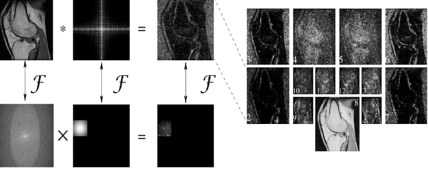
Fig. 3. A graphical example of sub-band filtering. The top row corresponds to the spatial domain and the bottom row the Fourier domain. Once slice from a knee MRI data set is filtered with a sub-band filter with a particular frequency and orientation by a product in the Fourier domain, which is equivalent to a convolution in the spatial domain. The filtered image becomes one measurement of the space,S2 in this example.
space S in its frequency and spatial domains is then defined as:
Si
w(ρ, κ, ς) = Fωi(ρ, κ, ς) Vω(ρ, κ, ς)
Si = |F−1[Si
ω]|, (3)
where(ρ, κ, ς)are the co-ordinates in the Fourier domain. At the next level, the coordinates(L1
r(1)×L1c(1)×L1s(1))
will become(Lr(2)×Lc(2)×Ls(2))with dimensionsNr(2) = Nr2(1), Nc(2) = Nc2(1), Ns(2) = Ns2(1). It is assumed thatNr(1) = 2a, Nc(1) = 2b, Ns(1) = 2c so that the results of the divisions are always integer values. To illustrate the OP on a textured image, a 2D example is presented in Figure 3.
V. FEATURE SELECTIONUSING THEBHATTACHARYYA SPACE
The sub-band filtering of the textured data produces a series of measurements that belong to a measurement
spaceS. Whether this space corresponds to the results of filters, features of the co-occurrence matrix or wavelets, not all the dimensions will contribute to the discrimination of the different textures that compose the original data. Besides the discrimination power that some measurements have, there is an issue of complexity related to the number of measurements used. Each extra texture feature may enrich the measurement space but will also further burden any subsequent classifier. Another advantage of selecting a subset of the space is that it can provide a better understanding of the underlying process that generated the data [41].
A common method of forward feature selection is the wrapper approach [42], [43]. This approach uses the error rate of the classifier itself as the criterion to evaluate the features selected, using a greedy selection, either hill
climbing, or best-first and treats the measurements as a search space organization: a representation where each state
is a measurement. It is important to bear in mind two issues: one is that hill climbing can lead to local optima, and the other is that the strength of the algorithm – the use of the classifier in the selection process instead of other evaluation functions – is at the same time its weakness, since the classification process can be slow.
[image:5.612.100.516.139.304.2]number of classifications which remain for every new feature is significantly reduced. In order to obtain a quantitative measure of class separability, a distance measure is required. With the assumption about the underlying distributions, a probabilistic distance can be easily extracted from some parameters of the data. Kailath [45] compared the Bhattacharyya distance and the Divergence (Kullback-Leibler), and observed that Bhattacharyya distance yields better results in some cases while in other cases they are equivalent. A recent study [18] considered a number of measures: Bhattacharyya, Euclidean, Kullback-Leibler, Fisher, for texture discrimination and concluded that the Bhattacharyya distance is the most effective texture discriminant for sub-band filtering schemes.
In its simplest formulation, the Bhattacharyya distance [46] between two classes can be calculated from the variance and mean of each class in the following way:
DB(k1, k2) = 1 4ln
1 4(
σk2
1 σ2 k2 +σ 2 k2 σ2 k1 + 2) ! +1 4
(µk1−µk2) 2
σ2
k1+σ
2
k2
!
, (4)
where DB(k1, k2) is the Bhattacharyya distance between two different training classes k1 and k2, and µk1, σk1 and µk2, σk2 correspond to the mean and variance of each one.
The Mahalanobis distance is a particular case of the Bhattacharyya distance, when the variances of the two classes are equal; this eliminates the first term of the distance that depends solely on the variances of the distribution. If the variances are equal this term will be zero, and grows as the variances differ. The second term, on the other hand, will be zero if the means are equal and is inversely proportional to the variances.
The Bhattacharyya space,B(i, p), is defined on the measurement space S as:
Lp×Li;B(i, p) :Lp×Li →DB(Ski1, S
i
k2). (5)
where each class pair,p, between classesk1, k2at measurementiwill have a Bhattacharyya distanceDB(Ski1, Ski2), and will produce a Bhattacharyya space of dimensions Np = (N2k) and Ni = 7o :Np×Ni (2D). The domains of the Bhattacharyya space are Li ={1,2, . . .7o} and Lp ={(1,2),(1,3), . . .(k1, k2), . . .(Nk−1, Nk)} where o is the order of the OP. In the volumetric case, Lp remains the same (since it depends on the classes only),Ni = 29o and Li ={1,2, . . .29o}.
The marginal distributions ofB(i, p) are
BI(i) =
Np
X
p=1
B(i, p) =
Np
X
p=1
DB(Ski1, S
i
k2), i= 1, . . . , Ni, (6)
BP(p) =
Ni
X
i=1
B(i, p) =
Ni
X
i=1
DB(Ski1, S
i
k2), p= 1, . . . , Np. (7)
The marginal over the class pairs,BI(i)sums the Bhattacharyya distances of every pair of a certain feature and thus will indicate how discriminant a certain sub-band OP filter is over the whole combination of class pairs. Whereas the marginal BP(p) sums the Bhattacharyya distances for a particular pair of classes over the whole measurement space and reveals the discrimination potential of particular pairs of classes when multiple classes are present.
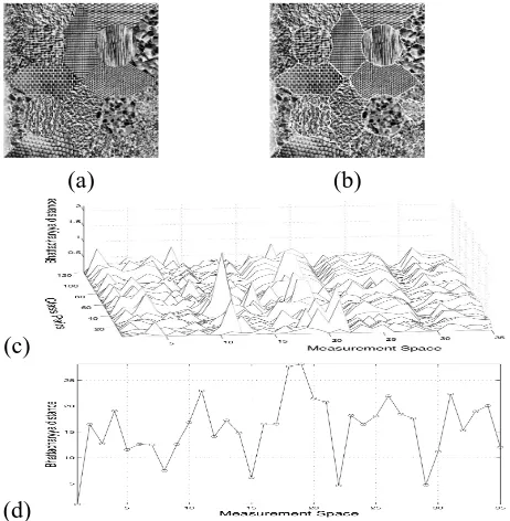
(a) (b)
(c)
[image:7.612.190.421.24.260.2](d)
Fig. 4. (a) 16-class natural texture mosaic (image f from Randen [27]). (b) Classification result using BS selected features. Average classification error is 16.5%. (c) The Bhattacharyya spaceB for a measurement spaceS of order 5 from the 16-texture image. (d) Marginal
BI(i), the index Measurement Space corresponds to spaceS.
constructed on training data and the individual Bhattacharyya distances are calculated between pairs of classes. Therefore, there is no guarantee that the feature selected will always improve the classification of the whole data space, the features selected could be mutually redundant or may only improve the classification for a pair of classes but not the overall classification [47]. Thus the conjecture to be tested then is whether the classification can be improved in a best-first, sequential selection defined by the Bhattacharyya space order statistics. The natural textures image was classified with several sequential selection strategies:
• Following the unsorted order of the measurement space: S1, S2, S3 etc. • Following the marginal BI(i) in decreasing order: S19, S18, S11 etc.
• Following the marginal BI(i) in increasing order: S28, S21, S15 etc. (The converse conjecture is that the
reverse order should provide the worst path for the classification.)
• Three random permutations.
The sequential misclassification results of the previous strategies are presented in Figure 5 where the advantage of the route provided by the B(I) can be seen. If extra time can be afforded, then the training data can be used with a more elaborate feature selection strategy; various forward and backward optimizations are possible (see [47]). Our experiments on 2D texture mosaics, however, have not shown a significant benefit by these methods in the final classification error over the sub-optimal best-first approach used here [44], [48], and we have demonstrated superior performance over other techniques: Local Binary Pattern (LBP) and the p8 methods presented by Ojala [49]; and wavelet features with the Watershed transformation presented by Malpica [50].
Fig. 5. Misclassification error for the sequential inclusion of features to the classifier for the 16-class natural textures image (figure 4 (a)). The route provided by the ordered marginalsB(I)(i)yields the best classification strategy.
[image:7.612.204.414.576.662.2]a predetermined number of features as the reduced set or sub-space used for classification. This can be particularly useful in cases where it can be computationally expensive to calculate the entire measurement space. Then, based on the training data, only a few measurements need to be generated based on the first n features of the B.
VI. MULTIRESOLUTION CLASSIFICATION
This section presents a new multiresolution algorithm, Multiresolution-Volumetric Texture Segmentation (M-VTS). The multiresolution procedure consists of three main stages: the process of climbing the levels or stages of a pyramid or tree, a decision or classification at the highest level is performed, and the process of descending from the highest level down to the original resolution. Based on the decision-directed approach of Wilson and Spann [1], we replace the contextual boundary-refinement step at each scale with a steerable-filter based on butterfly neighborhoods [19]. This is a satisfactory compromise over the use of a multiresolution MRF to gain a notion of contextual label smoothing but avoids the need to model and estimate a complicated set of boundary priors over 3D neighborhoods [51].
Smoothing the measurement space can improve the classification results; many isolated elements disappear and regions are more uniform. But a new problem arises with smoothing, especially at the boundaries between textures. When the measurement values of elements that belong to the same class are averaged, it is expected that they will tend to the class prototype, but if the elements belong to different classes, the smoothing can place them in a different class altogether. It would be ideal to smooth selectively depending on the distance to the boundaries. Of course, the class boundaries need then to be known. A compromise has to be reached between the intra-class smoothing and the class boundary estimation. A solution to this problem is to apply a multiresolution procedure of smoothing several levels with a pyramid before estimating the boundaries at the highest level and applying a boundary refinement algorithm in the descent to the highest resolution.
A. Smoothing the Measurement Space
The climbing stage represents the decrease in resolution of the data by means of averaging a set of neighbors on one level (children elements or nodes) up to a parent element on the upper level. Two common climbing methods are the Gaussian Pyramid [52] and the Quad tree ([53], [54], [55]). In our implementation we used the quad tree structure which, in 3D, becomes an oct tree (OT). The decrease in resolution correspondingly reduces the uncertainty in the elements’ values since they tend toward their mean. In contrast, the positional uncertainty increases at each level [1].
The measurement spaceS constitutes the lowest level of the tree. For each measurementSi of the space, a OT is constructed. To climb a level in the OT, a REDU CE operation is performed [52]:
(Si)L=REDU CE(Si)L−1, (8) where L is the level of the tree.
EveryREDU CE step averages eight contiguous elements to produce a single element in the upper level. Once a desired level is reached, the classification is performed.
B. Classification
At the highest level, the new reduced space can be classified. Partitioning of the measurement space can be considered as a mapping operator
λ:S→ {1,2, . . . , Nk}, (9) where the clusters or classes are λ−1(1), λ−1(2), ..., and these are unknown. Then, for every element x ∈S, λ
a will be an estimator for λ where, for every class, there is a point{a1, a2, . . .} ∈S such that these points define hyperplanes perpendicular to the chords connecting them, and split the space into regions {R1, R2, . . .}. These regions define the mapping function λa :S → {1,2. . . , Nk} by λa(x) = K if x ∈ RK, K = 1,2, ..., NK. This partitioning should minimize the Euclidean distance from the elements of the space to the points a, expressed by [56]:
ρ(a1, a2, . . .) =
X
x∈(Lr×Lc×Ls)
min 1≤j≤Nk
The measure of closeness of the estimator λa to λdefines a misclassification error by [λa] =P(λa(x)6=λ(x)), and P(λa(S) 6= λ(S)) for an arbitrary point x ∈ S in the space. If the values of the points ak are known, or there is a way of estimating these from training data, the classification procedure is supervised, otherwise it is
unsupervised. For this work, the points in the measurement space ak were obtained by filtering separate training data with the OP. Once the measurement space S is calculated for every training image, the average can be used as an estimate of the mean of the class:aˆk and equation 10 can be minimized by an iterative method such nearest neighbor (NN) clustering. In the experiments presented below, where supervised classification was required we used a NN approach.
C. Boundary Refinement
To regain full spatial resolution at the lowest level of the tree, the classification at the higher level has to be propagated downward. The propagation implies that every parent bequeaths: (a) its class value to 8 children and; (b) the attribute of being or not being in a boundary (figure 6). Interaction between neighbors can reduce the uncertainty in spatial position that is inherited from the parent node. This process is known as spatial restoration and boundary refinement, which is repeated at every stage until the bottom of the tree or pyramid is reached.
[image:9.612.198.413.242.363.2](a) (b)
Fig. 6. Inheritance of labels to child elements: (a) Class inheritance; (b) Boundary inheritance.
Butterfly filters (BF) [19] are orientation-adaptive filters, that consist of two separate sets or wings with a pivot element between them. It is the pivot element x = (r, c, s) which is modified as a result of the filtering. Each of the wings will have a roughly triangular shape , which resembles a butterfly (figure 7 (a)) and they can be regarded as two separate sets of anisotropic cliques, arranged in a steerable orientation. We propose the extension of these BF filters into 3D, and two possible shapes can be used: pyramidal or conic (figure 7 (b,c)), for ease of implementation we used pyramidal. The boundary determined by the classification process defines the orientation of the filter which places each of the wings of the butterfly to either side of the boundary. When dealing with volumes and not images, the boundaries between classes are not single lines but planes, and therefore the orientation of the butterflies requires two parameters, θandφ. We quantized each orientation in four steps:θ, φ={0,π4,π2,34π}. The elements covered by each of the wings are included in the filtering process while the values of the elements along the boundary (which are presumed to have greater uncertainty) and the pivot, x, are not included in the smoothing process. The BF consists of two sides, with left and right wings: lw/rw, each of which comprises Nw elements:
lw = {lw1, lw2, . . . , lwNw}
rw = {rw1, rw2, . . . , rwNw}
lw, rw∈S. (11)
(a) (b) (c)
Fig. 7. (a) 2D Butterfly filter, (b) Pyramidal volumetric butterfly filters, (c) Conic volumetric butterfly filters. Orientation of φ and θ
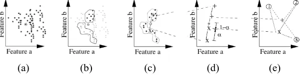
[image:9.612.190.525.560.693.2](a) (b) (c) (d) (e)
Fig. 8. A feature space view of boundary refinement process with butterfly filters. (a) A boundary elementxwith other elements. (b)x
and the two sets of neighboring elements that are comprised by the butterfly wings, all other elements are not relevant at this moment. (c) The weighted average of each wing. (d) Parameter αbalances between the elementxand the average of the wings. (e) New positions are compared with the prototypes (1,2,. . . ,k) of the classes, the class that corresponds to the minimum distance is then assigned tox.
For each wing, an average of the values of the elements in each dimension is calculated:
˜
Silw(x) = 1
Nw
Nw
X
q=1
Si(lwq), S˜rwi (x) =
1
Nw
Nw
X
q=1
Si(rwq). (12)
The actual pivot element x= (r, c, s) value is then combined with the mean values as follows: ˜
Sx−lw = (1−α)S(x) + αS˜lw, (13)
˜
Sx−rw = (1−α)S(x) + αS˜rw. (14) where α is a scalar gain measure that depends on the dissimilarity of the distribution of the elements that make up the wings:
α= 1
1 +e(5−D), D=
|S˜lw−S˜rw|
q
σ2lw+σ2
rw
, (15)
where σ2
lw and σrw2 are the variances of the elements in each butterfly wing.
The parameter α acts as weighting factor of the distance between the distributions covered by the two sides of the butterfly filter, and provides a balance between the current value of the element and a new one calculated from its neighbors. It is interesting to note that this balancing procedure is similar to the update rule of the Kohonen Self Organizing Maps [57].
The distance measure between the updated pivot element and the prototype values of each class determines to which class it is reassigned. Figure 8 shows the process graphically. At the classification stage, the new feature values
˜
Sx−lw,S˜x−rw replace the original feature values of element x. Instead of looking for a class based on λa(S(x)), the new valuesλa( ˜Sx−lw)/λa( ˜Sx−rw)will determine the class according to its closeness to class prototypes (using the mapping operator λa from equation 9).
VII. EXPERIMENTAL RESULTS
A. 3D Artificial Textures
There are many examples test images available for comparing 2D texture segmentation methods. However, up to the best of the authors’ knowledge, there is not such a database for volumetric texture. We have therefore created a handful of 3D data sets to demonstrate and compare the performance of the presented algorithm and measurement extraction techniques. First, a volumetric set that represents a simple two-class measurement space, each with 32×16×32elements drawn from Gaussian distributions (Class A:S1 µ
1 = 25, σ1= 2,S2 µ2= 26, σ2 = 4, Class B: S1 µ
1 = 27, σ1 = 7, S2 µ2 = 28, σ2 = 7). The two classes together form a 32×32×32×2 space. The data was classified unsupervised with the number of classes provided but not the estimates of the means. First it was clustered with the Linde-Buzo-Gray vector quantization method (LBG) [58] in a single resolution and then using M-VTS (OT levelL = 3). The classification results are presented in Figure 9 as clouds of points for each class for M-VTS. Results are presented in Table I. With M-VTS there are some incorrectly classified voxels close to the boundary, but the general shape of the original data is preserved and its overall error rate is much lower.
and S3, and classification was again performed unsupervised for single and multiresolution. Results are presented in Table I.
Again, some voxels near the boundary are misclassified, less than 3%, but the shape (figure 9 (c)) is well preserved. The computational complexity was considerably increased in 3D, for the first set the respective times for LBG and M-VTS were 0.1s and 14.9s and for the second set 0.4s and 54.0s.
[image:11.612.214.405.243.325.2](a) (b) (c)
Fig. 9. Classification of 3D textures: (a,b) Class 1 and Class 2 (figure 1 (a)), (c) Both classes (figure 1 (b)).
Algorithm
Data LBG M-VTS L= 3
Gaussian Data 14.1 6.2
Oriented Data 4.6 3.0
Knee Phantom 13.0 7.0
TABLE I
MISCLASSIFICATION(%)FORLBGANDM-VTSFOR THE SYNTHETIC3DTEST SETS.
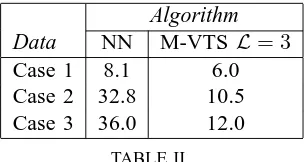
Algorithm
Data NN M-VTS L= 3
Case 1 8.1 6.0
Case 2 32.8 10.5
Case 3 36.0 12.0
TABLE II
SUMMARY OF MISCLASSIFICATION(%)FORNN (AT FULL RESOLUTION)ANDM-VTSFOR THEMRIKNEE DATA.
B. 3D Synthetic Knee Phantom
[image:11.612.232.386.377.458.2](a) (b) (c)
Fig. 10. Synthetic knee phantom image size128×128×128consisting of 4 texture types arranged approximately into background, bones, muscle and other. (a) 3D visualization of the original data. (b) Arrangement of principal regions in volume. (c) 3D visualization of labeled data.
(a) (b) (c) (d)
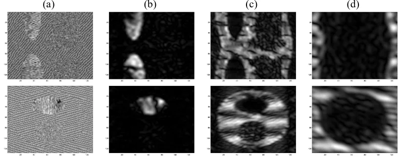
Fig. 11. (a) Knee phantom data, saggital slice 70 (top-row) and axial slice 110 (bottom-row). (b)-(d): First three most relevant features from OP of knee phantom (S54, S18, S64) shown as cross-sectional views.
C. 3D MRI texture segmentation
A set of experiments was conducted with 3D MRI sets of human knees acquired under different protocols: one set with Spin Echo and two sets with SPGR. In the three cases each slice had dimensions of 512×512 pixels and 87, 64 and 60 slices respectively. One sample slice from each set is presented in Figure 14 (a). The bones, background, muscle and tissue classes were hand labeled to provide ground-truth for evaluation.
For the first data set, Case 1, the following classification approach was followed. Four training regions of size 32×32×32elements were manually selected for the classes of background, muscle, bone and tissue. These training regions were small relative to the size of the data set, and they remained as part of the test data. Each training sample was filtered with the OP sub-band filtering scheme, and the results were used to construct the Bhattacharyya space (figure 13 (a)).
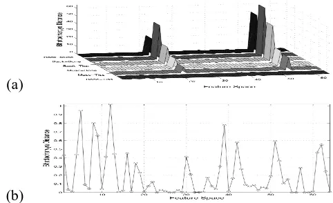
It can be immediately noticed that two bands: S22,54, which correspond to the low pass bands, dominate the discrimination while the distance of the pair bone-tissue is practically zero compared with the rest of the space. If the marginals are calculated directly the low pass would dominate and the discrimination of the bone and tissue classes, which are difficult to segment, would not be possible. Figure 13 (b) zooms into the Bhattacharyya space of the bone-tissue pair. Here we can see that some features: S12,5,8,38,..., provide discrimination between bone and tissue, and the low pass bands help discriminate the rest of the classes.
Feature selection was performed with the Bhattacharyya space and 7 measurements were selected: S22 and
[image:12.612.105.507.172.331.2](a)
[image:13.612.192.423.31.178.2](b)
Fig. 12. (a) MarginalBI(i)of knee phantom features space from OP. (b) Classification error comparing LBG against M-VTS at L= 3
and L= 4for sequential selection of features based on the BS feature selection. M-VTS is has consistently lower misclassification errors (about half of LBG with 3 or more features).
(a)
[image:13.612.183.424.248.395.2](b)
Fig. 13. Knee MRI: (a) Bhattacharyya spaceB (3D, order 2), (b) Bhattacharyya space (Bi(bone, tissue)).
(a) (b) (c)
[image:13.612.190.429.435.673.2]TABLE III
CLASSIFICATION(%)OFBONE(˜b)ACCORDING TO THE MASK FOR BONE(b)WITH K-MEANS,ANDM-VTS. FORCASE3,SUPERVISED AND UNSUPERVISED CLASSIFICATION WAS PERFORMED.
Knee Set Algorithm ˜b∈b ˜b∈(b)c (˜b)c ∈b (˜b)c ∈(b)c
Case 2 LBG (UnSup) 67.2 21.0 32.8 79.0
M-VTS (Sup) 89.5 21.6 10.5 78.4
Case 3 LBG (UnSup) 42.2 22.9 57.8 77.1
ˆ
ak (Sup) 64.0 11.0 36.0 89.0
M-VTS (UnSup) 75.8 3.5 24.2 96.5
M-VTS (Sup) 88.0 7.1 12.0 92.9
The SPGR MRI data sets were classified and the bone was segmented with the objective of using this as an initial condition for extracting the cartilage of the knee. The cartilage adheres to the condyles of the bones and appears as a bright, curvilinear structure in SPGR MRI data.
Besides the low pass,S22, three high frequency bands were selected, namely S1,5,9.
The performance of the classification schemes was measured on the ability to correctly classify the bone since this class alone will be used to segment the cartilage later on in this section. The correct classification was measured by how much bone was classified correctly inside the bone mask (˜b∈b), and how much bone was classified outside the bone mask (˜b ∈(b)c) and their complements ((˜b)c ∈ b , (˜b)c ∈(b)c). The knee was classified with LBG and M-VTS at level 3. One slice of the classified results is presented in the middle row of figure 14. As expected, M-VTS presents smoother results and reduces the misclassification of the bone from 32.8% to 10.5%. For Case 3 (bottom row of Figure 14) the reduction was from 57.8% to 24.2% with the unsupervised LBG method and if training data was used, the misclassification went down from 36.0% down to 12.0% with NN (table III).
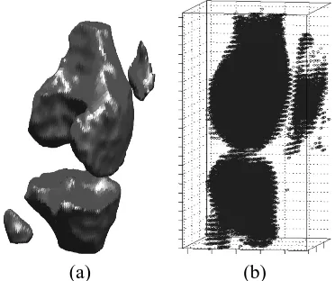
Figure 15 (a) presents a volume rendering of the segmented bone of Case 1. The four boney structures present in the MRI data set are clearly identifiable: patella, fibula, femur and tibia, and (b) shows a cloud of points of the bone class of Case 3. Here the misclassification is noticeable in the upper part of the patella (knee-cap), which is classified as background, and the lower part extends more than it should do into surrounding soft tissue (the infrapatellar pad).
(a) (b)
Fig. 15. (a) Rendering of the segmented bone of Case 1 (misclassification 8.1%) and (b) the segmented bone˜b(as clouds of points) from Case 3 (misclassification 12.0%).
D. Segmentation of the cartilage
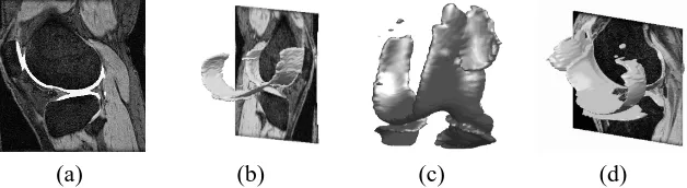
[image:14.612.213.399.439.595.2](a) (b) (c) (d)
Fig. 16. Cartilage of Case 2: (a) Slice 15 of the set with the cartilage in white, (b) Rendering of the cartilage and one slice of the MRI Set. Cartilage of Case 3: (c) Rendering of the cartilage, (d) The cartilage and one slice of the MRI set.
In this section, we propose a simple technique to extract the cartilage without the use of deformable models. The user has to determine a Region of Interest (ROI) and a gray level threshold with the bone extracted from the previous section being used as a starting point. In order to segment the cartilage out of the MRI sets, two heuristics were used: cartilage appears bright in the SPGR MRIs, and cartilage resides in the region between bones. This is translated into two corresponding rules: threshold voxels above a certain gray level, and discard those not close to the region of contact between bones. The methodology to extract the cartilage followed these steps: extract the boundary of the bone segmented by the M-VTS; dilate this boundary by a number of elements to each side (5 voxels in our case); eliminate the elements outside the ROI and the dilated boundary; threshold the region (gray levelg= 550for Case 2, andg= 280for Case 3); finally, eliminate isolated elements. It should be noted that the ROI is a cuboid and not an elaborate anatomical template.
Figure 16 presents the cartilage extracted from Cases 2 and 3. Some false positives can be seen, but the general shape is visually close to that of the cartilage. In these results, it is clear that the general shape of the cartilage; tibial, femoral and patellar is correctly segmented and the few incorrectly classified voxels could be easily erased from the result.
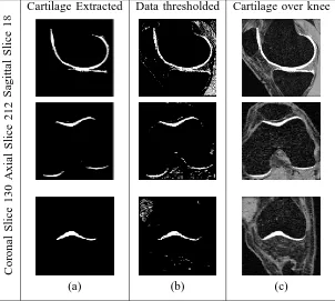
Figure 17 presents the segmented cartilage of Case 3 for three slices of the set in different view: sagittal slice 18, axial slice 212 and coronal slice 130. Figure 17 (a) presents the segmented cartilage. Some false positives appear as small dots in the image. The tibial cartilage also appears a bit ragged but the general shape is correct, notice for instance the separation of the patellar cartilage from the femoral cartilage. As a comparison, figure 17 (b) presents the thresholded data of the same slices. Figure 17 (c) presents the cartilage over the original image.
A last validation test was performed. The cartilage of figure 16 (a) was hand segmented and compared with the M-VTS results. Figure 18 shows the comparison as the sum of the number of pixels per row classified as cartilage with both techniques. It can be seen from the shape of both lines that the manual segmentation and the M-VTS are very similar.
VIII. CONCLUSIONS
A multiresolution algorithm based on Fourier domain filtering was presented for the classification of texture volumes. Textural measurements were extracted in 3D data by sub-band filtering with an Orientation Pyramid tessellation. Some of the measurements can be selected to form a new feature space and their selection is based on their discrimination powers obtained from a novel Bhattacharyya space. A multiresolution algorithm was shown to improve the classification of these feature spaces: oct trees were formed with the features. Once the classification is performed at the a higher level of the tree, the class and boundary conditions of the elements are propagated down. A boundary refinement method with pyramidal, volumetric butterfly filters is performed to regain spatial resolution.
The algorithm presented was tested with artificial 3D images, a phantom type artificial textured volumes and MRI sets of human knees (SPGR and Spin Echo). Satisfactory classification results were obtained in 3D at a modest computational cost.
Cartilage Extracted Data thresholded Cartilage over knee
S
ag
it
ta
l
S
li
ce
1
8
A
x
ia
l
S
li
ce
2
1
2
C
o
ro
n
al
S
li
ce
1
3
0
[image:16.612.156.458.25.296.2](a) (b) (c)
Fig. 17. Sagittal, coronal and axial view of the cartilage extracted from knee Case 3. The first column (a) shows the cartilage in the three planes, Second Column (b) shows the data thresholded at the same level used to extract the cartilageg= 280, the third column (c) shows the cartilage over the corresponding slice.
Fig. 18. M-VTS and manual segmentation comparison performed on the cartilage of figure 16 (a). The sum of number of pixels classified as cartilage in every row show good agreement of the M-VTS results with the manual segmentation.
Furthermore, there is manual intervention in determining the number of classes, the size of the butterfly filters, the depth of the OP decomposition and the height of the OT used by the coarse-to-fine refinement. Further research might be focused in these areas.
IX. ACKNOWLEDGEMENTS
Dr Simon Warfield provided some of the MRI data sets and also kindly reviewed the results. Professor Roland Wilson and Dr Nasir Rajpoot are acknowledged for their valuable discussions on this work and help in revising the manuscript. The test data sets along with the software are available on an “as is” basis on the author’s web page: http://www.dcs.warwick.ac.uk/∼creyes/m-vts.
REFERENCES
[1] R. Wilson and M. Spann, Image Segmentation and Uncertainty. New York: John Wiley and Sons Inc., 1988.
[2] T. Ojala, M. Pietik¨ainen, and D. Harwood, “A Comparative Study of Texture Measures with Classification based on Feature Distributions,” Patt Rec, vol. 29, no. 1, pp. 51–59, 1996.
[3] T. Reed and J. du Buf, “A Review of Recent Texture Segmentation and Feature Extraction Techniques,” CVGIP: Image Understanding, vol. 57, no. 3, pp. 359–372, May 1993.
[4] M. Tuceryan and A. K. Jain, “Texture Analysis,” in Handbook of Pattern Recognition and Computer Vision, C. H. Chen, L. F. Pau, and P. S. P. Wang, Eds. World Scientific Publishing, 1998, pp. 207–248.
[5] J. Weszka, C. Dyer, and A. Rosenfeld, “A Comparative Study of Texture Measures for Terrain Classification,” IEEE Trans. Syst., Man,
[image:16.612.200.414.345.416.2][6] V. A. Kovalev, M. Petrou, and Y. S. Bondar, “Texture Anisotropy in 3D Images,” IEEE Trans. Image Processing, vol. 8, no. 3, pp. 346–360, 1999.
[7] C. C. Reyes-Aldasoro and A. Bhalerao, “Volumetric Texture Description and Discriminant Feature Selection for MRI,” in Proceedings
of Information Processing in Medical Imaging, C. Taylor and A. Noble, Eds., Ambleside, UK, July 2003, pp. 282–293.
[8] M. Segovia-Mart´ınez, M. Petrou, V. A. Kovalev, and P. Perner, “Quantifying Level of Brain Atrophy Using Texture Anisotropy in CT Data,” in Medical Imaging Understanding and Analysis, Oxford, UK, July 1999, pp. 173–176.
[9] Y. Zhan and D. Shen, “Automated Segmentation of 3D US Prostate Images Using Statistical Texture-Based Matching Method,” in
MICCAI, Canada, November 16-18 2003, pp. 688–696.
[10] ——, “Deformable segmentation of 3-D ultrasound prostate images using statistical texture matching method,” IEEE Trans. Med. Imag., vol. 25, no. 3, pp. 256– 272, 2006.
[11] E. A. Hoffman, J. M. Reinhardt, M. Sonka, B. A. S., J. Guo, O. Saba, D. Chon, S. Samrah, H. Shikata, J. Tschirren, K. Palagyi, K. C. Beck, and G. McLennan, “Characterization of the Interstitial Lung Diseases via Density-Based and Texture-Based Analysis of Computed Tomography Images of Lung Structure and Function,” Academic Radiology, vol. 10, no. 10, pp. 1104–1118, 2003. [12] A. Carrillat, T. Randen, L. Sønneland, and G. Elvebakk, “Seismic stratigraphic mapping of carbonate mounds using 3D texture attributes,”
in Extended Abstracts, Annual Meeting, European Association of Geoscientists and Engineers, Florence, Italy, May 27-30 2002. [13] T. Randen, E. Monsen, A. Abrahamsen, J. O. Hansen, J. Schlaf, and L. Sønneland, “Three-dimensional texture attributes for seismic
data analysis,” in Ann. Int. Mtg., Soc. Expl. Geophys., Exp. Abstr., Calgary, Canada, August 2000.
[14] C. Tai and K. Baba-Kishi, “Microtexture Studies of PST and PZT Ceramics and PZT Thin Film by Electron Backscatter Diffraction Patterns,” Textures and Microstructures, vol. 35, no. 2, pp. 71–86, 2002.
[15] W. M. Wells, W. E. L. Grimson, R. Kikinis, and F. A. Jolesz, “Adaptive Segmentation of MRI Data,” IEEE Trans. Med. Imag., vol. 15, no. 4, pp. 429–442, 1996.
[16] M. Styner, C. Brechb¨uler, G. Sz´ekely, and G. Gerig, “Parametric estimate of intensity inhomogeneities applied to MRI,” IEEE Trans.
Med. Imag., vol. 19, no. 3, pp. 153–165, 2000.
[17] A. Bhalerao and C. Reyes-Aldasoro, “Volumetric Texture Description and Discriminant Feature Selection for MRI,” in Proceedings of
Eurocast’03, Canarias, Spain, February 2003.
[18] A. Bhalerao and N. Rajpoot, “Selecting Discriminant Subbands for Texture Classification,” in BMVC, Norwich, UK, September 2003. [19] P. Schroeter and J. Bigun, “Hierarchical Image Segmentation by Multi-dimensional Clustering and Orientation-Adaptive Boundary
Refinement,” Patt Rec, vol. 28, no. 5, pp. 695–709, 1995.
[20] R. M. Haralick, “Statistical and Structural Approaches to Texture,” Proceedings of the IEEE, vol. 67, no. 5, pp. 786–804, 1979. [21] G. R. Cross and A. K. Jain, “Markov Random Field Texture Models,” IEEE Trans. Pattern Anal. Machine Intel., vol. 5, no. 1, pp.
25–39, 1983.
[22] J. M. Keller and S. Chen, “Texture Description and Segmentation through Fractal Geometry,” Computer Vision, Graphics and Image
Processing, vol. 45, no. 2, pp. 150–166, 1989.
[23] M. Unser, “Texture Classification and Segmentation Using Wavelet Frames,” IEEE Trans. Image Processing, vol. 4, no. 11, pp. 1549– 1560, 1995.
[24] S. Livens, P. Scheunders, G. V. de Wouwer, and D. V. Dyck, “Wavelets for texture analysis, an overview,” in 6th Int. Conf. on Image
Processing and its Aplplications, vol. 2, Dublin, Ireland, july 1997, pp. 581–585.
[25] M. Unser and M. Eden, “Multiresolution Feature Extraction and Selection for Texture Segmentation,” IEEE Trans. Pattern Anal.
Machine Intel., vol. 11, no. 7, pp. 717–728, 1989.
[26] L. Blot and R. Zwiggelaar, “Synthesis and Analysis of Solid Texture: Application in Medical Imaging,” in Texture 2002: 2nd Int
Workshop on Texture Analysis and Synthesis, Copenhagen, 1 June 2002, pp. 9–14.
[27] T. Randen and J. H. Husøy, “Filtering for Texture Classification: A Comparative Study,” IEEE Trans. Pattern Anal. Machine Intel., vol. 21, no. 4, pp. 291–310, 1999.
[28] R. Wilson and M. Spann, “Finite Prolate Spheroidal Sequences and Their Applications: Image Feature Description and Segmentation,”
IEEE Trans. Pattern Anal. Machine Intel., vol. 10, no. 2, pp. 193–203, 1988.
[29] P. de Rivaz and N. G. Kingsbury, “Complex Wavelet Features for Fast Texture Image Retrieval,” in Proc. ICIP, 1999, pp. 109–113. [30] Z. Lang, R. Scarberry, Z. Zhang, W. Shao, and X. Sun, “A texture-based direct 3D segmentation system for confocal scanning
fluorescence microscopic images,” in Twenty-Third Southeastern Symposium on System Theory, Columbia, SC, 10-12 March 1991, pp. 472–476.
[31] H. H. S. Ip and S. W. C. Lam, “Using an octree-based rag in hyper-irregular pyramid segmentation of texture volume,” in Proceedings
of the IAPR Workshop on Machine Vision Applications, Kawasaki, Japan, December 13-15 1994, pp. 259–262.
[32] R. A. Lerski, K. Straughan, L. R. Schad, D. Boyce, S. Bluml, and I. Zuna, “MR Image Texture Analysis - An Approach to tissue Characterization,” Mag Res Imag, vol. 11, no. 6, pp. 873–887, 1993.
[33] L. R. Schad, S. Bluml, and I. Zuna, “MR Tissue Characterization of Intracranial Tumors by means of Texture Analysis,” Mag Res
Imag, vol. 11, no. 6, pp. 889–896, 1993.
[34] COST European Cooperation in the field of Scientific and Technical Research, COST B11 Quantitation of Magnetic Resonance Image
Texture. http://www.uib.no/costb11/: World Wide Web, 2002.
[35] D. James, B. D. Clymer, and P. Schmalbrock, “Texture Detection of Simulated Microcalcification Susceptibility Effects in Magnetic Resonance Imaging of the Breasts,” J of Mag Res Imag, vol. 13, no. 6, pp. 876–881, 2002.
[36] T. Kapur, “Model-based three dimensional Medical Image Segmentation,” Ph.D. dissertation, AI Lab, Massachusetts Institute of Technology, May 1999. [Online]. Available: http://www.ai.mit.edu/people/tkapur/publications.html
[37] N. Saeed and B. K. Puri, “ Cerebellum Segmentation Employing Texture Properties and Knowledge based Image Processing : Applied to Normal Adult Controls and Patients,” Mag Res Imag, vol. 20, no. 5, pp. 425–429, 2002.
[39] V. A. Kovalev, F. Kruggel, and D. Y. von Cramon, “Gender and age effects in structural brain asymmetry as measured by MRI texture analysis,” NeuroImage, vol. 19, no. 3, pp. 895–905, 2003.
[40] J. M. Mathias, P. S. Tofts, and N. A. Losseff, “Texture Analysis of Spinal Cord Pathology in Multiple Sclerosis,” Magnetic Resonance
in Medicine, vol. 42, no. 5, pp. 929–935, 1999.
[41] I. Guyon and A. Elisseeff, “An Introduction to Variable and Feature Selection,” J of Machine Learning Research, vol. 3, no. 7-8, pp. 1157–1182, 2003.
[42] M. Dong and R. Kothari, “Feature subset selection using a new definition of classifiability,” Patt Rec Letts, vol. 24, no. 9-10, pp. 1215–1225, 2003.
[43] R. Kohavi and G. H. John, “Wrappers for feature subset selection,” Artificial Intelligence, vol. 97, no. 1-2, pp. 273–324, 1997. [44] C. Reyes-Aldasoro and A. Bhalerao, “The Bhattacharyya space for feature selection and its application to texture segmentation,” Patt
Rec, vol. 39, no. 5, pp. 812–826, 2006.
[45] T. Kailath, “The Divergence and Bhattacharyya Distance Measures in Signal Selection,” IEEE Trans. Commun. Technol., vol. 15, no. 1, pp. 52–60, 1967.
[46] G. B. Coleman and H. C. Andrews, “Image Segmentation by Clustering,” Proceedings of the IEEE, vol. 67, no. 5, pp. 773–785, 1979. [47] J. Kittler, “Feature Selection and Extraction,” in Handbook of Pattern Recognition and Image Processing, Y. Fu, Ed. New York:
Academic Press, 1986, pp. 59–83.
[48] C. C. Reyes-Aldasoro, “Multiresolution Volumetric Texture Segmentation,” Ph.D. dissertation, Department of Computer Science, University of Warwick, April 2005.
[49] T. Ojala, K. Valkealahti, E. Oja, and M. Pietik¨ainen, “Texture discrimination with multidimensional distributions of signed gray level differences,” Patt Rec, vol. 34, no. 3, pp. 727–739, 2001.
[50] N. Malpica, J. E. Ortu˜no, and A. Santos, “A multichannel watershed-based algorithm for supervised texture segmentation,” Patt Rec
Letts, vol. 24, no. 9, pp. 1545–1554, 2003.
[51] R. Wilson and C.-T. Li, “A Class of Discrete Multiresolution Random Fields and its Application to Image Segmentation,” IEEE Trans.
Pattern Anal. Machine Intel., vol. 25, no. 1, pp. 42–56, 2003.
[52] P. J. Burt and E. H. Adelson, “The Laplacian Pyramid as a compact Image Code,” IEEE Trans. Commun., vol. 31, no. 4, pp. 532–540, 1983.
[53] V. Gaede and O. G¨unther, “Multidimensional access methods,” ACM Computing Surveys, vol. 30, no. 2, pp. 170–231, 1998. [Online]. Available: citeseer.ist.psu.edu/gaede97multidimensional.html
[54] H. Samet, “The Quadtree and Related Hierarchical Data Structures,” Computing Surveys, vol. 16, no. 2, pp. 187–260, 1984.
[55] M. Spann and R. Wilson, “A quad-tree approach to image segmentation which combines statistical and spatial information,” Patt Rec, vol. 18, no. 3/4, pp. 257–269, 1985.
[56] E. R. Dougherty and M. Brun, “A probabilistic theory of clustering,” Patt Rec, vol. 37, no. 5, pp. 917–925, 2004. [57] T. Kohonen, Self-Organizing Maps, third extended ed. Berlin, Heidelberg, New York: Springer, 2001.
[58] Y. Linde, A. Buzo, and R. Gray, “An Algorithm for Vector Quantizer Design,” IEEE Trans. Commun., vol. 28, no. 1, pp. 84–95, 1980. [59] J. A. Lynch, S. Zaim, J. Zhao, A. Stork, C. G. Peterfy, and H. K. Genant, “Cartilage segmentation of 3D MRI scans of the osteoarthritic
knee combining user knowledge and active contours,” in Proceedings of SPIE, 2000.
[60] L. M. Lorigo, O. D. Faugeras, W. E. L. Grimson, R. Keriven, and R. Kikinis, “Segmentation of Bone in Clinical Knee MRI Using Texture-Based Geodesic Active Contours,” in MICCAI, Cambridge, USA, October 11-13 1998, pp. 1195–1204. [Online]. Available: citeseer.nj.nec.com/lorigo98segmentation.html
[61] S. K. Warfield, M. Kaus, F. A. Jolesz, and R. Kikinis, “Adaptive, Template Moderated, Spatially Varying Statistical Classification,”
Medical Image Analysis, vol. 4, no. 1, pp. 43–55, Mar 2000. [Online]. Available: citeseer.ist.psu.edu/warfield00adaptive.html
[62] I. van Breuseghem, “Ultrastructural MR imaging techniques of the knee articular cartilage: problems for routine clinical application,”