S
TRATHCLYDE
DISCUSSION PAPERS IN ECONOMICS
STOCHASTIC SEARCH VARIABLE SELECTION IN VECTOR
ERROR CORRECTION MODELS WITH AN APPLICATION
TO A MODEL OF THE UK MACROECONOMY
BY
MARKUS JOCHMANN, GARY KOOP, ROBERTO
LEON-GONZALEZ AND RODNEY W. STRACHAN
NO. 09-19
Stochastic Search Variable Selection in Vector
Error Correction Models with an Application
to a Model of the UK Macroeconomy
∗
Markus Jochmann
University of Strathclyde
Gary Koop
†University of Strathclyde
Roberto Leon-Gonzalez
National Graduate Institute
for Policy Studies
Rodney W. Strachan
University of Queensland
September 2009
Abstract
This paper develops methods for Stochastic Search Variable Selection (currently popular with regression and Vector Autoregressive models) for Vector Error Correction models where there are many possible strictions on the cointegration space. We show how this allows the re-searcher to begin with a single unrestricted model and either do model selection or model averaging in an automatic and computationally ef-ficient manner. We apply our methods to a large UK macroeconomic model.
Keywords: Bayesian, cointegration, model averaging, model selection, Markov chain Monte Carlo
JEL Codes: C11, C32, C52
∗All authors are Fellows at the Rimini Centre for Economic Analysis.
†Corresponding author: Gary Koop, Department of Economics, University of
1
Introduction
Empirical macroeconomic modelling is typically a complicated affair, involv-ing many time series variables. For instance, the UK macroeconomic models considered in this paper are based on the influential model of Garratt, Lee, Pesaran and Shin (2003, 2006), hereafter GLPS. This involves nine variables. Even if one remains in a conventional multivariate time series framework involving Vector autoregressive (VAR) and Vector error correction models (VECMs), there can be hundreds or more modelling choices. Some of these are driven by econometric considerations (e.g. choice of cointegrating rank, lag length, etc.) while others can be driven by economic theory considera-tions (e.g. GLPS develop a theoretical model of the UK macroeconomy which implies certain restrictions on the cointegrating relationships). In macroeco-nomic modelling exercises involving structural breaks, time variation in pa-rameters or regime switching such modelling choices proliferate (see, among many others, Primiceri, 2005 and Sims and Zha, 2006).
The challenge facing the empirical macroeconomist is how to navigate through this morass of choices. One common strategy, used by GLPS, is to select a single model. This can be done through sequential hypothesis testing procedures or by choosing the model with the highest value for an information criteria or marginal likelihood. Alternatively, economic theory can be used to guide model choice by giving special consideration to models consistent with a particular economic theory.
A second strategy is to do model averaging and present empirical results which are a weighted average over all models. Common choices for weights are marginal likelihoods or functions of information criteria. Empirical pa-pers adopting this approach include Sala-i-Martin, Doppelhoffer and Miller (2004), Fernandez, Ley and Steel (2001) and Koop, Potter and Strachan (2008). The literature is replete with extensive discussion of the compara-tive advantages and disadvantages of model averaging and model selection (e.g. Draper, 1995, Leamer, 1978, Raftery, Madigan and Hoeting, 1997). A problem with model averaging is that it can be extremely computationally demanding especially if, as in the current application, Markov Chain Monte Carlo (MCMC) methods are required to carry out inference in each model and the number of models is high.
de-scribed as working with a single very flexible model. The problems with such models are that they risk over-fitting and typically involve a large number of parameters which can be difficult to estimate with any precision. The solution to such problems is prior information. This prior information can be purely subjective or involve some data information (as in the classic Min-nesota prior for VAR models, see Doan, Litterman and Sims, 1984). Alterna-tively the prior can be hierarchical (i.e. can be expressed in terms of a set of unknown parameters which are estimated from the data). Indeed the state equations from state space models such as those used by Primiceri (2005) can be interpreted as hierarchical priors. The mixture innovation models of, e.g., Giordani and Kohn (2008) or Koop, Leon-Gonzalez and Strachan (2009b) can also be interpreted in this manner. Yet another recent hier-archical approach is explored and adapted in this paper. This is based on the Stochastic Search Variable Selection (SSVS) approach to VAR models developed in George, Ni and Sun (2008). The basic idea of this approach can be explained quite simply. Let λ be a parameter (e.g. a coefficient in a VAR). A conventional Bayesian approach would specify a prior for λsuch as λ ∼ N(0, Vλ). By setting Vλ to a large value, a relatively noninformative prior is obtained. Smaller values of Vλ will shrink the coefficient towards zero, something which has been found to be useful in many empirical appli-cations. Instead of such an approach, the SSVS prior is a hierarchical one, involving a mixture of two normal distributions:
λ∼(1−δ)N(0, Vλ0) +δN(0, Vλ1), (1)
where δ is a dummy variable which equals 0 if λ is drawn from the first normal and equals 1 if it is drawn from the second. The prior is hierarchical since δ is treated as an unknown parameter and estimated in a data-based fashion. The SSVS aspect of this prior arises by choosing the first prior variance, Vλ0, to be extremely “small” (so that the parameter is virtually zero) and the second prior variance,Vλ1, to be “large” (implying a relatively
noninformative prior for the parameter). The way in which “small” and “large” prior variances can be chosen is discussed in George, Ni and Sun (2008) and below.1
1
SSVS can be interpreted as working with a single very flexible model and then (in a data-based fashion) choosing a prior which ensures over-parameterization problems do not occur. But SSVS can also be used as a way of implementing the two strategies described above. The researcher can do model selection by selecting a single restricted model based on some metric involving δ(e.g. if Pr (δ= 1|Data)> 1
2 then the explanatory variable
corresponding to λ is included in the model, else it is excluded). Bayesian model averaging (BMA) can be done by using an unrestricted model with SSVS prior. This will implicitly average over models which include and ex-clude the explanatory variable associated withλ. The weights in this average will be Pr (δ= 1|Data) and Pr (δ= 0|Data), respectively.
The SSVS approach is very attractive for VAR modelling since VARs can have a large number of coefficients and many of them have no explana-tory power. For instance, the trivariate VAR(4) used in Jochmann, Koop and Strachan (2009) has 36 VAR coefficients and SSVS picks out only 10 of these as having important explanatory power. In such a situation, the number of hypothesis tests required in a sequential testing procedure could lead the researcher to serious worries about pre-test problems. Alternatively, the researcher who wants to select the single restricted VAR with highest marginal likelihood or highest value for an information criteria would face the serious problem of estimating at least 236 models (i.e. if each restricted
model is defined according to whether each of the 36 coefficients is included or excluded, the result is 236 models). Regardless of whether SSVS is used
for model selection or model averaging, it seems an attractive approach to VAR modelling which will shrink unimportant coefficients to zero and, thus, yield a much more parsimonious model. In essence, the SSVS prior can pick out restrictions automatically so that the researcher can begin with a flexible unrestricted model and let SSVS pick out the appropriate restrictions.
The major theoretical econometric contribution of this paper is to extend the SSVS approach, which is developed for multivariate normal linear models such as the VAR, to the nonlinear VECM. As we shall see, some subtle econometric issues arise in this regard. A related theoretical contribution is to extend the SSVS approach to restrictions other than ones like (1) where each coefficient is either included or excluded. In particular, macroeconomists such as GLPS are often interested in overidentifying restrictions involving several coefficients. We develop an SSVS approach which can pick out such restrictions automatically.
macroeconomic application involving a high dimensional model. The GLPS model fits the bill perfectly. It involves nine dependent variables, uncertainty over many modelling choices (e.g. cointegrating rank, lag length and treat-ment of deterministic terms) and many theoretical restrictions motivated by macroeconomic theory. We find SSVS to be computationally efficient and to lead to quite parsimonious modelling. We find support for interest rate parity and Fisher inflation parity conditions which are imposed by GLPS. However, we find less support for purchasing power parity and none at all for a restriction motivated by neoclassical growth models. These latter two restrictions are imposed by GLPS. Nevertheless, when we turn to impulse response analysis we find economically-sensible results which are not too dif-ferent than those of GLPS.
2
Models
A Bayesian model is defined by a likelihood function and a prior. We deal with each of these in turn in this section.
2.1
Likelihoods
The VECM for an n-dimensional vector, yt, is written as:
∆yt= Πyt−1+
p−1
X
j=1
Γj∆yt−j +µdt+εt (2)
for t = 1, .., T where the n×n matrix Π is of rank r ≤ n and dt denotes
deterministic terms. εt is i.i.d. N(0,Σ). The framework described in (2)
defines a set of models which differ in the number of cointegrating vectors (r), lag length (p) and the specification of deterministic terms. In addition, the researcher may wish to entertain various over-identifying restrictions on the cointegrating vectors.
The unrestricted VECM used in this paper, written in matrix form is:
Y =Xβα+WΓ +E, (3)
whereY isT×nwithtthrow given by ∆y′
t,X isT×(n+2) withtthrow given
by 1, t, y′ t−1
,βis (n+2)×rmax,αisrmax×n,W isT×[n(pmax−1) + 2] with tth row given by 1, t,∆y′
t−1, ..,∆yt′−p+1
T ×n withvec(E)∼N(0,Σ⊗I). rmax and pmax are the maximum number
of cointegrating relationships and lag length, respectively, that the researcher is willing to entertain. Note that, with regards to deterministic terms, a de-terministic trend in the cointegrating residuals has very different implications than a deterministic trend in the levels of the series. Accordingly, following Johansen (1995, Section 5.7), we potentially allow for deterministic terms in the cointegrating residual and directly in the conditional mean of ∆yt.
GLPS work with additional restrictions motivated by macroeconomic the-ory. A detailed explanation of this theory is provided in GLPS. Here we only sketch the details. The nine variables GLPS work with are the log of the oil price (po
t), the log of the effective exchange rate (et) , the
domes-tic and foreign nominal interest rates (it and i∗t), the inflation rate (∆pt),
the logs of domestic and foreign real per capita GDP (qt and qt∗), the log
of the ratio of domestic to foreign prices (pt − p∗t) and the log of the
ra-tio of real high powered money to real GDP per capita (ht − q). Thus,
yt = (pot, et, i∗t, it,∆pt, qt, pt−p∗t, ht−qt, qt∗)′. Exact definitions and sources
are given in the Data Appendix.
The model GLPS call their core model assumes five cointegrating rela-tionships of which the following four place restrictions on β. These are:
pt−p∗t −et=b1+e1t,
it−i∗t =b2+e2t,
qt−q∗t =b3+e3t,
it−∆pt =b4+e5t,
(4)
wherebiare intercepts in the cointegrating relationships andeit denote mean
zero stationary errors.2
GLPS derive and explain these cointegrating relationships in detail. Brief-ly, the first restriction is motivated by the purchasing power parity
relation-2
ship. The second from an interest rate parity condition. The third by neo-classical growth models for the UK and the rest of the world. The fourth is based on Fisher inflation parity arguments. These equations define over-identifying restrictions and we consider variants of our models which impose some or all of them.
In sum, we have so far developed a very general unrestricted model. How-ever, there are many restricted models of interest which differ in choice of p ≤ pmax, r ≤ rmax and the number of over-identifying restrictions imposed
(i.e. restrictions on the cointegration space). Furthermore, setting individual coefficients in α and/or Γ (if empirically warranted) would lead to the desir-able goal of a more parsimonious model. Note, in particular, that (3) allows for deterministic terms (both intercept and time trend) to enter both the cointegrating residual and ∆yt. Such a specification is typically too flexible
in macroeconomic empirical work and, thus, restricted models which zero out some of these deterministic terms are potentially of interest.
In most applications, this will lead to a huge model space. For instance, even if we ignore restrictions onα and/or Γ, if we setrmax= 5, pmax= 2 and
consider eighteen restrictions on β,3 we would have hundreds of models to
work with. This is the approximate number of models used in the conven-tional Bayesian cointegration analysis of Koop, Potter and Strachan (2008). Given that the methodology of Koop, Potter and Strachan (2008) required the running of an MCMC algorithm in each model, the computational re-quirements of that paper were quite substantial. In the present application, α is a 5×9 matrix and Γ an 11×9 matrix and, thus, in total they contain 144 parameters. If we are to extend our model space by considering models which allow for each individual element of α and/or Γ to be zero, then the number of models is further multiplied by 2144. Clearly, doing a
conven-tional Bayesian model selection or model averaging exercise which involves estimating each of more than 100×2144 models is computationally
impossi-ble. This consideration helps motivate our SSVS approach which, as we shall see, allows the researcher to work with the one model given in (3) and select appropriate restrictions in an automatic manner.
3
2.2
The SSVS Prior
In this paper, we will extend the SSVS prior for VARs of George, Ni and Sun (2008) to VECM models. The new econometric issues involve β and α. However, before describing our treatment of these parameters we will describe the prior for Γ and Σ. We do this since our treatment of Γ and Σ is exactly the same as George, Ni and Sun and, thus, we can introduce basic SSVS ideas in a familiar framework.
2.2.1 Prior for Γ and Σ
Note that, conditional on β and α, the VECM can be written as:
e
Y =WΓ +E, (5)
where Ye =Y −Xβα. This takes the form of a VAR and the SSVS methods for VARs of George, Ni and Sun (2008) can be applied directly in the context of an MCMC algorithm (except usingYe as the vector of dependent variables instead of Y).
SSVS can be interpreted as defining a hierarchical prior for Γ and Σ. Each element in the hierarchy is a mixture of two normals, one with a small variance (implying the coefficient is not in the model) and one with a large variance (implying the coefficient is included in the model). The SSVS prior for γ =vec(Γ) can be written as:
γ|δ∼N(0, D), (6)
where δ is a vector of unknown parameters with typical element δj ∈ {0,1},
and D is a diagonal matrix with the jth element given by κ2
j where
κ2j =
(
κ2
0j if δj = 0,
κ2
1j if δj = 1.
(7)
Note that this prior implies a mixture of two normals:
γj|δj ∼(1−δj)N 0, κ20j
+δjN 0, κ21j
, (8)
where γj is thejth element ofγ. δ is treated as a vector of unknown
param-eters and is estimated in a data based fashion. If δi = 0, then the prior for
zero. In this sense, we can say that, if δj = 0, then the jth explanatory
variable is excluded from the model (formally its coefficient is shrunk to be very near zero). If δj = 1, then the jth explanatory variable is included
and γj is estimated using a relatively noninformative prior. As discussed in the introduction, priors of this form can be used for model selection by choosing a single model which includes only those explanatory variables for which Pr (δi >1|Data)> c for some threshold c(e.g. c= 12). Alternatively,
Bayesian model averaging can be done by running the MCMC algorithm for the unrestricted model and simply averaging any feature of interest (e.g. an impulse response function or a predictive moment) over all MCMC draws. Since the MCMC algorithm provides draws of δ (as well as all other param-eters), this strategy amounts to averaging over models (i.e. in the sense that different drawn values forδdefine different models). Crucially, though, doing model averaging in this way requires only that the researcher run a single MCMC algorithm for the unrestricted model (as opposed running an MCMC algorithm in each restricted model).
We use what George, Sun and Ni (2008) call the “default semi-automatic approach” to selecting the prior hyperparameters κ2
0j and κ21j and the reader
is referred to their paper for additional justification for this approach. Basi-cally, κ2
0j should be selected so that γj is essentially zero and κ21j should be
selected so that γj is empirically substantive. The default semi-automatic
approach involves choosing κ2
0j = c0dvar γj
and κ2
1j = c1var γd j
where
d
var γj is an estimate of the posterior variance of the coefficient. In our empirical work, this is based on a preliminary MCMC run using a non-informative prior, although other estimates (e.g. based on maximum like-lihood estimation) are possible. The pre-selected constants c0 and c1 must
have c0 << c1 and we set c0 = 101 and c1 = 10.4
For δ, the SSVS prior posits that each element has a Bernoulli form (independent of the other elements of δ) and, hence we have
Pr (δj = 1) =qj,
Pr (δj = 0) = 1−qj. (9)
We set qj = 1
2 for all j. This is a natural default choice, implying each
4
coefficient is a priori equally likely to be included as excluded. For the error covariance matrix, we begin by decomposing it as:
Σ−1 = ΨΨ′, (10)
where Ψ is upper-triangular. The SSVS prior involves using a standard Gamma prior for the square of each of the diagonal elements of Ψ and the SSVS mixture of normals prior for each element above the diagonal. Note that this implies that the diagonal elements of Ψ are always included in the model, ensuring a positive definite error covariance matrix. This form for the prior also greatly simplifies posterior computation. Precise details are provided in the next paragraph.
Let the non-zero elements of Ψ be labelled as ψij and define ψ = (ψ11, .., ψnn)′, ηj = ψ1j, .., ψj−1,j
′
and η = (η′
2, .., η′n) ′
. For the di-agonal elements, we assume prior independence with
ψ2
jj ∼G aj, bj
, (11)
whereG aj, bj
denotes the Gamma distribution with mean aj
bj and variance aj
b2
j. We specify aj = 0.1 and bj = 0.001 which are relatively noninformative
choices, but center the prior at 100.0. The latter is a sensible value given the scale of the variables and the fact thatψ2
jj is the inverse of the error variance
in equation j.
The hierarchical prior forη takes the same mixture of normals form asγ. In particular, the SSVS prior has
ηj|ωj ∼N(0, Fj), (12)
where ωj = (ω1j, .., ωj−1,j)′ is a vector of unknown parameters with typical
element ωij ∈ {0,1}, and Fj =diag ξ21j, .., ξ2j−1,j
where
ξ2ij =
(
ξ20ij if ωij = 0,
ξ21ij if ωij = 1,
(13)
for j = 2, .., n and i = 1, .., j−1. Note that this prior implies a mixture of two Normals for each off-diagonal element of Ψ:
ψij|ωij ∼(1−ωij)N
0, ξ2 0ij
+ωijN
0, ξ2 1ij
As we did with κ2
0j and κ21j (the hyperparameters in the SSVS prior for
Γ), we use a semi-automatic default approach to selecting ξ20ij andξ21ij. That is, we set ξ20ij =c0dvar ψij
and ξ21ij =c1dvar ψij
, where dvar ψij is based on an estimate of the variance of the appropriate off-diagonal element of Σ. As with Γ, this estimate is obtained from a preliminary MCMC run using a non-informative prior. The pre-selected constants c0 and c1 are set (as
before) to be c0 = 101 and c1 = 10.
For ω = (ω′
2, .., ω′n) ′
, the SSVS prior posits that each element has a Bernoulli form (independent of the other elements of ω) and, hence, we have
Pr (ωij = 1) =qij,
Pr (ωij = 0) = 1−qij. (15)
We make the default choice of q
ij =
1
2 for all i and j.
The preceding material describes the basic ideas underlying SSVS and the details of how we implement it for Γ and Σ. SSVS has been found to be a very useful technique in finding parsimonious restricted versions of VARs. Posterior simulation methods are described in George, Ni and Sun (2008) and in Appendix A. Suffice it to note here that we use their algorithm to provide posterior draws of Γ, Σ , δ and ω (ω is the vector containing all the ωj) conditional on α and β.
2.2.2 Prior for α and β
SSVS has never been extended to VECMs. The fact thatβαenters in product form and the fact that (without further restrictions) the VECM only identi-fies the cointegrating space precludes the direct use of SSVS ideas for VARs. Before describing how SSVS can be implemented in a manner which over-comes these problems, we must digress and explain some basic issues which arise in Bayesian analyses of VECMs. An identification problem arises in the VECM since Π =βαand Π =βCC−1αare identical for any nonsingular C. In early work, a common practice was to impose a linear normalization
such as β =
Ir
β0
. However, a literature has recently emerged which
identifying restrictions places a restriction on the estimable region of the cointegrating space. Furthermore, a flat and apparently “noninformative” prior on β0 in the linear normalization strongly favors regions of the
coin-tegration space near where the linear normalization is invalid. Hence, the linear normalization is used under the assumption that it is valid while at the same time the prior puts weight near the region where the normalization is likely to be invalid. These considerations suggest that an alternative iden-tification restriction is required to form the basis for prior elicitation on the cointegration space. As shown in Strachan and Inder (2004) an identification restriction which does not suffer from the drawbacks of the linear and similar normalizations is:
β′β =I (16)
and we will impose this semi-orthogonality restriction on β throughout the remainder of this paper.
Formally, letsp(β) denote the cointegration space (i.e. the space spanned by the columns of β) which is an element of the Grassmann manifold. The semi-orthogonality restriction, (16), restricts the matrix of cointegrating vec-tors to the Stiefel manifold. These spaces are compact and, hence, a Uniform distribution over them is proper (the integrating constant is given in Strachan and Inder, 2004). Strachan and Inder (2004) show how a sensible noninfor-mative prior for β which does not restrict the cointegrating space is simply equal to this integrating constant with (16) imposed. This can be used as a noninformative prior on the cointegrating space.
Computation is complicated by the fact that β is semi-orthogonal and conventional algorithms such as the Gibbs sampler of Geweke (1996) cannot be used. The parameter-augmented Gibbs sampler developed in Koop, Leon-Gonzalez and Strachan (2009a) overcomes this complication by introducing a non-identifiedr×rsymmetric positive definite matrixU with the property:
Π =βα=βU U−1α≡β∗α∗ (17)
where α∗ = U−1α and β∗ = βU. The introduction of the non-identified
U facilitates posterior computation because, under sensible priors (including the SSVS prior we adopt), the posterior conditional distributions ofα∗ andβ∗
statements, further discussion and exact details of the MCMC algorithm, see Koop, Leon-Gonzalez and Strachan (2009a).
Both for its own sake and since it will form a crucial part of our SSVS prior for VECMs, we also require an informative prior for the cointegrating space. Strachan and Inder (2004) and Koop, Leon-Gonzalez and Strachan (2009a) develop and motivate such a prior. Here we briefly summarize the elements of this strategy and refer the reader to these earlier papers for additional details. Restrictions on the cointegrating space can be always be defined through a semi-orthogonal (n+ 2)×s matrix5 H with r ≤ s ≤ n+ 2 and H⊥ being its orthogonal complement which is also a semi-orthogonal matrix.
Koop, Leon-Gonzalez and Strachan (2009a) give some examples of H and in Appendix B we will show how different combinations of the restrictions in (4) can be written in this manner. Consider a prior for the cointegrating space defined through:
vec(β∗)∼N[0, I
r⊗(HH′+τ H⊥H⊥′ )]. (18)
As shown in Koop, Leon-Gonzalez and Strachan (2009a) this is a sensible informative prior for the cointegrating space in that the prior for the coin-tegrating space will be centered over sp(H). Furthermore, the dispersion of the prior is controlled by the scalar τ ∈ [0,1] with τ = 0 dogmatically im-posing the restrictions expressed by H on the cointegrating space and τ = 1 leading to the noninformative prior discussed previously.6
To see how this prior can be used to develop an SSVS prior for the coin-tegrating space, remember that the conventional implementation of SSVS implies a prior which is the mixture of two normals, one with a “small” vari-ance and the other with a “large” varivari-ance. Thus, a parametric restriction is either imposed (approximately) or not imposed. For the cointegrating space, an SSVS prior could also be a mixture of two distributions. The first dis-tribution would (approximately) restrict the cointegrating space to lie in the space spanned by H and the second would be a noninformative prior which would allow the cointegrating space to be estimated in an unconstrained manner. A consideration of the prior defined by (18) suggests how this can be done. That is, if we introduce a discrete random variable with two points
5
Remember that, by allowing for an intercept and trend in the cointegrating residual, each column ofβ and, hence,H will haven+ 2 elements.
6
of support, one which setsτ to a small value, the other which setsτ = 1, then we obtain a prior which can either (approximately) restrict the cointegration space (if τ is small) or not (if τ = 1).
The previous discussion informally motivates how an SSVS prior for the cointegrating space can be developed when there is a single restriction (de-fined by H) involved. Extensions to multiple restrictions on the cointegrat-ing space (e.g. our empirical work involves four over-identifycointegrat-ing restrictions given in equation 4 which are imposed individually and jointly plus we con-sider restricting the deterministic terms) can be done by mixing over more distributions. Formally, in our empirical work, we use an SSVS prior for the cointegrating space which takes the form of (18) with the additional defini-tion that H =Hj if φ=j forj = 1, ..,18 andτ = 0.05. Precise definitions of
H1 throughH18 are provided in Appendix B. BrieflyH1 =I yields the
non-informative prior discussed previously (and setting τ = 0.05 is irrelevant). H2 restricts the deterministic trend in the cointegrating relationship to be
zero and H3 additionally restricts the intercept to be zero. H4 through H7
individually impose the four restrictions on the cointegrating space given in (4). H8 throughH13 impose all combinations of two of the four restrictions. H14 through H17 impose all combinations of three of the four restrictions. H18 imposes all of the restrictions. φ ∈ {1,2, . . . ,18} is a discrete random
variable which selects which restriction applies. Ifφ= 1 is chosen, then none of the restrictions are selected. Sinceφ is an unknown parameter, it requires a prior:
Pr(φ=i) =pφi, Xpφi= 1, i= 1, . . . ,18. (19)
In our empirical work, we use the noninformative choice pφi = 1
18 for all i.
Finally, we require a prior forα∗. For this we use a standard SSVS prior
of the sort used for VARs. In particular, we use
a∗
i ∼N 0, ν2i
, (20)
wherea∗
i is the ith (fori= 1, .., nrmax) element ofvec(α∗). For motivation of
this prior (in terms of the shrinkage it achieves), see Koop, Leon-Gonzalez and Strachan (2009a). However, for present purposes, the more important issue is that it can be adapted to do SSVS by setting:
ν2
i =
(
ν2
0i if ρi = 0,
ν2
1i if ρi = 1,
where ν2
0i and ν21i are set to big and small values (comparable to κ20j and
κ2
1j). ρi is a dummy variable (comparable to δi) which selects whether a∗i is
(approximately) zero or not. Its prior is given by:
Pr(ρi = 1) = 1−Pr(ρi = 0) =pa. (22)
In our empirical work, we set pa = 1 2, ν
2
0i =c0vard(a∗i) and ν1i =c1dvar(a∗i),
wherevard(a∗
i) is an estimate of the variance ofa∗i obtained from a preliminary
MCMC run using a non-informative prior.7 The pre-selected constantsc 0and c1 are set (as before) to be c0 = 101 and c1 = 10.
2.3
Posterior Simulation
The previous sub-sections outlined the likelihood and prior we use in this pa-per. Complete details of the MCMC algorithm used for posterior simulation are provided in Appendix A. Here we note that the algorithm combines blocks from the MCMC algorithm for VECMs described in Koop, Leon-Gonzalez and Strachan (2009a) and the MCMC algorithm for SSVS in VARs of George, Ni and Sun (2008). That is, conditional on the SSVS vectors of dummy vari-ables δ, ω, φ, ρ (where ρ is a vector containing all the ρi defined previously)
we have a VECM with a particular prior and the algorithm of Koop, Leon-Gonzalez and Strachan (2009a) can be used. But δ, ω, φ, ρ can be drawn using the methods of George, Ni and Sun (2008), with minor alterations in the case of φ. Exact formulae are given in Appendix A.
3
Empirical Work
Our data set is an updated version of the one constructed by GLPS and runs from 1965Q1 through 2008Q1. Remember that yt = (pot, et, i∗t, it,∆pt, qt,
pt − p∗t, ht −qt, qt∗)′ and these variables have been described in Section 2
(with precise definitions and data sources given in Appendix C). Motivated by GLPS and preliminary experimentation with the data we select rmax = 5
and pmax = 2 as being reasonable values for the maximum possible number
of cointegrating relationships and maximum lag length. All other modelling details, including prior hyperparameter values are described in the previous section.
7
To be precise, dvar(a∗
i) is the average of the variances from all elements of α∗ that
belong to the same equation asa∗
We divide our empirical work into two parts. First, using our SSVS ap-proach, we present evidence on which models are supported by the data. Second, we present impulse responses using our SSVS approach (which we label “SSVS for Everything”) and two important special cases (which we label “Best Model” and “GLPS Model”, respectively). The Best Model ap-proach uses an initial SSVS run to select the single best model and then we estimate that model. We choose this best model as follows: For Γ and η we include all coefficients with posterior inclusion probabilities greater than
1
2 (all other coefficients are set to zero). By “posterior inclusion
probabil-ity” we mean Pr (δi|Data) (when referring to the ith element of Γ). For the
cointegrating space, we choose the value of φ which has highest posterior inclusion probability. For α∗ we retain the SSVS prior.8 The second special
case involves using our SSVS approach, but imposing the economic theory derived in GLPS on the model. We do this by using a dogmatic prior which attaches all prior weight to H18 [which imposes all four of the restrictions in
(4)]. Formally, this amounts to setting Pr(φ = 18) = 1.
3.1
Which Models are Supported by the Data?
Using SSVS for Everything we can calculate the probability associated with the various restrictions on the cointegration space (i.e. φ = 1, ..,18), the probability associated with each cointegrating rank and the posterior inclu-sion probability of any coefficient.
Table 1 presents the posterior distribution ofφ. It can be seen that there is no one restriction that is predominant, but rather the posterior probability is spread over many different values for φ. Imposing some restrictions clearly is preferred by the data since Pr (φ= 1|Data) = 0 which indicates no support for the noninformative prior. However, there is also little support for all of the restrictions holding since Pr (φ= 18|Data) is also near zero. The most support is for φ = 12, which imposes interest rate parity and Fisher inflation parity. However, there is also substantial support for φ = 7 which imposes only Fisher inflation parity. The next most popular choice is φ= 15
8
We do this since our initial run of SSVS averages over different values of φ, not just a single best choice for φ. Given the fact that α∗ and β∗ enter in product form and φ determinesβ∗, SSVS treatment ofα∗for fixedφand SSVS treatment ofα∗ for randomφ
are conceptually and empirically very different. Hence, it would be questionable to choose restrictions on α∗ using an initial SSVS run treating φ as random and then use these
which adds to φ= 12 the additional restriction that purchasing power parity holds. There is never support for any value of φ which involves imposing the restriction inspired by neoclassical growth models for the UK and the rest of the world.
Much of the support for the various restrictions occurs jointly, e.g., the joint probability of purchasing power parity and uncovered interest rate par-ity is 0.062. To obtain the marginal probabilpar-ity of an individual restriction, therefore, we need to sum over all joint spaces. Doing this we obtain: a marginal probability of purchasing power parity of 33.5%; a marginal proba-bility of uncovered interest rate parity of 59.6%; a marginal probaproba-bility of the neoclassical growth restriction of 4.4%; and a marginal probability of Fisher inflation parity of 86.4%.
[image:18.595.216.396.383.530.2]When using these models for economic policy (e.g. to do impulse response analysis or forecasting), SSVS for Everything will average over these different choices for φ with weights given in Table 1.
Table 1: Posterior probabilities ofφ
φ Probability φ Probability 1 0.000 10 0.114 2 0.000 11 0.003 3 0.000 12 0.320 4 0.001 13 0.005 5 0.061 14 0.008 6 0.000 15 0.126 7 0.271 16 0.012 8 0.062 17 0.004 9 0.000 18 0.012
In terms of the cointegrating rank, note that Π =β∗α∗ and our posterior
simulation algorithm provides draws of β∗ and α∗. The cointegrating rank
is the rank of Π. Accordingly, we can shed light on the posterior of the cointegrating rank using these draws of Π. Formally, our posterior for the cointegrating rank is the posterior of the number of singular values of Π which are greater than 0.05. This is presented in Table 2.
Table 2: Posterior of cointegration rank
Rank Probability 1 0.000 2 0.000 3 0.001 4 0.368 5 0.631
Next, we present evidence that SSVS is automatically leading to a very parsimonious model. First we present evidence relating to the 5×9 matrixα. Letρbe the vector of dummy variables with typical element ρi (see equation 21). As one measure of parsimony we can calculate the posterior of ρor the posterior of all the elements of ρ corresponding to a single equation. The posterior mean and variance of such features is what we include in Table 3 and label the “Number of included α”. Each row of α could potentially have up to 5 non-zero coefficients. Table 3 shows that, in every equation, SSVS sets most of these to zero. The posterior mean number of included α in every equation is less than one (although the standard deviations are moderately large). The final row of Table 3 shows how, of the 45 possible non-zero coefficients in α, SSVS sets approximately 40 to zero.
Table 3: Number of included α
Equation Mean St..dev. po 0.524 0.689
e 0.473 0.658 i∗ 0.493 0.666
i 0.622 0.744 ∆pt 0.887 0.879
q 0.476 0.653 p−p∗ 0.458 0.641
h−q 0.472 0.658 q∗ 0.457 0.640
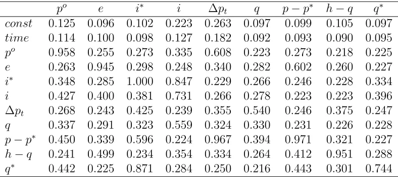
[image:19.595.219.391.465.630.2]Table 4 presents posterior inclusion probabilities for each coefficient in the 11×9 matrix Γ. Of these 99 coefficients, only 13 have posterior inclusion probabilities of greater than 1
2.
9 Often it is the case that the own lag of the
[image:20.595.112.506.268.444.2]dependent variable is the only explanatory variable selected, but there are a few exceptions to this pattern. This reinforces our story that SSVS is an effective method of achieving parsimony in multivariate time series models such as the VECM.
Table 4: Posterior inclusion probabilities for Γ
po e i∗ i ∆p
t q p−p∗ h−q q∗
const 0.125 0.096 0.102 0.223 0.263 0.097 0.099 0.105 0.097 time 0.114 0.100 0.098 0.127 0.182 0.092 0.093 0.090 0.095 po 0.958 0.255 0.273 0.335 0.608 0.223 0.273 0.218 0.225
e 0.263 0.945 0.298 0.248 0.340 0.282 0.602 0.260 0.227 i∗ 0.348 0.285 1.000 0.847 0.229 0.266 0.246 0.228 0.334
i 0.427 0.400 0.381 0.731 0.266 0.278 0.223 0.223 0.396 ∆pt 0.268 0.243 0.425 0.239 0.355 0.540 0.246 0.375 0.247
q 0.337 0.291 0.323 0.559 0.324 0.330 0.231 0.226 0.228 p−p∗ 0.450 0.339 0.596 0.224 0.967 0.394 0.971 0.321 0.227
h−q 0.241 0.499 0.234 0.354 0.334 0.264 0.412 0.951 0.288 q∗ 0.442 0.225 0.871 0.284 0.250 0.216 0.443 0.301 0.744
9
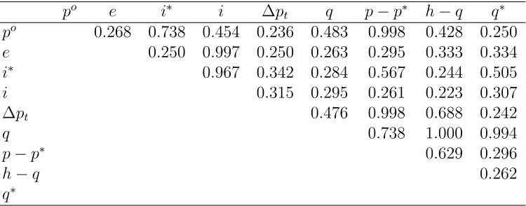
Table 5 also reveals a similar pattern of parsimony. It presents posterior inclusion probabilities for Ψ (which contains the off-diagonal elements of the error covariance matrix). For most of these error covariances the posterior inclusion probability is much less than 1
[image:21.595.120.495.225.372.2]2.
Table 5: Posterior inclusion probabilities for Ψ
po e i∗ i ∆p
t q p−p∗ h−q q∗
po 0.268 0.738 0.454 0.236 0.483 0.998 0.428 0.250
e 0.250 0.997 0.250 0.263 0.295 0.333 0.334 i∗ 0.967 0.342 0.284 0.567 0.244 0.505
i 0.315 0.295 0.261 0.223 0.307
∆pt 0.476 0.998 0.688 0.242
q 0.738 1.000 0.994
p−p∗ 0.629 0.296
h−q 0.262
q∗
3.2
Impulse Response Analysis
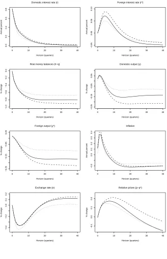
We have seen how SSVS does successfully allow us to work with a very flexi-ble unrestricted model and allow for a more parsimonious restricted model to be picked out automatically. We stress that the alternative strategy of eval-uating every restricted model with a goal to either selecting a single one or doing model averaging is computationally infeasible when facing the number of models that we are dealing with here. Now we present evidence that SSVS is picking out economically-sensible empirical models through a consideration of impulse responses.
Figure 1: Responses to a Monetary Shock. Solid line = SSVS for Everything, Dots = Best Model, Dashes = GLPS model
0 10 20 30 40
0.0
0.2
0.4
0.6
0.8
Domestic interest rate (r)
Horizon (quarters)
Annual percent
0 10 20 30 40
−0.05
0.00
0.05
0.10
Foreign interest rate (r*)
Horizon (quarters)
Annual percent
0 10 20 30 40
−1.0
−0.8
−0.6
−0.4
−0.2
0.0
Real money balances (h−q)
Horizon (quarters)
% change
0 10 20 30 40
−0.25
−0.15
−0.05
0.05
Domestic output (y)
Horizon (quarters)
% change
0 10 20 30 40
−0.25
−0.15
−0.05
0.05
Foreign output (y*)
Horizon (quarters)
% change
0 10 20 30 40
−0.2
0.0
0.1
0.2
0.3
0.4
Inflation
Horizon (quarters)
Annual percent
0 10 20 30 40
−0.4
−0.2
0.0
0.1
0.2
Exchange rate (e)
Horizon (quarters)
% change
0 10 20 30 40
−0.1
0.0
0.1
0.2
Relative prices (p−p*)
Horizon (quarters)
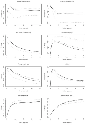
Figure 2: Responses to an Oil Price Shock. Solid line = SSVS for Everything, Dots = Best Model, Dashes = GLPS model
0 10 20 30 40
0.04
0.06
0.08
0.10
Domestic interest rate (r)
Horizon (quarters)
Annual percent
0 10 20 30 40
−0.06
−0.02
0.02
0.06
Foreign interest rate (r*)
Horizon (quarters)
Annual percent
0 10 20 30 40
−0.3
−0.2
−0.1
0.0
0.1
0.2
Real money balances (h−q)
Horizon (quarters)
% change
0 10 20 30 40
−0.05
0.00
0.05
0.10
Domestic output (y)
Horizon (quarters)
% change
0 10 20 30 40
−0.10
−0.06
−0.02
0.02
Foreign output (y*)
Horizon (quarters)
% change
0 10 20 30 40
0.0
0.1
0.2
0.3
0.4
Inflation
Horizon (quarters)
Annual percent
0 10 20 30 40
0.0
0.2
0.4
0.6
0.8
1.0
Exchange rate (e)
Horizon (quarters)
% change
0 10 20 30 40
−0.4
−0.2
0.0
0.2
0.4
0.6
0.8
Relative prices (p−p*)
Horizon (quarters)
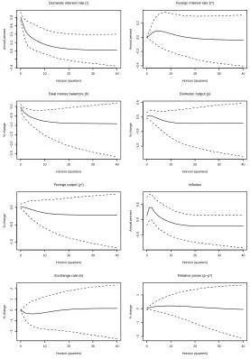
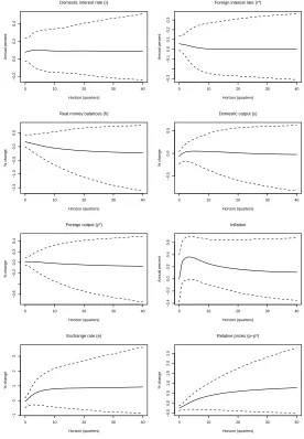
A more detailed set of impulse response functions, including 95% credible intervals, is provided in Appendix D. These credible intervals (similar to the 95% bootstrapped confidence intervals using in Garratt et al, 2003) tend to be fairly wide. Nevertheless, the same pattern of similarity across approaches (and to Garratt et al, 2003) is retained.
4
Conclusions
SSVS methods typically involve, for each parameter, choosing between a tight prior and a loose prior in a data-based fashion. The tight prior is constructed so as to shrink the parameter so that it is effectively zero. In this paper, we have extended these ideas to VECMs and to the case where the researcher is interested in restrictions involving several parameters. These extensions required us to define carefully what a “tight prior” and a “loose prior” was in the case of the cointegration space. An MCMC algorithm was developed for carrying out empirical inference in the resulting model.
References
Chipman, H., George, E. and McCulloch, R. (2001). “The practical im-plementation of Bayesian model selection,” pages 65-134 in Institute of Math-ematical Statistics Lecture Notes - Monograph Series, Volume 38, edited by P. Lahiri.
Doan, T., Litterman, R. and Sims, C. (1984). “Forecasting and condi-tional projection using realistic prior distributions,”Econometric Reviews, 3, 1-100.
Draper, D. (1995). “Assessment and propagation of model uncertainty (with discussion),” Journal of the Royal Statistical Society Series B, 56, 45-98.
Fern´andez, C., Ley, E. and Steel, M. (2001). ”Model uncertainty in cross-country growth regressions,” Journal of Applied Econometrics, 16, 563-576.
Garratt, A., Lee, K., Pesaran, M.H. and Shin, Y. (2003). “A Long-run structural macroeconometric model of the UK economy,”Economic Journal, 113, 412-455
Garratt, A., Lee, K., Pesaran, M.H. and Shin, Y. (2006). Global and Na-tional Macroeconometric Modelling: A Long-Run Structural Approach, Ox-ford: Oxford University Press.
George, E., Sun, D. and Ni, S. (2008). “Bayesian stochastic search for VAR model restrictions,” Journal of Econometrics, 142, 553-580.
Giordani, P. and Kohn, R. (2008). “Efficient Bayesian inference for mul-tiple change-point and mixture innovation models,”Journal of Business and Economic Statistics, 26, 66-77.
Geweke, J. (1996). “Bayesian reduced rank regression in econometrics,”
Journal of Econometrics, 75, 121-146.
Jochmann, M., Koop, G. and Strachan, R. (2009). “Bayesian forecast-ing usforecast-ing stochastic search variable selection in a VAR subject to breaks,” forthcoming in International Journal of Forecasting.
Johansen, S. (1995). Likelihood-Based Inference in Cointegrated Vector Autoregressive Models. Oxford: Oxford University Press.
Koop, Leon-Gonzalez, R. and Strachan, R. (2009a). “Efficient posterior simulation for cointegrated models with priors on the cointegration space,”
Econometric Reviews, forthcoming.
Koop, G., Leon-Gonzalez, R. and Strachan, R. (2009c). “Bayesian in-ference in a cointegrating panel data model,” forthcoming in Advances in Econometrics, volume 23
Koop, G., Potter, S. and Strachan, R. (2008). “Re-examining the con-sumption-wealth relationship: The role of model uncertainty,” Journal of Money, Credit and Banking, 40, 341-367.
Leamer, E. (1978). Specification Searches. New York: Wiley.
Liu, J. and Wu, Y. (1999). “Parameter expansion for data augmenta-tion,” Journal of the American Statistical Association, 94, 1264-1274.
Primiceri. G. (2005). “Time varying structural vector autoregressions and monetary policy,” Review of Economic Studies, 72, 821-852.
Raftery, A., Madigan, D. and Hoeting, J. (1997). ”Bayesian model av-eraging for linear regression models,” Journal of the American Statistical Association, 92, 179-191.
Sala-i-Martin, X., Doppelhoffer, G. and Miller, R. (2004). “Determinants of long-term growth: A Bayesian averaging of classical estimates (BACE) approach,” American Economic Review, 94, 813-835.
Sims, C. and Zha, T. (2006). “Were there regime switches in macroeco-nomic policy?” American Economic Review, 96, 54-81.
Strachan, R. (2003). “Valid Bayesian estimation of the cointegrating error correction model,”Journal of Business and Economic Statistics,21, 185-195. Strachan, R. and Inder, B. (2004). “Bayesian analysis of the error cor-rection model,” Journal of Econometrics, 123, 307-325.
Villani, M. (2005). “Bayesian reference analysis of cointegration,” Econo-metric Theory, 21, 326-357.
Villani, M. (2006). “Bayesian point estimation of the cointegration space,”
Appendix A: Markov Chain Monte Carlo
Al-gorithm
In order to derive the Gibbs sampling algorithm we note that the model can be written as:
Y =Xβ∗α∗+WΓ +E =Zθ+E, E ∼MN(0,Σ, IT), (A1)
where Z ≡(Xβ∗, W) and θ≡(α∗′,Γ′)′. Vectorizing (A1), we obtain:
y= (α∗′⊗X)b∗+ (I
n⊗W)γ+e= (In⊗Z)d+e, e∼N(0,Σ⊗IT), (A2)
where y = vec(Y), a∗ ≡ vec(α∗), b∗ ≡ vec(β∗), γ ≡ vec(Γ), d ≡ vec(θ),
e ≡ vec(E) and Σ = ΨΨ′. We label the nonzero elements of Ψ as ψ ij and
define ψ ≡ (ψ11, . . . , ψnn)′, ηj = (ψ1j, . . . , ψj−1,j)′ and η = (η′2, . . . , η′n)′.
Recall the prior distributions:
a∗|ρ∼N(0, A) with A= diag(ν2 1, . . . , ν
2
nrmax), ν2j = (1−ρj)ν20j+ρjν21j, (A3)
b∗|φ∼N(0, I
rmax ⊗P), (A4)
where P = (HH′ + τ H
⊥H⊥′ ) and φ ∈ {1,2, ..,18} denotes the different
choices for P. Next
γ|δ∼N(0, D) with D= diag(κ2 1, . . . , κ
2
nk), κ2j = (1−δj)κ20j+δjκ21j, (A5)
ψ2jj ∼Gamma(aj, bj), j = 1, . . . , n, (A6)
ηj|ω∼N(0, Fj) withFj = diag(ξ21j, . . . , ξ2j−1,j), j = 2, . . . , n,
ξ2
ij = (1−ωij)ξ20j+ωijξ21j, j = 2, . . . , n, i= 1, . . . , j−1,
(A7)
ρj ∼Bernoulli
pαj, (A8)
δj ∼Bernoulli
pγj, (A9)
ωij ∼Bernoulli
p
ψij
. (A10)
From (A9) and (A10) we can derive the prior distribution for d as
d|ρ, δ∼N(0, G), (A11)
where G is constructed from A and D.
1. b∗ ∼N(¯b,B¯) with
¯
B =(α∗Σ−1
α∗′)⊗(X′X) +I
rmax ⊗P −1−1
(A12)
and
¯b= ¯B(α∗Σ−1⊗X′)[y−(I
n⊗W)γ]. (A13)
2. d∼N( ¯d,D¯) with
¯
D= Σ−1⊗Z′Z+G−1−1 (A14)
and
¯
d= ¯D(Σ−1⊗Z′)y. (A15)
3. ψ2jj are independent of one another ψ2jj ∼Gamma(aj+ 0.5T, bj) with
bj =
(
b1+ 0.5v11, for j = 1, bj + 0.5 [vjj −vj′(Vj−1+Fj−1)−1vj], for j = 2, . . . , n
(A16)
and
V ≡(Y −Xβ∗α∗−WΓ)′(Y −Xβ∗α∗−WΓ) (A17)
has elements vij, vj ≡ (v1j, . . . , vj−1,j)′ and Vj is the upper left j ×j
block of V.
4. ηj are independent of one anotherηj ∼N(ηj, Vj) with
Vj = (Vj−1+Fj−1) (A18)
and
ηj =−ψjjVjvj. (A19)
5. P(φ =φj)∝pj with pj =fN(b∗; 0, Ir⊗Pj) wherefN(.) is the Normal
p.d.f.
6. ρj are independent of one anotherρj ∼Bernoulli(pαj) with
pαj =
1 ν1j
exp
− α 2
j
2ν2 1j
pαj
1 ν1j exp
− α 2
j
2ν2 1j
pαj + 1 ν0j exp
− α 2
j
2ν2 0j
1−pαj
7. δj are independent of one anotherδj ∼Bernoulli(pγj) with
pγj =
1 κ1j
exp
− γ 2
j
2κ2 1j
p
γj
1 κ1j
exp
− γ 2
j
2κ2 1j
p
γj +
1 κ0j
exp
− γ 2
j
2κ2 0j
1−p
γj
. (A21)
8. ωij are independent of one anotherωij ∼Bernoulli(pψij) with
pψij =
1
ξ1ij exp − ψ2ij 2ξ21ij
!
p
ψij
1
ξ1ij exp − ψ2ij 2ξ21ij
!
p
ψij+
1
ξ0ij exp − ψ2ij 2ξ20ij
!
1−p
ψij
.
Appendix B: Further Details on Prior
Elicita-tion
Our SSVS prior for VECMs requires the construction of Hj for j = 1, ..,18
which impose the over-identifying restrictions or restrict the manner in which deterministic trends enters the cointegrating residuals. The manner in which such matrices are constructed is described in Strachan and Inder (2004) and the reader is referred to that paper for details. The matrices below are not semi-orthogonal, but since sp(H) = sp(Hκ) for any full rank square κ, after constructing H, we may innocuously make it semi-orthogonal by the transformation H →H(H′H)−1/2
.
Noting that thetth row ofX is ordered as (1, t, po
t, et, i∗t, it,∆pt, qt, pt−p∗t,
ht−qt, qt∗), the following restriction matrices can be constructed. The matrix
which imposes no restrictions at all and simply leads to the noninformative prior for the cointegrating space defined in the body of the text is:
H1 =I.
The matrix which deletes the deterministic trend term, but otherwise leaves the cointegrating space unrestricted is:
H2 =
1 0 0 0 0 0 0 0 0 0 0 0 0 0 0 0 0 0 0 0 0 1 0 0 0 0 0 0 0 0 0 0 1 0 0 0 0 0 0 0 0 0 0 1 0 0 0 0 0 0 0 0 0 0 1 0 0 0 0 0 0 0 0 0 0 1 0 0 0 0 0 0 0 0 0 0 1 0 0 0 0 0 0 0 0 0 0 1 0 0 0 0 0 0 0 0 0 0 1 0 0 0 0 0 0 0 0 0 0 1
otherwise leaves the cointegrating space unrestricted is:
H3 =
0 0 0 0 0 0 0 0 0 0 0 0 0 0 0 0 0 0 1 0 0 0 0 0 0 0 0 0 1 0 0 0 0 0 0 0 0 0 1 0 0 0 0 0 0 0 0 0 1 0 0 0 0 0 0 0 0 0 1 0 0 0 0 0 0 0 0 0 1 0 0 0 0 0 0 0 0 0 1 0 0 0 0 0 0 0 0 0 1 0 0 0 0 0 0 0 0 0 1
The matrix which imposes the purchasing power parity relationship in (4), but otherwise leaves the cointegrating space unrestricted is:
H4 =
0 1 0 0 0 0 0 0 0 0 0 0 0 0 0 0 0 0 0 0 1 0 0 0 0 0 0
−1 0 0 0 0 0 0 0 0 0 0 0 1 0 0 0 0 0 0 0 0 0 1 0 0 0 0 0 0 0 0 0 1 0 0 0 0 0 0 0 0 0 1 0 0 1 0 0 0 0 0 0 0 0 0 0 0 0 0 0 0 1 0 0 0 0 0 0 0 0 0 1
oth-erwise leaves the cointegrating space unrestricted is:
H5 =
0 1 0 0 0 0 0 0 0 0 0 0 0 0 0 0 0 0 0 0 1 0 0 0 0 0 0 0 0 0 1 0 0 0 0 0
−1 0 0 0 0 0 0 0 0 1 0 0 0 0 0 0 0 0 0 0 0 0 1 0 0 0 0 0 0 0 0 0 1 0 0 0 0 0 0 0 0 0 1 0 0 0 0 0 0 0 0 0 1 0 0 0 0 0 0 0 0 0 1
The matrix which imposes the restriction implied by neoclassical growth models for the UK and the rest of the world in (4), but otherwise leaves the cointegrating space unrestricted is:
H6 =
0 1 0 0 0 0 0 0 0 0 0 0 0 0 0 0 0 0 0 0 1 0 0 0 0 0 0 0 0 0 1 0 0 0 0 0 0 0 0 0 1 0 0 0 0 0 0 0 0 0 1 0 0 0 0 0 0 0 0 0 1 0 0 1 0 0 0 0 0 0 0 0 0 0 0 0 0 0 0 1 0 0 0 0 0 0 0 0 0 1
−1 0 0 0 0 0 0 0 0
is:
H7 =
0 1 0 0 0 0 0 0 0 0 0 0 0 0 0 0 0 0 0 0 1 0 0 0 0 0 0 0 0 0 1 0 0 0 0 0 0 0 0 0 1 0 0 0 0 1 0 0 0 0 0 0 0 0
−1 0 0 0 0 0 0 0 0 0 0 0 0 0 1 0 0 0 0 0 0 0 0 0 1 0 0 0 0 0 0 0 0 0 1 0 0 0 0 0 0 0 0 0 1
The matrix which imposes the first and second of the restrictions in (4) is:
H8 =
0 0 1 0 0 0 0 0 0 0 0 0 0 0 0 0 0 0 0 1 0 0 0 0
−1 0 0 0 0 0 0 0 0 −1 0 0 0 0 0 0 0 1 0 0 0 0 0 0 0 0 0 0 1 0 0 0 0 0 0 0 0 1 0 0 1 0 0 0 0 0 0 0 0 0 0 0 0 0 1 0 0 0 0 0 0 0 0 1
The matrix which imposes the first and third of the restrictions in (4) is:
H9 =
0 0 1 0 0 0 0 0 0 0 0 0 0 0 0 0 0 0 0 1 0 0 0 0
−1 0 0 0 0 0 0 0 0 0 0 0 1 0 0 0 0 0 0 0 0 1 0 0 0 0 0 0 0 0 1 0 0 1 0 0 0 0 0 0 1 0 0 0 0 0 0 0 0 0 0 0 0 0 0 1 0 −1 0 0 0 0 0 0
The matrix which imposes the first and fourth of the restrictions in (4) is:
H10 =
0 0 1 0 0 0 0 0 0 0 0 0 0 0 0 0 0 0 0 1 0 0 0 0
−1 0 0 0 0 0 0 0 0 0 0 0 1 0 0 0 0 1 0 0 0 0 0 0 0 −1 0 0 0 0 0 0 0 0 0 0 0 1 0 0 1 0 0 0 0 0 0 0 0 0 0 0 0 0 1 0 0 0 0 0 0 0 0 1
The matrix which imposes the second and third of the restrictions in (4) is:
H11 =
0 0 1 0 0 0 0 0 0 0 0 0 0 0 0 0 0 0 0 1 0 0 0 0 0 0 0 0 1 0 0 0
−1 0 0 0 0 0 0 0 1 0 0 0 0 0 0 0 0 0 0 0 0 1 0 0 0 1 0 0 0 0 0 0 0 0 0 0 0 0 1 0 0 0 0 0 0 0 0 1 0 −1 0 0 0 0 0 0
The matrix which imposes the second and fourth of the restrictions in (4) is:
H12=
0 0 1 0 0 0 0 0 0 0 0 0 0 0 0 0 0 0 0 0 0 1 0 0 0 0 0 0 0 0 0 1 0 0 0 0
−1 0 0 0 0 0 0 0 0 1 1 0 0 0 0 0 0 0 0 −1 0 0 0 0 0 0 0 0 0 0 0 0 1 0 0 0 0 0 0 0 0 0 1 0 0 0 0 0 0 0 0 0 1 0 0 0 0 0 0 0 0 0 1
The matrix which imposes the third and fourth of the restrictions in (4) is:
H13 =
0 0 1 0 0 0 0 0 0 0 0 0 0 0 0 0 0 0 0 1 0 0 0 0 0 0 0 0 1 0 0 0 0 0 0 0 0 1 0 0 0 1 0 0 0 0 0 0 0 −1 0 0 0 0 0 0 1 0 0 0 0 0 0 0 0 0 0 0 0 0 1 0 0 0 0 0 0 0 0 1
−1 0 0 0 0 0 0 0
The matrix which imposes the first, second and third of the restrictions in (4) is:
H14 =
0 0 0 1 0 0 0 0 0 0 0 0 0 0 0 0 0 0 1 0 0
−1 0 0 0 0 0 0 0 −1 0 0 0 0 0 0 1 0 0 0 0 0 0 0 0 0 0 1 0 0 0 1 0 0 0 0 1 0 0 0 0 0 0 0 0 0 0 0 0 1 0 0 −1 0 0 0 0
(4) is:
H15 =
0 0 0 1 0 0 0 0 0 0 0 0 0 0 0 0 0 0 0 0 1 0 0 0
−1 0 0 0 0 0 0 0 0 −1 0 0 0 0 0 0 0 1 1 0 0 0 0 0 0 0 −1 0 0 0 0 0 0 0 0 0 0 1 0 0 1 0 0 0 0 0 0 0 0 0 0 0 0 0 1 0 0 0 0 0 0 0 0 1
The matrix which imposes the first, third and fourth of the restrictions in (4) is:
H16 =
0 0 0 1 0 0 0 0 0 0 0 0 0 0 0 0 0 0 1 0 0
−1 0 0 0 0 0 0 0 0 0 0 0 1 0 0 0 1 0 0 0 0 0 0 −1 0 0 0 0 0 1 0 0 0 0 0 1 0 0 0 0 0 0 0 0 0 0 0 0 1 0 −1 0 0 0 0 0
(4) is:
H17 =
0 0 0 1 0 0 0 0 0 0 0 0 0 0 0 0 0 0 0 0 1 0 0 0 0 0 0 0 0 1 0 0
−1 0 0 0 0 0 0 0 1 0 1 0 0 0 0 0 0 0 −1 0 0 0 0 0 0 1 0 0 0 0 0 0 0 0 0 0 0 0 1 0 0 0 0 0 0 0 0 1 0 −1 0 0 0 0 0 0
The matrix which imposes all of the restrictions in (4) is:
H18 =
0 0 0 0 1 0 0 0 0 0 0 0 0 0 0 0 0 0 0 1 0
−1 0 0 0 0 0 0 0 −1 0 0 0 0 0 0 1 0 1 0 0 0 0 0 0 −1 0 0 0 0 0 1 0 0 0 0 1 0 0 0 0 0 0 0 0 0 0 0 0 1 0 0 −1 0 0 0 0
Appendix C: Data Appendix
The data set is an updated version of the data set constructed by Garratt et al. (2003) and runs from 1965Q1 through 2008Q1. The variables are:
1. qt: the natural logarithm of UK real per capita domestic output,
com-puted as:
ln(GDPt/P OPt).
GDPt is real gross domestic product (at 1995 prices; 1995=100;
sea-sonally adjusted; source: Office of National Statistics (ONS), Economic Trends, code: YBEZ). P OPt is total UK population (in thousands;
source: ONS, Monthly Digest of Statistics, code: DYAY, annual se-ries), which was available up to 2007. The 2008 number is obtained by extrapolating the 2007 number using the average growth rate for the period 2003-2007. The population series is converted into a quarterly series through geometric interpolation and rebased 1995=1.
2. pt: the natural logarithm of the domestic price level, computed as:
ln(Pt),
where Pt is the UK producer price index (manufactured products;
1995=100; not seasonally adjusted; source: ONS, Economic Trends, code: PLLU).
3. ∆pt: the UK inflation rate, computed as:
ln( ˜Pt)−ln( ˜Pt−1),
where ˜Ptis the UK retail price index (all items; 1995=100; not
season-ally adjusted; source: ONS, Economic Trends, code: CHAW).
4. it: the quarterly domestic nominal interest rate, computed as:
1 4ln
1 + Rt 100
×100,
where Rt is the 90 day treasury bill average discount rate (annualized
5. ht − qt: the natural logarithm of real per capita money stock as a
proportion of real per capita income, computed as:
ln
Ht
Yt
,
whereHtis the M0 money stock (end period; in Million Pound Sterling;
seasonally adjusted; source: ONS, Financial Statistics, code AVAE). The AVAE series was available for the period 1969Q2-2006Q1. Out-side this period the series is projected using the percentage change of estimated circulation of notes and coins with the public. Nominal in-come Yt is measured using gross domestic product at market prices (in
Million Pound Sterling; seasonally adjusted, source: ONS, Economic Trends, code: YBHA).
6. et: the natural logarithm of the UK nominal effective exchange rate,
computed as:
−ln(Et),
where Et is the Sterling effective exchange rate (1995=100; source:
ONS, Financial Statistics, code: AGBG (old code: AJHX); ONS de-finesEtas the foreign price of domestic currency, hence the minus sign).
The AGBG series was available until 2006Q1. Afterwards, we project the series using the percentage change of a broader exchange rate index (source: ONS, Financial Statistics, code: BK82).
7. q∗
t: the natural logarithm of real per capita foreign output, computed
as:
ln
GDP∗ t
P OP∗ t
,
whereGDP∗
t is the gross domestic product index for the original OECD
countries (at 2000 prices; 1995=100; seasonally adjusted; source: OECD, Main Economic Indicators (MEI), code: OTF.VPVOBARSA.2000.S1). P OPtis the population of these countries (annual series; source: OECD,
8. p∗
t: the natural logarithm of the foreign price index, computed as:
ln(P∗ t),
whereP∗
t is the OECD producer price index (1995=100; source: OECD,
MEI, code: OTO.PPI). Data was available on this series from 1982Q1. The data prior to 1982Q1 was constructed by backwardly imposing the percentage changes of a separately constructed weighted average index of OECD consumer and producer prices on the 1982Q1 figure.
9. i∗
t: the quarterly foreign nominal interest rate:
1 4ln
1 + R
∗ t
100
×100,
with R∗
t being a weighted average of foreign annualized interest rates
computed as:
R∗
t = 0.4382R
US
t + 0.236R
Germany
t + 0.2022R
Japan
t + 0.1236RFrancet .
The weights are chosen according to Garratt et al. (2003). The an-nualized interest rates are all from the IMF’s International Financial Statistics (IFS). For the US we use the three-month treasury bill rate (code: 60C.ZF), for Germany the money market rate (code: 60B.ZF), for Japan the money market rate (code: 60B.ZF) and for France the three-month treasury bill rate (code: 60C.ZF).
10. po
t: the natural logarithm of the oil price, computed as:
ln(Pto),
where Po
t is the average price of crude petroleum (in US dollar per
Appendix D: Additional Empirical Results
[image:42.595.162.442.258.661.2]In the text, point estimates of the impulse responses were provided (these remain the solid lines in the figures below). Here we also add 95% credible intervals (the dashed lines in the figures below) to give the reader some idea of the dispersion associated with the point estimates.
Figure D1: Response to a Monetary Shock (SSVS for Everything)
0 10 20 30 40
−0.4
0.0
0.2
0.4
0.6
0.8
Domestic interest rate (r)
Horizon (quarters)
Annual percent
0 10 20 30 40
−0.4
−0.2
0.0
0.2
Foreign interest rate (r*)
Horizon (quarters)
Annual percent
0 10 20 30 40
−2.5
−2.0
−1.5
−1.0
−0.5
0.0
Real money balances (h)
Horizon (quarters)
% change
0 10 20 30 40
−1.0
−0.5
0.0
0.5
Domestic output (y)
Horizon (quarters)
% change
0 10 20 30 40
−1.0
−0.6
−0.2
0.2
0.4
Foreign output (y*)
Horizon (quarters)
% change
0 10 20 30 40
−0.5
0.0
0.5
Inflation
Horizon (quarters)
Annual percent
0 10 20 30 40
−2
−1
0
1
2
Exchange rate (e)
Horizon (quarters)
% change
0 10 20 30 40
−2
−1
0
1
Relative prices (p−p*)
Horizon (quarters)
Figure D2: Response to a Monetary Shock (Best Model)
0 10 20 30 40
−0.2
0.0
0.2
0.4
0.6
0.8
Domestic interest rate (r)
Horizon (quarters)
Annual percent
0 10 20 30 40
−0.3
−0.2
−0.1
0.0
0.1
0.2
Foreign interest rate (r*)
Horizon (quarters)
Annual percent
0 10 20 30 40
−2.0
−1.5
−1.0
−0.5
0.0
Real money balances (h)
Horizon (quarters)
% change
0 10 20 30 40
−0.8
−0.4
0.0
0.2
0.4
Domestic output (y)
Horizon (quarters)
% change
0 10 20 30 40
−0.8
−0.6
−0.4
−0.2
0.0
0.2
0.4
Foreign output (y*)
Horizon (quarters)
% change
0 10 20 30 40
−0.6
−0.2
0.2
0.4
0.6
Inflation
Horizon (quarters)
Annual percent
0 10 20 30 40
−2
−1
0
1
Exchange rate (e)
Horizon (quarters)
% change
0 10 20 30 40
−1.5
−1.0
−0.5
0.0
0.5
1.0
Relative prices (p−p*)
Horizon (quarters)
Figure D3: Response to a Monetary Shock (GLPS Model)
0 10 20 30 40
−0.4
0.0
0.2
0.4
0.6
0.8
Domestic interest rate (r)
Horizon (quarters)
Annual percent
0 10 20 30 40
−0.4
−0.2
0.0
0.2
Foreign interest rate (r*)
Horizon (quarters)
Annual percent
0 10 20 30 40
−2.5
−2.0
−1.5
−1.0
−0.5
0.0
Real money balances (h)
Horizon (quarters)
% change
0 10 20 30 40
−1.0
−0.5
0.0
0.5
Domestic output (y)
Horizon (quarters)
% change
0 10 20 30 40
−1.0
−0.5
0.0
Foreign output (y*)
Horizon (quarters)
% change
0 10 20 30 40
−0.5
0.0
0.5
Inflation
Horizon (quarters)
Annual percent
0 10 20 30 40
−2
−1
0
1
2
Exchange rate (e)
Horizon (quarters)
% change
0 10 20 30 40
−2
−1
0
1
Relative prices (p−p*)
Horizon (quarters)