Software reliability prediction

City, University of London Institutional Repository

Citation

:

Chan, Pee Yuaw (1986). Software reliability prediction. (Unpublished Doctoral thesis, The City University London)

This is the accepted version of the paper.

This version of the publication may differ from the final published

version.

Permanent repository link:

http://openaccess.city.ac.uk/18127/

Link to published version

:

Copyright and reuse:

City Research Online aims to make research

outputs of City, University of London available to a wider audience.

Copyright and Moral Rights remain with the author(s) and/or copyright

holders. URLs from City Research Online may be freely distributed and

linked to.

Pee Yuaw CHAN

Thesis Submitted for

the Degree of Doctor of Philosophy in Statistics and Computer Science

DEPARTMENT OF MATHEMATICS

THE CITY UNIVERSITY

LONDON

West Yorkshire, LS23 7BQ www.bl.uk

BEST COpy AVAILABLE.

West Yorkshire, lS23 7BQ www.bl,uk

DAMAGED

my moods and absent-minded ness

for the past one and a half years,

and had to spend two months

on her own during the preparation

CONTENTS

ACKNOWLEDGEMENTS

ABSTRACT

KEY TO ABBREVIATIONS

CHAPTER 1. INTRODUCTION

CHAPTER 2. TWO METHODS FOR UNCONSTRAINED MINIMISATION

2.1. Introduction

2.2. The need of an efficient algorithm for parameter estimation

2.3. The univariate method

2.4. The multi-variate minimisation method

CHAPTER 3. IMPLEMENTATION OF THE MINIMISATION METHODS

AND NUMERICAL RESULTS

3.1. Introduction

3.2. The Jelinski

&

Moranda system (3M)

3.3. The Bayesian Jelinski

&

Moranda system

3.4. The Geol and Okumoto system (00)

3.5. The Musa and Okumoto system (Me»

3.6. The Duane system (DU)

3.7. The Littlewood system (L)

3.8. The Littlewood NHPP system (LNHPP)

3.9. The Littlewood and Verrall syst_ (LV)

3.10.The Keiller and Littlewood system (KL)

3. 11. Implementation and modifications

3.12.Numerical results

(8JM)

CHAPTER 4.

CHAPTER 5.

MEASUREMENT AND ANALYSIS OF THE PREDICTIVE QUALITY

OF ORDINARY AND ADAPTIVE PREDICTION SYSTEMS

4.1. Introduction

4.2. Measuring predictive quality

4.2.1.

4.2.2.

4.2.3.

4.2.4.

The u-plot procedure

The y-plot procedure

The prequential likelihood

Median plots

4.2.5. Summary

4.3. The u-plot and adaptive modelling

4.4. The analysis of predictive quality of

adaptive prediction systems

THE DETERMINATION OF THE PARAMETRIC SPLINE ADAPTOR

AND THE ANALYSIS OF THE RESULTS OF THEIR APPLICATION

5.1. Introduction

5.2. The smooth adaptive curve

5.3. The redundant representation and the least

-squares solution of the constrained

70 71 73 74 75 82 82 82 86 102 103

cubic spline 107

5.4. The B-spline representation of the cubic

spline 113

5.5.

Method for the determination of the

over-constrained cubic spline 119

5.6. Quality of the predictions by parametric

CHAPTER 6.

CHAPTER 7.

APPENDIX 1.

APPENDIX 2.

APPENDIX 3.

APPENDIX 4.

SOFTWARE RELIABILITY PREDICTION SYSTEMS WITH

NON-PARAMETRIC RATE ESTIMATES AND THE ANALYSIS

OF THEIR PERFORMANCE.

6.1. Introduction 159

6.2. Estimation of the completely monotone rates 160

6.3. Prediction systems with monotone rate estimates 163

6.4. Analysis of the quality of the predictions

using monotone rate estimates

SlM-iARY AND CONCLUSIONS AND FUTURE RESEARCH

POSSIBILITIES

7.1. Summary and Conclusions

7.2. Future research possibilities

164

179

183

Uniqueness and condition for finite maximum likelihood

parameter estimate in the Gael and Okumoto model. 186

A non-parametric approach to estimate the failure

rates of a program undergoing debugging.

Listing of the software reliability data.

Median Plots

191

196

204

ACKNOWLEDGEMENTS

This research was done while I was a research assislant at the Cent.re

for Software Reliability, the City University, London. I would like to express my gratitude to:

Professor B. Littlewood for his supervision.

ICL pIc for financing the research project.

numerous slaff members of the Mathematics Department and the

Computer Science Department at The City University, in particular

Mr.J.Snell for his involvement and assistance.

Dr.M.G.Cox at the National Physical Laboratory (NPL) for his valuable

advice, and the Publications Officer at NPL for supplying me with a

number of useful report.s.

Professor D.R. Miller and Dr.A. Sofer for the use of their software.

t.he slaff of t.he Computer Unit at. City University.

Ms.G. Palmer for typing the title of the graphs and plots in the thesis.

Mrs.D. Carmen for her efficient and skillful typing of this thesis, and

her patience in making numerous changes from the draft version to its present form.

my parents, brother, sisters, and my wife for their understanding and

support.

Mr. and Mrs.P. Man for their help back in 1976 which made all this

ABSTRACT

Two methods are proposed to find the maximum likelihood parameter estimates of a number of software reliability models. On the basis of the results from analysing 7 sets of real data, these methods are found to be both efficient and reliable.

The simple approach of adapting software reliability predictions by Keiller and Littlewood (1984) can produce improved predictions, but at the same time, introduces a lot of internal noise into the adapted predictions. This is due to the fact that the adaptor is a joined-up function.

An alternative adaptive procedure, which involves the parametric spline adaptor, can produce at least as Jtood adapted without the predictions being contaminated by internal noise simple approach.

use of a predictions

as in the

Miller and Sofer (1986a) proposed a method for estimating the failure

rate of a program non-parametrically. Here, these non-parametric rates

KEY TO

ABBREVIATIQ~S

BJM( *)

cdf

dDIF(*)

DU( *)

GO( *)

GP

HPP

JM( *)

KL( *)

KS

L(*)

LNHPP(*)

LV( *)

ML MLE MNA MO(*) NHPP pdf PL PLR ROCOF SQAMA w.r.t.

The (adapted) Bayesian Jelinski and Moranda prediction system

Cumulative distribution function

The (adapted) prediction system with exponential failure time and monotone rate estimates with d difference constraints

The (adapted) Duane prediction system

The (adapted) Goel and Okumoto prediction system

The generalised power law NHPP prediction system

Homogeneous Poisson process

The (adapted) Jelinski and Moranda prediction system

The (adapted) Keiller and Littlewood prediction system

Kolmogorov and Smirnov

The (adapted) Littlewood prediction system

The (adapted) Littlewood NHPP prediction system

The (adapted) Littlewood and Verrall prediction system

Maximum likelihood

Maximum likelihood estimate

Modified Newton's algorithm

The (adapted) Musa and Okumoto prediction system

Non-homogeneous Poisson process

Probability density function

Prequential likelihood

Prequential likelihood ratio

Rate of occurrence of failures

The safeguarded quadratic approxiaation aini.isation algorithm

CHAPTER 1

INTRODUCTION

Complex sottware sY8tem8 contain desiarn error8 which mayor may not manife8t them8elve8 by cau8ing failures durin" execution. A failure occur8 when there i8 a di8crepancy between the output of the program and ita specification. When this happens, an attempt will usually be made to identify the 80urce of the failure and remove it. This process of debuarging, if succes8ful, would lead to an improvement in the reliability of the pro"ram. The main objective

ot

this work is to measure the reliability of 80ft ware system8 underaroinar debuar"nar. This would be of interest to a software developer who want8 to know whether a pro"ram is reliable enouarh for marketinar or more development effort is needed before reachin" that sta"e. It i8 al80 of interest to a user who wants to know whether the reliability of a proarram has reached the level required for hi8 particular application. This is of particular importance if the software would be u8ed to control or monitor system8 where an operational failure would have

disastrou8 consequences.

Software reliability evaluation methodoloaies developed up to the

present are built on the foundation t.hat t.he underlyina proces8 aovernina the failure behaviour of a soft.ware is random. An account. for t.he

randomness in software failure. i. ariven by Laprie (1984). While software

reliability modellera miarht disaaree on t.he sources of such randomnes.,

there i. ,eneral acceptance t.hat t.he reliability of a pro,ram can only be

commonly used is for the operational reliability of a pro.ram. which is the probability of successful execution of the program without failure for a specified len.th of time in a specified environment.

Here we will concentrate on data of the form tl .tz'."'~ of execution times between successive failures of a pro_ram under.oin. debu •• in •• and methods which utilise this information to predict the unobserved random

quantities Ti+l'Ti+z.... • estimating the current

In particular, we focus our attention on reliability, i.e. characteristics of the random variables Ti+l; other unobserved quantities can be dealt with in a similar way. Note that this estimation problem is one

ot

prediction because it concerns the unobaerved quantity Ti+l. In principle, what we need ia the probability distribution of the random variable Ti+l' and the problem ia effectively solved if we can accurately eaUmate this diatribution.

In order

to

achieve the above objective, a prediction ayatem bas

to

be uaed. Such a ayatem will allow us

to

predict the future (Ti+l) from the paat

(ts

,tz ...

t.t).

It conaiata of the followin.:

1. A mathematical model detailin. tbe behaviour

ot

the random variable (T_{1,Tz , ... ,Ti) for all i, conditional on IIOme unknown} parametera.

2. A atatiatical interence procedure tor eaUmatin, tbese unknown parametera uain. observed data.

3. A prediction procedure combinin. (1) and (2)

to

allow ua

to

A 8urvey by Dale and Harris (1981) has shown that there are now more than 40 software reliability model8 in exi8tence. Many such model8 with a particular choice of (2) and (3) forms a prediction 8Y8tem which could be

used for the purpo8e of reliability mea8urement.

However, not merely do we want to have a probabilistic profile of the unobserved time to failure, we want one which i8 close to reality. In order to achieve this, it is e8sential to have a ,ood model (1) in the prediction syst.em and at the same time, parts (2) and (3) are also of vital importance. Viewed from this antle, the usual discussion of competint 8Oft.ware reliability models becomes inadequate. We should, instead, be comparing the relative merits of different prediction systems rather than just. the model alone: the auccess or failure of a prediction system is a result of (1), (2) and (3) jointly.

As far a8 selectint a model is concerned, it is not possible to decide, a priori, the best model in any ,iven context. Althou,h one miMht ar,ue

that some models are more suitable because of their realistic assumption8, this still leaves us those which we cannot reject on the ,rounds of bein. unreali8tic. Indeed, the knowled,e in t.his . . pect of software en,ineerint

is so imperfect that it is not possible

to

identity the best model ,iven all t.he characteristica of t.he 80ftware concerned. Our approach is

to

employ many prediction systema simultaneously and

to

aelect t.he best prediction on the basis of the paat predictive quality of each individual 8Y8tem on t.he

A common characterstic shared by the majority of 80ftware reliability models is that it is very hard to carry out a full Bayesian analysis on the unknown paramet.ers. The method of maximum likelihood is usually used in part (2). By this method, a set

ot

parameter values has to be determined such that the likelihood function ia maximised. In practice, this constitutes the bulk of the numerical work that haa to be done in the whole prediction process. The amount of work involved varies trom model to model. In a few cases, it is small because the problem is straight-forward and can be 80lved easUy, but in t.he remaining cases, it. is considerable because the maximisation is by no means t.rivial and can only be done by numerical search. With our multi-prediction systems approach, in particular, the requirement on computing re80urces can be a problem. In view of this, t.here is a definite need to develop efficient

numerical algorithms in order to save computing time.

Chapter 2 describes two numerical algorit.hms tor unconstrained optimisation. These methods are chosen lor t.heir efficiency and well proven success with many practical problems.

Chapter 3 outlines the actual implementation of t.hese al,corithms to 7 of t.he 9 80ftware reliability models included in thil Itudy. Difficulties encountered in analysing real data . t s make it necelaary

to

refine thele algorithms. Full details of t.he numerical experience in analysing 7 real

Having obtained the parameter estimates, the respective prediction systems can proceed to predict. Our next step is to analyse the predictive quality of each of these prediction systems. In Chapter 4 we

present the tools that would be used to evaluate t.he predictive performance, namely, the u- and y-plot procedures, the prequential likelihood, and the median plot.

An important by-product of our analysis of predictive quality is that the u-plot can be used to recalibrate our future predictions. Keiller and Littlewood (1984) have reported acme auccess, on the basis of the u-plot and y-plot criteria when they adapt future predictiona by joinin. up the u-plot and use it aa the calibration curve. However, when we invesU,ate further uain. prequential likelihood aa the criterion of aucceas, the adapted predictionl are not always an improvement. The di . . . reement with the other criteria ateml from the fact that the adapUve curve il a joined-up function, and it can be resolved by usin, a amooth funcUon

instead.

The amooth function we have uaed ia a ~metric apline. In Chapter 5, the parametric spline is defined in terms of B-aplinea, and a numerically atable and efficient method for ita determination ia described. Extenaive

analYles are also ,iven when we apply this method of adapUn, to 9 models and 7 eets of data.

One of the atron,eat criticiams of software reliability modela ia that

non-parametric approach to estimate the failure rate of a program. In

Chapter 6 we shall analyse the quality of the predictions based on rates

estimated by this non-parametric method and exponential failure time

distribution. These predictions are adapted usin~ our parametric spline

adaptor and we compare all the re8ults including those in Chapter 5. An

alternative non-parametric rate e8timation procedure is ~iven in Appendix

2.

The final Chapter is devoted to discussions and future research

CHAPTER 2

TWO METHODS FOR UNCONSTRAINED MINIMISATION

2.1.

INTRODUCTION

In this Chapter we shall describe two numerical optimisation methods for the efficient determination of the maximum likelihood estimate

(MLE)

of the unknown parameters in the software reliability models included in this study. Both methods are for unconstrained optimisation. The first is for optimising functions in one variable. This method, which is due to Gill and

Murray (1974), uses the value of the objective function only. The second

is for functions in more than one variable and is also due

to

Gill and Murray (1972a, 1972b); extensive result.s on BOIvin, man, telt functions and an Algol implementation can be found in the cited publicat.ions. Unlike the univariate optimisation met.hod, the latter requires both t.he gradient. and the value of t.he objective function. This is because the multivariate problems are more difficult., at least in the cases considered here. Wit.h the ext.ra gradient. information the problem can be solved much more efficiently.

The implementation details of t.hese techniques are in Chapter 3.

2.2. THE NEED OF AN BFFIOIBNT ALGORITHM FOR PAJW(BTBR BSTIMATION

Alt.hou,h all t.he three componentl in a prediction 1,Item are important

to the prediction process as a whole, the attention

.0

far bein, ,iven

to

various aspects concernin, the related problem in the .taUIUcal interence

mi,ht ,ive the imprellion that it is ulually' .imple and It.rai,ht-forward.

We believe that a user of any software reliability models should adopt. a Bayesian inference procedure. This involves updat.in, the prior distribution, via the likelihood of the data, to arrive at. the posterior distribution of the parameters. This poat.erior diatribution is then uaed to ,enerate a predictive diat.ribution. A ,ood account of this approach in the context of conventional atatiatical problema i& ,iven in the book by Aitchison and Dunsmore (1975).

In practice, it is often not possible to carry out a full Bayeaian analysis with moat models and the method of maximum likelihood (ML) ia commonly uaed instead. When the maximum of the likelihood function cannot be found analytically, aa ia usually the caae, numerical optimiaation technique has to be employed. The sequential nature in which the inference has to be repeated means that the requirement on computer time can be subatantial, if an inefficient numerical al.orithm ia bein, uaed. Thia would be compounded if one were

to

uae many prediction aystems simultaneously in order to select the most appropriate one.

With the advancement of micro-computer technolo,y, it ia now poaaible for a personal computer to carry out mathematical calculations wit.h accuracy comparable to that of a mainframe computer. Therefore, a atep towards alleviatin, the computer resource problem ia to implement t.he analysis pro,ram on a personal computer. Thia ia obvioualy much more affordable even if t.he personal computer baa to be dedicated ent.irely tor

were to carry out a simulation study on the performance of aeveral prediction ayatema, the waatage in uaing an inefficient method will preclude

the analyaia of more replica tea.

Hencefort.h, we shall only addreaa the problem of minimiaation. The equivalent. maximisation problem merely involvea a change of aign in the objective function. f(x) will be uaed to denote the objective evaluated at x. The variable x ia either a acalar or a vector depending on whether the problem ia univariate or multi-variate. In the latter, ,(x) ia uaed to denote the vector of partial derivativea of the objective and G(x) denotea the Heaaian matrix.

2.3. THE UNIVARIATE MINIMISATION METHOD

Thia ia a hybrid technique which combines two univariate minimisation methods, succeaaive quadratic approximation and function-comparison, in auch a way that it ia haa the apeed of the former and the reliability of the latter. Like moat univariate minimisation method., it utilises the concept of an intervauf uncertainty, i.e. an interval [a,b], which while the minimum is known to lie within it, we are uncertain

a.

to where exactly it ia. The value of auch an interval derive. from the fact that any esUmate lying within it will not be more than the len,th of the interval away from the true minimum. If the function i. unimodal this minimum is ,lobal

Given an initial interval of uncertainty, different methods adopt different atrate.ries to pro.rreasively reduce the aize of this interval until it is sufficiently amall. To illuatrate how this ia done iteratively, we .rive an example where only function valuea are involved. Let [a, b) be the current interval of uncertainty, x is the best point yet, w the previous x value and v is the hi.rhest point of the three. The labellin.r of wand v bas no ai.rnificance here but it. would be necessary to do ao in the method we propose. Fi.rure 2.1. ahows how they are confi.rurated.

v

a x

Fiaure 2.1.

w b

A univariate minimisation alaorit.hm will t.hen predict a point uc[a.b] at. which the objective will be evaluated. How u ia determined will depend on

the method beina uaed. It thia ia u, and f(u,) ia hi,her t.han f(x), t.hen t.he lower bound, a, ia moved

to

point u,. If t.hia point ia Uz and f(uz) i.

next iteration. and the length of the interval is reduced while the minimum remains bracketed.

Popular function-comparison methods like the Fibonacci 8ftarch and the Golden Section search (see Jacoby et aI, 1972, or most introductory textbooks on numerical optimisation for further details of these methods) are reliable, but because t.hey do not lake into consideration the quantity by which the objective chan.es within the interval, t.hey are inefficient. To overcome this, methods based on successive polynomial approximation were developed. This claaa of methods involves repeated fiUin. of polynomials to approximate the function and to use the minimum of the fitted curve to predict the minimum of the objective. In the case where only function values are available, a quadratic function is used. When the ,radient ia alao available, a cubic function i. used instead.

The stationary point of a quadratic pas.in, throu,h the points (x,f(x», (w,f(w)) and (v,f(v)) is ,iven by x + p/q where:

p

=

*

[(w-x)Z(f(v)-f(x» - (v-x)Z(f(w)-f(x»] (2.3.1a)

q

= •

2[(v-x)(f(w)-f(x» - (w-x)(f(v)-I(x»] (2.3.1b)

The equation of the .lope of a cubic passin, throu,h the pointe (x,f(x», (w,f(w» with derivatives f'(x) and f'(w) respectively, is .iven b1:

where

The root of f leu)

=

0 corresponding to a minimum of the fitt.ed cubic can be expressed as x + p/q, where:

p

=

:l: (w - x) [f' (x) - Y - 1'\1 (2.3.2a)

q

=

~[f' (w ) - f' (x) + 2y] (2.3.2b)

with

y

=

sign(w - x)[1'\2 - f' (x)f '(w)

'14

(2.3.2c)

These formulae are commonly available in the literature on numerical optimisation.

With a ,ood starting point, this method can be very efficient, especially when it is near the minimum and the objective is well approximated by a quadratic or cubic. However, if the startin, value ts not sufficiently close to the minimum, it can be unreliable. The common situation causin, difficulty is when one of the function values uaed for the curve fitUn, is very lar,e compared to the rest. On applyin, (2.3.1) or (2.3.2), the predicted minimum will tend to be very close to t.he amall value. Since

only, the larae value will be retained for a while before it ia bein. di8carded, thu8 810win, down the aearch con8iderably. Indeed, a natural

alternative ia to diacard the hiah point since it is likely to be the least

useful in future approximations. Unfortunately, the new point8 which

re8ult will not nece8sarily bracket t.he minimum and in t.his situation t.he

predicted minimum uBina (2.3.1) or (2.3.2) cannot be t.ru8ted, becau8e it is

bein, extrapolated.

The diBadvantaaea of theae methods when used alone can be effectively

eliminated by cambinina them toaether. We will focu8 our attention on

The ba8ic st.rateay here i8 to retain

the lowest function value8 obtained 80 far for fUtina the quadratic, and

when we are in an extrapolaUna position, a bound i8 set up to ufe,uard

the reliability of the predicted minimum.

Fi.ure 2.2. is a typical situation in practice wit.h (atb] bein, the

current. int.erval of uncertainty. The minimum point predicted by the

quadratic throu,h x, wand v will be obviou8ly unreliable because it is

f(v)

d --+1+4

- - + - -__

2

1

v w

x

m

extrapola ting. A possible aafeguard is to build an artificial bound m within the interval [a,b] such that the predicted point cannot exceed m. The artificial bound being used here is defined as follows:

where

and

or

/l(a - x)

m

=

_{

X +

x + /lCb - x)

fJ::::

!UC-d

1 /d2

)U

5/ 11CO.1 - d2/d1 )

d₂

=

b - x

d_z

=

a - x

}

}

if w

>

x if w

<

x

if

Idd<ld21

if

Idd)ld21

if w

<

x

if

w

>

x

(2.3.38)

(2.3.3b)

(2.3.3c)

step defined by (2.3.3) will be referred to as a compari80n step becau8e one can devi8e a univariate function-comparison minimisation al&,orithm using (2.3.3) only.

The tolerance for the purpo8e of terminating the search i8 a function of the relative error C' and the absolute error T. This function is defined

as:

tol(x) : C'lxl + T

and the al,orithm is said to have conver,ed to the minimum if max (x-a.b-x)

<.

2tol(x). The two scalars C' and T will depend on the accuracy of the

computer bein, used. A suitable choice is to set C' and T to ~t/z when

the computation is carried out on a computer with t-bit wordlen,th.

With practical problems, we are often '-norant even about the approximate location of the minimum. If we were to specify an interval of uncertainty throu,h &,uessin" this would most certainly lead to an overstatement of the initial interval 80 that we can be sure that it brackets

the minimum. In our pro,ram, we set t.he init.ial step-size to be O.llxl+lOOtol(x), where x is t.he startin, value. This step is t.hen taken. If the new point is hi,her t.han t.he startin, point t.hen all subsequent step a will be taken in t.he opposite direction. ot.herwise we will continue to take positive steps. The size of each subsequent step ... 4 tilDe. the previous step. The lower (if positive step) or upper (it ne,aUve step)

continues until a higher point is located in which case we have bracketed the minimum and the safeguarded quadratic minimisation algorithm is used to shrink this interval until it satisfies the termination condition.

Because of rounding error in the computation of f(x), apurious modes can be int.roduced even if they are not. present in the function. This can be dealt with by prohibiting the evaluation of the objective at points which are less than some amall diatance apart.. In algorithmic terms, this means we have to make sure that the predicted point ia at leaat a diBtance of tol(x) away from x, a and b. This iB the reason why in definition (2.3.3) the aituation of w

=

x iB excluded. However, there is a need to modify (2.3.3c) Blightly. Since the point predicted by a comparison step ia alwaYB in d_{2 ,} therefore, if d₂

<.

tol(x) we must interchange d_{1 and dz , and the} larger half of the interval can then be reduced rapidly.

If we merely keep the predicted point a distance of tol(x) from points x, wand v, thiB could lead to many ateps of aize tol(x) being taken. A8 a precaution against this, a comparison atep i8 laken whenever lei

<.

tol(x),

where e ia the st.ep taken in the laat-but-one iteration. A comparison atep ia a180 taken if

I

pI

q

I

<.

HI

e

I,

this is to enaure that the interval will at

least be halved in every two iterations. To avoid comparison atepa in auccession, which is possible if e ia ama11 and the laat atep was a

comparison atep, e is eet to be max(

I

dil.

I

dzl) whenever a comparison atep

ia taken. All theae modificationa can be found in the oriainal paper. Most of which were first au"ested b7 Brent (1973) in hia .t.eplen,th

2.4. THE MULTI-VARIATE MINIMISATION METHOD

This is the modified Newton's method by Gill and Murray (1972a, 1972b). In the k th iteration, this method performs the followin. three main steps:

1) Det.ermine a descent. direction vector, p(k).

2) Find a scalar cx(k), known as the steplen,th, such that f(x(k)

+

a(k)p(k»

<

f(x(k».

3) Perform the descent., i.e. set x(k+l)

=

x(k)

+

a(k)p(k>'

The Buperscript in bracket.s is used to denote t.he iteration number. The basic difference bet.ween this method and the clasaical Newton'a method

lies merely in (1).

Accordin. to the clasBical Newton'. method, t.he descent direction p(k) iB obtained by .alvin,:

(2.4.1)

where .(x(k» is the vector of part.ial derivativea of f and G(z(k» ia t.he Hessian matrix both at point x(k). If t.he Heaaian matrix G(x(k») ia poaitive

definite, i.e. all the ei.envalueB of G(x(k» are poaitive, t.he direction p(k) will have the property that the correapondin. ateple~t.h cxCk) muat be

poaitive. This can be .hown by look in. at. t.he directional derivative of f in the direction of p (k), which ia:

where p(k)T denotes the transpose of vector p(k). Because of (2.4.1), the right hand side of (2.4.2) can be written as:

(2.4.3)

which is always negative if G(x(k) is positive definite and not all the element.s of p(k) are zero. Therefore, a positive step in the direction p(k)

must lead to a decrease in the objective.

When G is positive definite, a numerically .table method of aolvin, (2.4.1) is first to factorize G(x(k» by the method of Cholesky into the form:

where L (k) is a lower-trian,ular matrix with unit dia,onal elements and

n(k) i8 a diaional matrix. Then find vector y from:

by forward substitution, vector z from:

and finally p(k) from:

by backward substitution. The factorization of G(x(k» can be done usin, the method of Martin et al (1965). Their method haa n major .tepa, where n is the number of variables, durin, each of which a column of L(k) and a dia,onal element of n(k) are determined. Let 'ij' lij and d j denote the ijth elements and jjth element of G(x(k». L(k), and n(k) respectively. The

jth step of the decomposition is ,iven by:

and

I· . _lJ

(2.4.4a)

i=j+l ••••• D

(2.4.4b)

It is advantageous to work with the auxiliary quantitiea cij defined by:

and (2.4.4) becomes:

(2.4.5a)

and

i=j+l ••••• D

(2.4.5b)

The numerical .tability of this factorization method han,. on the positive

definitene.. of the matrix G: when thia ia the caae. .11 \he dla,onala of D(k) are positive. When it is indefinite, or ain,ular, i.e. one or more of

it. e~envalues i. Ie.. than or equal to zero, the factorization ia no lon,er

numerically atable even if the factor. exi.t. In practice. a poaitive

the factorization is carried out in finite arithmetic. In either situation, the direction p(k) obtained throu,h (2.4.1) will not necessarily be a descent or 'downhill' direction because (2.4.3) is not always ne,ative.

The modified Newton's method adopts a more aophiaticated factorization technique in which, when the matrix G(x(k) is sufficiently positive definite (within the accuracy of the computer), the factors are identical to those by Cholesky's method, otherwise the factors are the Cholesky decomposition of a positive definite matrix:

O(k)

=

G(x(k»+ E(k)

where E(k) is a diagonal matrix with positive or zero elements. These elements are determined as the decomposition takes place such that the

factors of a(k) satisfy the following:

1) each diagonal ela.ent of O(k) is alway. (reater than a machine dependent small constant. which can be .et to 2-t when the computer has t-bit wordlen,th, and

2) the ela.enta of L(k)fi(k)H are bounded by a constant •

where:

The original paper by Gill and Murray (19728) ha. the fuD detail. on the

decomposition method and the rationale behind choo.in, the conatanta in

When we use the modified Newton's method we are determining the March direction p(k) not by (2.4.1) but by:

(2.4.6)

which is only equivalent to (2.4.1) if E(k) is a zero matrix, i.e. when G(x(k» is sufficiently positive definite. Unlike (2.4.3),

_p(k)T G(k) p(k) (2.4.7)

will always be negative irrespective of whether G(x(k» is positive definite.

This means we will always have a deacent direction which is determined in a numerically at.able way.

The aearch direction will continuously be found by the use of (2.4.6)

until

and E(k) ia non-zero, where tol ia a small positive scalar. This means we are in the vicinity of a . . ddle point rather t.han a minimum. Since a . . ddle point has the property that U.(x(k)Uz

=

o.

(2.4.6) cannot be used to

,enerate any useful direction and an alternative is needed. Gill and Murray (1972b) used t.he fo11owin, strate,y.

from:

t(k)T

y :; ej

They .alved t.he vector y

such that:

doCk) - Bo(k) J doCk) - B.(k)

J J ~ 1 1 i =l, ... ,n

with Bj(k) denoting the jth diagonal ela.ent of B(k). Note that

d·

_J (k)

-E

i

k ) is negative. The alternative search direction is defined as:

if Ug(x(k)lI_{z ;. 0} otherwise

The reason for defining the alternative search direction a8 above is that t.his will be a descent direction even if 1I.(x(k)U₂

=

0, because under this sit.uation the directional derivative of f in the direction p(k) is equals to:

=

dJ.(k) - B·(k) -

f

pJCk)Br(k)

<

0

J

r=J+l

where Pr(k) denotes the rth element of p(k).

The search terminates it _{1I.(x(k»lIz ( tol and E(k) is a Ara matrix, Le.}

G(x (k» i8 sufficiently positive definite.

The work involved in pravidin. analytical aecond derivative in our

multi-variate problems i8 quite substantial. Therefore t.he Bessian matrix

by the original authors. First we form the (nxn) unsymmetric matrix Q(k) whose jth column

qi

k ) is given by forward differencinat at. i.e.:

where h is the finite difference interval. then ,iven by:

G(x(k»

=

(Q(k) + Q(k)T)/2

In our program h is cho8en to be 10-8 •

The 8ymmetric approximation is

The oriatinal author8 8uatate8ted 2-t /2 _{but they a180 found t.he performance of the alatorithm almo.t invariant}

amonatst reasonable choices of h.

There remain8 to describe how the ateplenatth CC<k) i. determined in each iteration. There are broadly t.wo de8cent. .t.rat.eaies, optimal and non-optimal. In an optimal de8cent method the .tep ie taken to the minimum in the descent direction. In a non-optimal de.cent met.hod the .tep i8 taken whenever there ia a .ufficient decrea.e in the objective but not nece8sarily the minimum in that direction. The non-optimal de.cent .trate.y when applied with care i8 u8ually more efficient.

u8ed here i8 prop08ed by Gill and Murray (1974).

The alatorithm

The ba8ic philosophy of the .t.eplen,th alaorithm bein, uaed i. to proceed to compute t.he minimum of f(x(k)

+

ocp(k») in

«

uainat a

safeatuarded polynomial approximation minimisat.ion method and terminate.

Since we have both the function and .radient value available, cubic is used in the polynomial approximation. The basic strateacies are identical to those in the quadratic CBse described in section 2.3. However, in the cubic case only 2 points x and w will be held at each iteration and x will coincide either with a or b. Therefore in order to use t.he 88me definit.ion (2.3.3) for m in a comparison step, (2.3.3c) has to be modified to t.he following:

e -

x d

-2 - a - x if _{if w} w

_>

<

x

_x.

(2.4.8)

The additional strategy of taking a comparison .tep whenever t.he predicted .tep lies outside [a,b], lei , tol(x) or Ip/ql ) Hlel applies. Here t.he absolute error T in t.he definition of tol(x) haa to be adjust.ed by t.he division of IIp(k) 11_{2 ,}

While the m defined by (2.3.3a), (2.3.3b) and (2.4.10) can be used in t.he comparison st.ep, it is not optimal when x and w bracket the minimum, i.e. x and w coincide either with a and b or b and a. The optimal function

comparison step in this case i. bisection, i.e. m

=

(a+b)/2.

The minimisation will continue until we find an a such that:

where ,,(0 ( " ( 1) is a prescribed constant. If at this point:

(2.4.10)

then the steplen"th cx(k)

=

CL Otherwise let s be the first member of the aequence (H) j} auch that «II aatisfies:

(2.4.11)

and the steplen,th cx(k)

=

CIs. Condition (2.4.9) ia to enaure that the objective is decreased sufficiently. Note that when"

=

0 condition (2.4.9) is equivalent to requirin, the minimum alon, p(k) to be found. Condition (2.4.10) is to prevent the aituation aa depicted in Fi"ure 2.3, in which case the halvin, atrate,y will guarantee a more saU.factory value for cx(k>.

In addition, an upper bound ~ ia impoaed on ex. If t.he beat. point. obtained by the minimisation algorithm ia ~ and t.he directional derivative p(k)T,(x(k)

+

>.p(k» i. ne,ative, we will proceed to teat. condition (2.4.10)

even if (2.4.9) is not saUsfied.

a

a

In our programs we have chosen " to be 0.4 80 that t.he minimum along

p(k) is rarely found, and IJ : 10-4 _{to avoid halving the ateplen,t.h}

CHAPTER 3

IMPLEMENTATIQN OF THE MINIMISATION METHODS AND NUMERICAL RESULTS

3.1. INTRODUCTION

There are altogether 9 prediction systems included in this study. One of t.hem has a Bayesian inference procedure and the remainin, 8 use maximum likelihood. Of these 8 systems only one has a model with a likelihood function which can be maximised analytically, the rest can only

be optimized using numerical techniques.

A section is devot.ed to each prediction system. When applicable, we first. investigate the possibility of reducing the number of parameters in

the model so that the search can be performed in a space of lower dimension. Since some or all of the parameters are constrained (for example, the parameter must be positive or hiager than a fixed number, etc.), the next step is to transform the constrained problem into an unconst.rained one which is usuallY easier to solve. Althou,h the Bayesian system does not rely on the methods described in Chapter 2 for its

parameter estimation, a numerical al,orithm is needed for the determination of its predicted median. Two methods for this purpose will be presented

in the correspond in, section.

The prediction systems were coded and tested on '1 eets of real data.

British Aerospace. The results provide us with considerable insight into the behaviour of the ML parameter estimate in each model.

Previously, the Jelinski and Moranda model (1972) was most studied and best understood. Littlewood and Verrall (1981) have shown that the MLE of the initial number of faults in the program according to the Jelinski and

Moranda model can be infinite if a certain condition in the data is not met. A detailed proof can also be found in Joe and Reid (1985) and Moek (l983b). This "excursion to infinity" behaviour of the MLE was observed to be present in all the models. Obviously we cannot achieve the value of infinity on a computer but the parameters can usume value of ma,nitude which is so big that computation carried out in this ran,e is beyond the accuracy of the machine. We will prove in the case of the Gael and Okumoto model (1979) that the likelihood function ia unimodal and also

obtain the condition under which the MLE of one of the parameter. is at infinity. Details are given in Appendix 1.

Unfortunately similar proofs cannot be found for the remainin, models, therefore we adopt the strate,y of .ettin, bound. on the parameter. instead. This means the technique. described in Chapter 2 will have to be modified into methods of ~jnimi~!iQn .uJ;>Ject to bo,=,nd~.~_ vat:~"les.

This problem haa been investi,ated by Gill and Murray (1976).

We also found that the multi-variate problems can be very unevenly

scaled, i.e. the contours of the function are packed much cloaer to,ether in some directions, cRusin, the ateplen,th al,orithm to fail. A atratel" ia

The result of applying the final programs to all 7 sets of data are given in the last section.

3.2. THE JELINSKI AND MaRANDA SYSTEM (JM)

The model used here is developed by Jelinski and Moranda (1972) and can justifiably claim to be the first software reliability model. It assumes that there are initially N bugs in the pro«ram each of which causes the program to fail according to a Poisson process with constant rate ., and the bug will be removed from the pro,ram once it causes a failure. Maximum likelihood is used to estimate the unknown parameters N :. i and

4>

>

o.

On observing i failures the likelihood function is:

i . -(N-j+l)~ .

f(t1, ... ,ti/N,4»

=.n

(N-J+l)te J

J=l

(3.2.1)

and the natural 10« of this is:

One can maximise (3.2.2) in two parameters Nand • and eliminate • by expressing it a8 a function of N. This is done by differentiatin« (3.2.2)

with respect to (w.r.t) • and equatin« to zero which yields:

i

• = _,t i _{(N-j+l ) t j} (3.2.3)

J=l

i

= t log(N-j+l) + ilogi j=l

-ilog

L~l(N-j+l)tj]

-i

and

N

can be obtained by maximising (3.2.4) then. from(3.2.3).

(3.2.4)

It is clear from (3.2.3) that if

N :.

i then.

>

0, therefore we only have

to ensure that the constraint on

N

is satisfied. By letting x2

=

_{N-i and}

expressing (3.2.4) in terms of

x,

the above constained problem is

transformed into an unconstrained maximisation problem in x. The

objective function is:

i

=

t log(xz+i-j+i) + ilogi j=l

-ilog(,~

(xZ+i-j+i)t

,1 -

i

J=l

JJ

(3.2.5)

Littlewood and Verrall (1981) have shown that the MLE of N is infinity

if

i i

t (j-l) t ' t t

J,

j=l J j=l

---

,

--~----i i

t (j-l)

j=l

in which case •

=

0 and the MLE of ).

=

N. is:

.. i

). = ~~

i

t t· j=l J

Joe and Reid (1985) further proved t.hat

N

=

i it:

1 i

-- t T'

Ti j=l J

(3.2.6)

(3.2.7)

and

A i

CI>

= ---.:;---

(3.2.9)

i

"r

(i -j+1 ) t_J"

J=l

where T

J" is the total elapsed time before the jth failure, i.e. Tj

=

_g=

t

₁ tg.

Conditions (3.2.6) and (3.2.8) are tested before the numerical search. If

8 test is failed the MLE of the parameters wil1 be set according to (3.2.7)

or (3.2.9) and no further search is needed.

3.3. THE BAYESIAN JELINSKI AND MORANDA SYSTEM (BJM)

The model used here is essentially the aame as JM in that t.he failure rate of the program depletes by an amount. of • whenever a failure occurs.

The only difference is that the initial failure ). i. not necessarily an

integer multiple of •• This modification was introduced to ease t.he inference, full details can be found in the paper by Littlewood and Sofer

(1981 ).

In the calculation of the post.erior and prediction distribution, the

quantit.es {aj,i} are required. These are the x coefficient.s in t.he foUowin,

product:

i

n

(x-j) j=l

i l-J

= t a' . x

j=o J,l

and are defined by t.he following recurrence relationship:

8' •

_J,l

for

_{j ) 1}

with

80,1

=

1,

al ,l

=

1 and Bo,i

=

1 Y

i

(3.3.1)

(3.3.28)

To delay overflow in computing the a's when i is big, we define:

o 0 _ (i-j)! o .

a*J 1 -I 1. 0, _{a J 1} , (3.3.3)

and use a* in the calculation instead. A similar recurrence relationship

for a* _J,l o. can be obtained through (3.3.2) where:

a* 0 0 =

(i-j)!

iSj-l,i-l + (i-

J)

!

J,l _1-

.

,

_1.

.

,

aj,i-l

= _a*j-l,i-l + (i-J) _a*j,i-l

i (3.3.4a)

with

(3.3.4b)

Although the computation involved are complicated, they are all in finite closed form and will not take more time than t.he numerical search for MLE. However, if we want the predicted median, ~+1' we would have to

solve:

(3.3.5)

..

where F i+l is extremely complicated and does not have an analytical inverse function. Once again we have to rely on a numerical procedure.

A classical numerical problem is to find t.he zero of a function (St.oer and Bulirsch, 1980). To find the median, we define a univariate function:

h(t)

=

Fi+1{t) - 0.5

(3.3.6)

11)

Newton's Method

This method is iterative and terminates when IIh(t(k) )1/2

<.

tol, where tol is a pre-assigned small positive constant. If this condition is not satisfied, we calculate:

and set:

t

=

t(k) _ h(t(k» h'(t(k»

...

t(k+l) _

{t

- t (k) /2

(3.3.7a)

if

t

>

0 _(3.3.7b)

The derivative of h, which is the predictive density fi+1' is also

...

required in this method. The alternative in (3.3.7b) when t becomes negative is necessary because the function Fi+l' hence h, is only defined for positive values of t.

2. Secant Method

The ordinary Secant method involves fitting a straight line passing through the 2 points: (t(k-l),h(t(k-l») and

This line will cut the t-axis at point:

'"

t(k-l)h(t(k»-t(k)h(t(k-l)} t

=

h(t(k}) - h(t(k-l}} (3.3.8)

Then t(k+l)

=

i

and the aearch terminatea it IIh(t(k+l) >112 ( tol, where tol is a pre-assigned amall poaitive constant. Otherwiae, the point t(k-l) is diacarded and t.he proceaa repeated with the two pointa t(k+l)

and t(k). In our application it. would be necesaary to define t(k+l) as

in (3.3.7b) with

i

defined by (3.3.8) because t.(k+l) cannot be ne,ative. In this method, only one evaluation of h i8 required per iteration

Newlon's method has a higher rat.e of converaence which means it will

need a smaller number of iterations to satisfy the termination condition.

The Secant method is not very reliable if the starting value ia far from the

IIOlution. But with a good startina value, it can be faster than NeWlon's

method because in this particular application the computation involved for a

function value or a aradient is roughly equal, therefore the effort per

iteration, except the first, of the Secant method is rouahly half that of the

Newlon's method. In our program we have uaed Newlon'a method for the

calculation of the predicted lower quartile, median and upper quartile.

3.4. THE _'@_~~--ffiD OKUMOTO SYSTEM (00)

The model here is due to Goel and Okumoto (1979). It is a

non-homogeneous Poisson process (NHPP) with a rate function defined as:

(3.4.1)

where T is the total elapsed time, i.e. the total execution time aince the

beginnina of execution of the proaram. This model can alao be obtained

by anowina the parameter N in JM model to be distributed .s a PoiallOn

variate with mean IL

On obaervina i failure. the likelihood function is:

(3.4.2)

and the log likelihood is:

(3.4.3)

At the maximum we can express ~ in terms of • by differentiatin~ (3.4.3) w.r.t. ~ and equating to zero. This yields:

i ~::

--=---l-e~i

and when substitut.ed into (3.4.3) gives:

R(t_{1 , •••} ti/.)

=

-i + ilogi - ilog[l-e-~i) i

+ ilo~ - •. E T_J'

J::l

(3.4.4)

(3.4.5)

Therefore • can be obtained by maximising (3.4.5) over •

>

0 and

it

from (3.4.4). To transform this problem into an unconst.rained one, we define

x2 :: • - ~ (3.4.6)

here € is 2-t when t-bit wordlength is used by the computer for the calculations. We can now express (3.4.5) in terms of

x

which is:

ft(t t·/x) - -1' + 1'10g1' - l'log[1 _ e-<X2+e)Ti]

JI 1' ••• ' 1

-i + ilog(x2+~) - (x2+~) t T'

j=l J

..

(3.4.7)

and optimise this over x for •• The reason for the additional term c in (3.4.6) is to avoid numerical difficulty in the log term in (3.4.7) when x2

becomes too small. Note that;" . . . when . . . 0 because of (3.4.4) which is very similar to the behaviour of

N

in JM model.

In fact it can be .hown that the likelihood (3.4.5) ill a concave

A A

maximum. Furthermore, this maximum occurs at 4>

=

0, which implies ,.,

= -,

if:

Ti 1 i

-2 <'-1" E T"

j= 1 J (3.4.8)

The proof of the above is given in Appendix 1. Condition (3.4.8) is the

Laplace test for trend in the T'S (see Cox and Lewis, 1965).

Intuitively, the above condition cuts the total elapsed time interval into

2 halves. If the average of the elapsed t.ime lies in the ri,ht-hand half, this means failures tend to occur late, which is in conflict with t.he arowt.h

situation where failures will tend to occur more frequently at the be,innina

of execution. When (3.4.8) is t.rue the rate function >'(T) ~ >. with:

A i

>.

=

T" ₁ (3.4.9)

i.e. when t.here is no evidence of growt.h in the data, the model behaves

exactly as a Poisson process with a constant rate. Condition (3.4.8) is

incorporated into our program, while the definition of :lit in (3.4.6) remains

as an ext.ra precaution.

3.5. THE MYSA AND OKUMOTO SYSTEM (MO)

The model in this prediction syst.em was developed by Musa and

Okumoto (1984). This is essentially an NHPP with a rate function:

'=

>'(T) = f3 + T

where

T

is the total elapsed time.

After i failures have occurred, the likelihood function is:

i '= (fJ+T ° ) '=

f(t₁, ••• , ti/'=tfJ)

=.n __

...

J_-=-_

J=1 (Ill _,...+T. )'=+1 J - 1

(3.5.2)

where Tj

=

~

Tit To

=

Ot and the log likelihood can be Bimplified into:

i= 1

i ( t l ' . . . , ti/~, fJ)

=

ilog~ - ~log(l+ Ti a-)

-.r

i 10g{(J+TJo)

,... J=1 (3.5.3)

For the purpose of maximising (3.5.3), the parameter ~ can be

eliminated from the log likelihood by differentiating (3.5.3) w.r.t. '= and

equating to zero. This gives:

i

~

=

--~--~ To

10g(1 + ...!)

fJ

and when substituted into (3.5.3) gives:

(3.5.4)

T' i

=

ilogi - i - ilog[log(l+

a!)] -

t 10g(fJ + T

t

')

,... j=1 3.5.5)

Since fJ

>

0, we define:

x2=fJ-£ (3.5.6)

...

where £

=

2-t for a t-bit machine and fJ can be obtained by maximi.ing:

Ti i

=

ilogi - i - ilog[log(l + ( ) ] - t 10g(x2 + C + T_J')

xZ+c) j=l

(3.5.7)

3.6. THE DUANE SYSTEM (DU)

The model here has been studied by Duane (1964) and Crow (1977) and

is again an NHPP which has a rate function defined as:

(3.6.1)

When S

<

1, the rate function is decreasing in T, it is constant when S

=

1 and increasing when S

>

1. This is the only model of those included in

this study which has a likelihood function that can be maximised

analytically.

After i failures, the likelihood function is:

and the log likelihood:

i

n

j=l

S-l

T'

J (3.6.2)

(3.6.3)

The MLE of ). and S is obtained by ditferentiatin. (3.6.3) w.r.t. >. and ~ respectively, and equating to zero. This .ives:

and

i

..

S

T' ₁

.. i

~

=

---~---i

ilogr· - t log(T_J') 1 j=l

(3.6.4&)

(3.6.4b)

From (3.6.4&) it is clear that the constraint on ). being positive is

3.7. THE LITTLEWOOD SYSTEM (L)

The model here is due to Littlewood (1981). _{It assumes that the}

inter-failure times are independent exponentials with rate which initially is

the Bum of N independent and identically distributed (iid) Gamma variates

with parameters ex and

fJ,

and N is reduced by 1 every time a failure occurred.

On observing i failures the likelihood function is:

(N- j+ 1 )oc(1J+T' j_' )OC(N-i+l)

(~ + Tj)OC(N-i+l)+l (3.7.1)

with T'j defined as in MO, and the log likelihood can be simplified into:

i i

=

r

log(N-j+l) - (1+oc)

r

log(~ _{+ TJ')}

j=l j=l

+ iloga + ~Iogp - (N - i)oclog(~ + 1'i) (3.7.2)

For the purpose of maximising the above, oc can be expressed in terms of N and ~ by differentiating (3.7.2) w.r.t. oc and equating to zero. This yields:

i

oc

=

---~~---i

,I: log(~+Tj) + (N - i)log(~ + 1'i) - Nlog~ J=l

(3.7.3)

which when substituted into (3.7.2) .ive.:

i i

i(tl, ••• tti/Nt~) =.r log(N-j-l) - t 10g(~1'J') - i + ilogi

J=l j=l

Furthermore, we define:

x~

=

N -

i (3.7.58)

and

(3.7.5b)

in order to transform the problem into unconst.rained minimisation in the two dimensional space of xl and x2.

3.8. THE LITTLEWOOD NHPP SYSTEM (LNHPP)

The model here can be obtained by lettin~ N in the L model have a Poisson distribution with mean "'. Miller (1986) called it the Pareto NHPP and Moek (1983a) inve8ti~ated the MLE of ita parameter •. The likelihood function aft.er i failures is:

(3.8.1)

the 10, of which is:

i

=

ilog", + ilog« + Gilog. - (1+«) t 10g(~TJ')

j=l

Differentiating (3.8.2) w.r.t. IJ and equating to zero gives:

i log(l - ~)

ex

=

---~:...-/3 log( f3+T.)

J

(3.8.3)

The reason for eliminating ex instead of IJ is that oc is usually many

orders of magnitude smaller than IJ and (J, therefore minimisin. in (oc,/J)

space can be more difficult than in (IJ,(J) space because the former will be

very poorly scaled. We further define:

x~

=

IJ - i - £ (3.8.4a)

and

x~ =/3-£ (3.8.4b)

and perform unconstrained minimisation in (Xl ,x2) space for ;., and

21.

..

0: iB

then obtained from (3.8.3).

3.9. THE LITTLEWOOD AND VERRALL SYSTEM (LV)

The model in this sYBtem waB formulated by Littlewood and Verrall

(1973). They aSBume the inter-failure times to be independent exponentialB and the jth has a failure rate which is a Gamma variate with parameters

Growth or deterioration in reliability will depend on whether ",(j)

iB increasing or decreasin. with j. Here we have used:

with

~1 + ~2

>

0 and ~1 + i~2

>

0 (3.9.1b)

where is the current number of total failures.

On observing failures the likelihood function is:

i ~(j) CIC f ( t 1 I • • • , t i /a ,.., ( j » =

n

-.;....:...;~---j=l (..,(j)+tj)CIC+l (3.9.2)

and the log likelihood is:

i i

= iloga + a I: lo~(j) - (l + ex) ,I: log(~( j )+t_J')

j=l J=l

(3.9.3)

For t.he purpose of maximisini (3.9.3) ex can be eliminat.ed from the

above by differentiating (3.9.3) w.r.t. 0: and equaling to zero. This lives:

i

0:

=

---~--- (3.9.4)

and the maximisation is now in the space of $1 and

fJz.

To remove the

const.raints (3.9.1b) we consider:

and

Clearly ~(j) can be expressed in terms of

"'1

and

"'2

as:

'I'(j}

(3.9.5a)

(3.9.5b)

By defining:

xf

=

~1 - E (3.9.7a)

and

x~

=

~2 - E (3.9.7b)

we can now maximise in the unconstrained (xl,x2) space by substituting

(3.9.4), (3.9.6) into (3.9.3) with ~1 and ~2 defined by (3.9.7a) and (3.9.7b).

The model here is almost identical to LV model (Keiller et aI, 1983). In this case the jth inter-failure time is exponential with rate which is a

Gamma variate with parameters (~(j),#I), i.e. the arowth or deterioration in

reliability is reflected through the shape parameter a rather than the Beale

parameter #I.

The likelihood after i failures is:

= ni 'II (j ) #I'll (j )

f(t1,···ti~(i).#I) w(')

j=1

(#I+t.)T

J

+1

J

and the

log of

which is:

i

- ,r

[~(j)+l]lo'(~tJ') J=l

(3.10.1)

Here 'JI(j) is defined as:

'JI( j )

=

1 j<l2

~+ (3.10.3a)

with

1

>

0 _{and +} 1

>

0

OC1+<x₂ oc₁ ja2 (3.10.3b)

In order to reduce the dimension of the minimisation problem and to remove

the constrains on the variables we define:

and

'JI(j) can now be defined in terms of )' 1 and )'2 as:

Substituting (3.10.5) into (3.10.2) rives:

i

- t log(lJ+t_J·)

j=1

_ t

10gr(~-j)

(j-l)]

j=l

[(1-1) +

)'2 (i-I)

(3.10.4a)

(3.10.4b)

(3.10.5)

By differentiating (3.10.6) w.r.l. >'1 and equating to zero, we have:

i _(3.10.7)

Finally, we define:

(3.10.8a)

and

x~

=

~

-

E: (3.10.8b)

and cX

1, cX2 and ~ can be obtained by first substituting (3.10.7) into (3.10.6),

t.his function is then maximised over the unconstrained (xl ,X2) Bpace t.hrough definitions (3.10.8a) and (3.l0.8b).

3.11. IMPLEMENTATION AND MODIFICATIONS

The safeguarded quadratic approximation minimisation al.orithm (SQAMA)

and the modified Newton's algorithm (MNA) described in Chapter 2 were coded as subroutines in Fortran 77 on an IBM PC-AT. The model

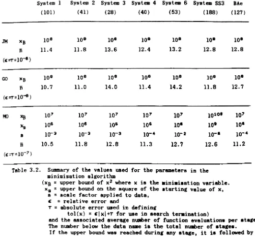
programs used one or the other subroutine for the optimisation. 7 Bet.s of data have been used to test the performance of t.heBe al,orit.h.B. The 7

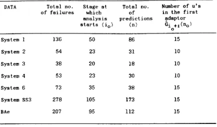
8ets of data are System 1, Syst.em 2, System 3, System 4, SYBtem 6 and

System SS3 from Musa (1979) and BAe data from British Aerospace. These

with considerable insight into the behaviour of the MLE of the paramet.ers in each model. Furthermore, it is on the basis of the difficulties we have encountered during these test.s t.hat we incorporate certain chan.res to our original minimisation algorithms to make them more efficient for the more

difficult problems. We begin by lookin.r at the univariate problems first.

JM and GO model programs performed very well across all 7 data 8ets. However a potential difficulty exists in GO which is partly ori.rinated from t.he data it.self.

There are often no dimensions ,iven for aoftware reliability data. They usually come as a sequence of numbera which mi,ht have already been scaled in some way which is convenient for recordin, and aecurity.

Therefore, the magnitudes of two sets of data can be very different, even

if the programs are equally reliable, just because the data have been aealed differently. For example, it is fairly obvioua that the ma,nitude of the failure times in System SS3 is bi,ger than that of Sy.tem 1, but if one multiplies the inter-failure times in Syatem SS3 by a factor of 10-' t they

would not look so dissimilar in magnitude anymore. Some but not all of the parameter8 in a software reliability model are aeale invariant, i.e. the magnitude of the parameter does not chan.re when a po.Uive aeale ia applied to the data. Therefore the ma,nitude of t.hoae which are variant to aeale will depend on the acale of the data.

Reeall t.hat in the caae

ot

GO model t.he minimiaation variable ia x

=

*,.,..:

which is usually very amall. Alao recall that the aearch will terminate if max[ b-x,x-a) ( 2tol(x) wit.h tol(x)

=

c

I

x

I

+T

a.

defined in