Preliminary Interdependency Analysis (PIA): Method and tool support

(1)

City, University of London Institutional Repository

Citation

:

Bloomfield, R. E., Chozos, N., Popov, P. T., Stankovic, V., Wright, D. and Howell-Morris, R. (2010). Preliminary Interdependency Analysis (PIA): Method and tool support (D/501/12102/2 v2.0). London: Adelard LLP and City University London.

This is the unspecified version of the paper.

This version of the publication may differ from the final published

version.

Permanent repository link:

http://openaccess.city.ac.uk/3091/

Link to published version

:

D/501/12102/2 v2.0

Copyright and reuse:

City Research Online aims to make research

outputs of City, University of London available to a wider audience.

Copyright and Moral Rights remain with the author(s) and/or copyright

holders. URLs from City Research Online may be freely distributed and

linked to.

(2)

Preliminary Interdependency

Analysis (PIA): Method and tool

support

© Adelard LLP and City University London, 2010

(3)

(4)

Summary

This report is the second deliverable of the TSB-funded PIA:FARA project. The report presents a method called Preliminary Interdependency Analysis (PIA) which can be used to conduct interdependency analyses in complex systems such as Critical Infrastructures. The method is supported by a toolkit which can be used to conduct qualitative and quantitative analyses of interdependencies between complex systems.

Authors

R Bloomfield N Chozos P Popov V Stankovic D Wright

(5)

Document control

Reference: D/501/12102/2 Status: FINAL

VERSION REVIEW NO./ISSUED DATE

v0.1D issued in draft 19 May, 2010 v0.1J R/1890/12102/4 21 June, 2010 v1.0 issued 23 June, 2010 v1.1A R/1969/12102/5 11 November, 2010 v2.0 issued 15 November, 2010 Approved: Robin Bloomfield

Verified: Fan Ye

Distribution

Alan Bennett, Technology Strategy Board Monitoring Officer Paul Lewis, Technology Strategy Board

(6)

Figures

Figure 1: Overview of PIA method and toolkit... 9

Figure 2: PIA method stages ... 12

Figure 3: Example views used in PIA... 14

Figure 4: A Coupling point as a link between services in PIA ... 16

Figure 5: UML component diagram of the PIA toolkit... 28

Figure 6: Interconnectivity matrix plug-in ... 29

Figure 7: Google Earth plugin... 30

Figure 8: A state machine diagram for a local telephone exchange and the links status-fields editor plug-in ... 37

Figure 9: Part of the intra-service PN view of the Power Transmission service... 37

Figure 10: A part of the SAN of the Telco SDH service... 38

Figure 11: The “Node search” plug-in ... 38

Figure 12: The Network status-field editor plug-in... 42

Figure 13: The HTML form used for the validation when creating a new PIA project... 42

Figure 14: The Link status-field editor plug-in ... 45

Figure 15: The Generate State Space values plug-in... 46

Figure 16: The status-fields for the node MVC1 of an Intra_PN ASCE network... 47

Figure 17: The Inter-service links (coupling points) plug-in ... 49

Figure 18: The Physical Network views import plug-in ... 51

Figure 19: The plug-in used for configuration of the Möbius-based simulation study... 53

Figure 20: The plug-in used for specifying the particular execution order of Deterministic plug-ins in a PIA project... 53

Figure 21: The plug-in for mapping entities defined in a Deterministic plug-in to entities from the PIA project... 54

Figure 22: The plug-in for generation of the Möbius-based simulation project ... 56

Tables

Table 1: CI/service definitions for an information infrastructure ... 14

(8)

1 Introduction

One of the greatest challenges in enhancing the protection of Critical Infrastructures (CIs) against accidents, natural disasters, and acts of terrorism is establishing and maintaining an understanding of the interdependencies between infrastructures and the dynamic nature of these interdependencies. Interdependency can be a source of “unforeseen” threat when failure in one infrastructure may cascade to other infrastructures, or it may be a source of resilience in times of crisis, e.g., by re-allocating resources from one infrastructure to another [1].

Understanding interdependencies is a challenge both for governments and for infrastructure owners/operators. Both, to a different extent, have an interest in services and tools that can enhance their risk assessment and management to mitigate large failures that may propagate across infrastructures. However, cost of investment in infrastructure modelling and

interdependency analysis tools and methods, including the supporting technology, may reach millions of pounds, depending on the size of the system to be modelled, on the level of detail and on the mode of modelling (real-time or off-line). These factors will determine the software, hardware, data and personnel requirements.

It is therefore very important to understand what the scope and the overall requirements of an interdependency analysis service are going to be, before proceeding with such an investment. However, the decision on what modelling and visualisation capabilities are needed is far from simple. Detailed requirements may not be understood until some modelling and simulation has been conducted already, in order to identify critical dependencies and decide what level of fidelity is required to investigate them further.

This report presents an approach to interdependency analysis that attempts to address these challenges. The approach—Preliminary Interdependency Analysis (PIA)—starts off at a

high-level of abstraction, supporting a cyclic, systematic thought process that can direct the analysis towards identifying lower-level dependencies between components of CIs. Dependencies can then be analysed with probabilistic models, which would allow one to conduct studies focussed on identifying different measures of interests, e.g. to establish the likelihood of cascade failure for a given set of assumptions, the weakest link in the modelled system, etc. If a high-fidelity analysis is required, PIA can assist in making an informed decision of what to model in more detail. The method is applicable as both i) a lightweight method and accessible to Small-to-Medium Enterprises (SMEs) in support of their business continuity planning (e.g., to model information infrastructure dependencies, or dependencies on external services such as postal services, couriers, and subcontractors); and ii) a heavyweight method of studying with an increasing level of detail the complex regional and nationwide CIs combining probabilistic and deterministic models of CIs.

This deliverable illustrates the use of PIA on a case study (Appendix B): a regional system of two CIs namely the power grid and telecommunication network around Rome, Italy (i.e. Rome case-study).

PIA is supported by a toolkit. The PIA Toolkit consists of two software applications:

(9)

● The Execution engine, which allows for executing a model developed with the PIA

Designer, i.e. a simulation study based on the model to be conducted and the measures of interest to be collected. The Execution engine uses Möbius [12], customised extensively

with a bespoke proprietary development.

The current version of the toolkit allows for two main categories of models:

● Model of interdependent CIs at a fairly high level of abstraction (i.e. without detailed modelling of the networks used by the respective services). The model can be parameterised and then the simulation executable can be deployed on the Execution Engine.

● As above but adding any degree of detail that the modeller may consider necessary including high fidelity deterministic models available as 3rd_{party software modules.} This report presents the PIA method and offers a detailed description of how the PIA Toolkit can be used.

2 Method: Preliminary Interdependency Analysis (PIA)

Preliminary Interdependency Analysis (PIA) is an analysis activity that seeks to understand the range of possible interdependencies and provide a justified basis for further modelling and analysis. Given a collection of CIs, the objectives of PIA are to develop, through a continuous, cyclical process of refinement, an appropriate service model for the infrastructures, and to

document assumptions about resources, environmental impact, threats and other factors. PIA has several benefits. In particular, PIA can

● help one to discover and better understand dependencies which may be considered as “obvious” and as such are often overlooked (e.g. telecommunications need power)

● support the need for agile and time-efficient analyses (cannot always wait for the high fidelity simulation)

● be also used by Small-to-Medium Enterprises (SMEs) and not just infrastructure owners and government

PIA allows for the creation and refinement of interdependency models, in a focused manner, by revisiting earlier stages in the PIA process in the light of the outcomes of latter stages. For example, an initial application of PIA should result in a sufficiently concrete and clearly defined model of CIs (and their dependencies). However, following the first design iteration, an analysis of the model could cause us to question the assumptions made earlier on in the design process. As a consequence, the model may be revised and refined; as we shall see later on, revisiting previous phases of the development process is a key aspect of the PIA method and philosophy overall.

PIA consists of two parts:

● Qualitative analysis. The modelling exercise begins with a definition of the boundaries of

the system to be studied and its components. Starting off at a high level, the analyst may go through a cyclical process of definitions, but may also be focused on a particular service, so the level of detail may vary between the different parts of the overall model. The

identification of dependencies (service-based or geographical) will start at this point.

● Quantitative analysis. The models created during the qualitative PIA are now used to

(10)

of the modelled entities for the chosen model parameterisation. The model parameterisation may be based either on expert judgement or on analysis of incident data. Examples of such data analyses and fitting the available data to plausible probabilistic data models was presented in the recent WP1 deliverable [2].

The PIA Toolkit provides support for both the qualitative and quantitative analyses. Figure 1 illustrates an overview of the method and the toolkit.

Quantitative PIA

- Setting system boundaries - Service definition (inputs, output external resources)

- Identification of service parts (components, assets, internal resources)

- Identification of dependencies between services and their parts

- Definition of state-machines (states and transitions) - Parameterisation of stochastic associations

- (optional) Adding and configuring plug-ins - Deploying model on the execution engine

- interdependency study via simulation

Scope and boundaries Threat models Incident data

Run-time Model Description

- A complete Möbius project - A set of text files - Utilities, plug-ins

Execution Engine

A Möbius compatible simulation environment

Qualitative PIA

PIA Designer

Graphical model development with the

[image:10.595.124.481.206.537.2]

ASCE tool

PIA

Method

PIA

Toolkit

Deployment

Figure 1: Overview of PIA method and toolkit

The interdependency models, of course, have to be related to a purpose and this should be captured in terms of a scenario and related requirements. The narrative aspect of the scenario is enormously important as it provides the basis for asking questions and discovering

interdependencies as the starting point for more formal models.

Typically the systems of interdependent CIs of interest are complex: include many services which in turn consist of many parts. Given the complexity and size of the analysed systems tool support is essential. The aim of WP2 is therefore to produce a toolkit that supports PIA

(including both qualitative and quantitative stages).

2.1 PIA model architecture: two levels of abstraction

(11)

● Model of interacting services (service-level model). The modelled CIs are represented by a

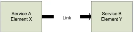
set of interdependent services. Here, the view is purposefully abstract, so that we can reason about dependencies among the services (i.e. data centre X depends on power plant Y). Service-level dependencies are elicited by the defined lower-level dependencies among each service’s constituent entities (physical components, resources etc.). These associations among components are referred to within PIA as coupling points. The coupling points incoming to a service can be associated with the resources that the service requires (e.g., a

telecommunication service consumes “commodities” supplied by a power service). The resources consumed by a service can be obtained from the organisation’s reserves (internal resources) or provided by another organisation (external resources). The outgoing coupling

points instead define how the outputs from a service get consumed by other services (as either inputs or resources).

● Detailed service behaviour model (DSBM). Implementation details are provided for an individual service, e.g. the networks upon which a particular service relies. For instance a

Global System for Mobile (GSM) telecommunication operator typically relies on a network of devices deployed to cover a particular area (e.g. masts, etc.). Via DSBM we can choose the level of detail used to model these networks. In the example above DSBM may range from a connectivity graph – which cells of the network are connected with each other to a high fidelity model of the protocols used in the GSM network. We tend to think of DSBM as the networks owned (at least partially and/or maintained) by the respective service operator, i.e. an organisation. Although such a view is not necessary, it allows one to model several important aspects via DSBM. For instance the level of investment and the culture (strong emphasis on engineering vs. outsourcing the maintenance) within the organisation will affect how well the network is maintained (i.e. frequency of outages and speed of recovery). Thus, the process of recovery (a parameter used in DSBM) can be a useful proxy of the level of investment. Thus, through DSBM one can study scenarios which at first may seem outside the scope of PIA. An example of such a scenario would be comparing the deregulation with tight regulation in critical CIs.

2.2 PIA stages

PIA is carried out in seven stages (Figure 2):

Stage 1. CI description and scenario context (Section 2.2.1). A CI description provides a

concrete context and concept of operation. This is the first level of scoping for the analysis task; the CI description gives the first indications of analysis boundaries. DSBM entities are identified and recorded.

Stage 2. Model development (Section 2.2.2). A model of the services (resources, inputs,

outputs, system states) and the operational environment and system boundaries are developed, based on the CI description. Model boundary definitions are used at this stage to further restrict the scope of the analysis. Dependencies between the services are identified and the coupling points are defined: these refer on the one hand to the

inputs and resources required by each of the services and on the other hand to the outputs that each of the services produces.

Stage 3. DSBM model development (Section 2.2.3). DSBMs are defined by selecting the

right level of abstraction for the services: some of the services may be treated as black-boxes; in this case their representation in the DSBM will require no

(12)

by the services or use other formalisms, e.g. such as PVS [9]. A level of consistency is achieved between the service model and DSBM: the coupling points appear in both Views.

Stage 4. Initial dependency and interdependency identification (Section 2.2.4). While some

of the service dependencies have already been identified and recorded in Stage 2 (via input/output/resource identification), at this stage the modeller looks for additional sources of dependence (e.g. common components/assets), which may make several services vulnerable to common faults or threats. These can be derived by examining the service-level model, taking into account other contextual

information (e.g. scenarios, threat models, attacker profile). The captured dependencies are modelled as stochastic association between the services or

components thereof. Each stochastic association is seen as a relationship between a parent and a child: the state of the parent affects the modelled behaviour of the child.

Stage 5. Probabilistic model development (Section 2.2.5). Since we are dealing with risk, we

take the view that, given the state space formed by the modelled entities (MEs), a stochastic process must be constructed upon it that captures the unpredictable nature of the states of the MEs, their changes and the interactions between CIs over time. In this stage probabilistic models of the MEs are defined. These are state-machines,

a well known formalism in software engineering, modelled after the formalism used in the Stochastic Activity Networks (SANs).

Stage 6. (optional) Adding deterministic models of behaviour (Section 2.2.6). At this stage

the modeller may decide to extend the behaviour of the probabilistic model adding deterministic models of behaviour. Such a step may be useful when the modeller is seeking to extend the fidelity of the simulation beyond the standard mechanisms possible with a pure probabilistic model.

Stage 7. Exploratory interdependency analysis (Section 2.2.7). A Monte Carlo simulation

[10] is used to quantify the impact of interdependencies on the behaviour of the system under study and draw more conclusions about the probability of

(13)

Stage 1

CI description / Scenario context Scenarios

Stage 7

Exploratory Interdependency

Analysis

Stage 6

Deterministic Models Configuration

Stage 4

Identification of dependencies

between services

Stage 2

Service level model development

PIA stages

Incident description

Threat or attack model

Model of threat agent

Stage 5

Probabilistic parameterisation

Stage 3

DSBM level model development

Deterministic Models

No

[image:13.595.155.441.95.676.2]

Yes

Figure 2: PIA method stages

(14)

● Scenarios: PIA is a scenario-driven approach. Once the system has been modelled,

“what-if” questions will be used to explore vulnerabilities and failure cascade possibilities. Scenarios can be developed from a variety of assumptions or experiences. For instance, one can begin by asking a question as abstract as “what happens if there is a flood”, or “if power plant X fails”. Such questions form the basis for scenarios, which focus the analysis on particular conditions, exploring potential vulnerabilities.

● Incident description: PIA can be used to model an incident that has already occurred. This

can be used as a baseline for generating and exploring variations of the same scenario or simply further exploring a system that has been compromised, or has failed, as the incident revealed unpredicted vulnerabilities and failures.

● Threat or attack model: Here, we are considering modelling assumptions based on

malicious attacks.

● Model of threat agent: The above (scenarios, incident description, threat or attack model)

are elements that will shape the profile of a threat that is modelled in our system. This can be a malicious agent (e.g. a terrorist) or a source of natural disaster (e.g. flood).

The seven stages are described in more detail in the following sections.

2.2.1 Stage 1: Critical infrastructure / Service description

2.2.1.1 Definitions

A service provider (typically an organisation or a company) provides a service. Typically the

service provider utilises a network, which in turn consists of components that use resources to

provide an output. The relationship ‘whole-parts’ between a service and its parts (components,

internal resources and assets) is explicitly modelled at this stage.

Loss events occur when the service is interrupted, either by a component failure or by

exhaustion of resources. Measures of interest which will be studied are also identified and recorded at this stage.

The definition of the service and of its parts alone will be a useful process as it will help identify the boundaries of the system to be modelled, and the usually abstract initial understanding of some obvious dependencies will begin to become clearer. However, these definitions need to be coherent, as the subsequent modelling and analyses will be based on them. We would expect that the definitions would be developed by a team of experts, possibly from various levels within the service organisation; this is because during the development of definitions we consider both high-level views (e.g., production of energy) and low-level views (e.g., identification of specific physical components), and most importantly, how they are related. Similarly to other modelling approaches (most notably UML1_{) PIA uses}

different views which

allow the modeller to deal with complexity (i.e. separate concerns) and switch easily the focus of analysis from dealing with the whole to dealing with its parts and from modelling the entities of concrete critical infrastructures (with their concrete engineering meaning) or to the

description of the probabilistic behaviour. The figure below gives an example of views which we found to be useful in practice (Figure 3).

1 _{Unified Modelling Language (UML) is a standardised general-purpose language for modelling}

(15)

Service-level view

(the service that the infrastructure is providing)

Implementation-level view

(the sum of components that make up the infrastructure)

Application-level view

[image:15.595.175.421.103.273.2]

(the utilisation of the infrastructure in order to provide the service)

Figure 3: Example views used in PIA

Below we elaborate further on the use of the views listed in Figure 3, based on the work on an ongoing case study which considers the information infrastructure of an SME.

View Description

Services ● Production and delivery of reports ● Help-desk

● Licensing

● Invoicing

Application ● Access to data and information (read-only)

● Modification of data and information (create, modify, delete, save)

● Communication (face-to-face, telephone, email etc)

Implementation ● Hardware ● Software

● Data

● People

Table 1: CI/service definitions for an information infrastructure

What is presented in this table is the first layer of definitions for the three views. Following several iterations this leads to a rather detailed list of individual components, such as servers, hubs, databases and people. As mentioned previously, this process will require the involvement of people from various levels of the service organisation, so that the link between the service-level view and the implementation-service-level view can be achieved.

[image:15.595.106.491.346.557.2]

(16)

2.2.1.2 PIA elements

Component Definition

Service organisation

A service with certain characteristics is provided by a service organisation. The service is essentially a label for the process of transforming the resources into a saleable commodity.

This is the highest level of abstraction for defining physical components. Service organisations may be power plants, data centres, airports, etc.

Component A component is a commodity, part of the service, which is used in the

transformation of resources into a product. Components may fail in operation, either as a result of wear and tear (physical hardware elements) or design faults (software, hardware, procedures), in which case the service output may be affected. Whether the component failure will affect the service output depends on the service’s internal resilience (its ability to withstand component failures, e.g. as a result of fault-tolerant design).

An important aspect to consider when dealing with components is that they may be geographically dispersed, forming a distributed network of

components. In addition, in many cases, considering people as components in the model is a sensible strategy.

Asset An information asset (e.g. technical know-how, data, procedures, algorithms) is

used either directly or indirectly to produce a product. The information assets may be stolen, misused or corrupted as a result of accidental failure or malicious behaviour, in which case the supplying organisation may be

adversely affected. Assets can be electronic or paper-based records and files, or softer aspects such as trust and reputation.

Resource Resources are being consumed. They are supplied by internal reserves or

external services. External resources are commodities which are normally consumed in the process which leads to the supply of a product at the service output. This consumption is important as it can be a source of hidden

dependencies. Electrical power, air conditioning as well as consumables would fall under this category.

Input The input to a service is the demand for a given product. Demands can come

from other services, the public, legislation, governmental directives, etc. The demand is seen here as a request for a service based on an agreement of some sort (such as a contract between the supplying organisation and the consumer).

Output An output is a product of a modelled component.

Environment In most cases, under “environment” we would expect to see aspects of weather

[image:16.595.78.516.116.648.2]

and other natural phenomena (e.g., earthquakes).

Table 2: PIA elements

Producing a set of coherent definitions may require several iterations. We recommend that these are recorded in a systematic, clear manner, as these definitions will determine the outcome of the rest of the modelling and analysis.

2.2.1.3 Service state

The state space of a modelled service is defined either explicitly or implicitly. The explicit

(17)

further refinements detailing its parts are used. In this case the modeller would associate the service with a state machine in which the possible service states are spelled out.

We found that in the case of explicit definition of a service it might be useful to consider a minimalistic state space {OK, impaired, failed} so that the modeller can distinguish between the possible degrees of operability (from fully operational (OK), to totally non-operational {failed}, impaired denoting partial operability).

In the case a DSBM is associated with a service, the service state is implicitly defined by the state spaces of its parts: components, internal resources and assets. In this case the modeller is expected to define the state of the parts, but no explicit definition of state machine associated with the entire service is required; the service state space is the Cartesian product of the state spaces of its parts.

2.2.1.4 Scope and boundaries

Building a model of interdependent CIs typically requires multiple iterations of refinement: starting with the definition of the services and how they are interdependent (input, output, resources) at a higher level of abstraction and then gradually progressing by adding details, e.g. DSBMs for the services judged to require a more detailed description. DSBMs themselves can be refined multiple times – possibly driven by the results obtained from the previous iterations of refinement.

Our practical experience with PIA has been with geographically compact studies – a critical information infrastructure of an SME and a regional study of two interdependent CIs. The particular types of modelled entities are dictated by the context of the study. These may include a set of hardware components, e.g. the ones used in the telecommunication and in the power grid CIs in the case of the regional system case that we started studying in IRRIIS [6] and the entities of the information infrastructure of an SME in an ongoing case study.

2.2.2 Stage 2: Service-model development

In this phase, the dependence between the services modelled are identified: input/external

resource – output relationships, the components (e.g. of the same type such as a PC running the same OS and application software) which may be subject to common mode/cause failure, or stochastic associations are identified and marked as coupling points(see Figure 4) between the

[image:17.595.183.414.577.634.2]

services.

Figure 4: A Coupling point as a link between services in PIA

(18)

2.2.3 Stage 3: DBMS model development

This stage is focussed on developing the DSBM models (i.e. detailed inter-service models) for those services chosen to be modelled in detail. The parts that make up the service (components, assets, internal resources) defined in Stage 2 are now scrutinised and their associations

(deterministic and stochastic) are identified and represented in the DSBM.

At this stage we define the state-machines used to model the behaviour of the modelled entities. The services for which no DSBM is defined will be associated with a state-machine which will define the states and the state changes of the entire service.

In case a DSBM is associated with a service, the modeller is expected to define a separate state-machine for each of the service’s parts. The state of a service in this case is represented by the Cartesian product of the states of its parts.

2.2.4 Stage 4: Identification of dependencies between the services

At this stage the analysts proceeds by asking ‘what-if’ questions and exploring particular threat models and scenarios which may cross the service boundaries.

Apart from the obvious dependencies (e.g., telecoms need power), which may be observed by considering the functional association between entities, there are some other aspects of CIs that need to be taken into account. The following are some key concepts that should be considered in threat models and scenarios:

● Geographical dependencies. Vulnerabilities may lie not only in functional dependencies

between components, but also in the risk of, for example, an explosion occurring in a nearby site. Recording the geographical information for each element is done in the stage of Service Description (Section 2.2.1.3). At design time we can identify and record, e.g. using a special link type “near to”. However, such an approach will be of limited value. It will identify some and will miss many interdependencies due to geographical proximity. Our experience indicates that a systematic study of the impact that geographical proximity will have on interdependencies between the services will require a combination of static analysis and (simulated) stochastic modelling whereby the anticipated disruptions (earthquakes, flooding, sabotage, etc.) are instantiated at randomly chosen location and with a random severity (e.g. magnitude of the earthquake). Implementing such an approach via static analysis may be less effective than using a simulation with a randomly generated location of the disruption and a randomly generated area affected by the disruption.

● Competition for resources. During a crisis, dependencies may become apparent between

entities that share the same resource(s). When more than one element reallocate their resources (e.g. maintenance personnel), there may be competition between them. This may lead to starvation of the particular resource, or the accumulation of dependencies to one element, which will then be bearing the risk of causing multiple disruptions, should that fail too.

● Resilience perspective. The failure of one element may have an indirect effect on another

during a crisis if it compromises a resource, a component or an asset that are critical to its recovery. This is the kind of dependency that may not be visible during normal operation.

● Common mode/cause models. The modeller should also look for additional sources of

(19)

example of common vulnerability is the use of several PCs of exactly the same type (the same hardware specs, OS and set of applications). In this case one is justified in making a modelling assumption that an actual failure or compromise of a component of the particular

type in one of the services implies that the other components of the same type in either the same service or in other services become more likely to fail or be compromised than before

the failure of the first component occurred2_.

The captured dependencies get modelled probabilistically in the form of stochastic associations,

which can occur between the services or components thereof depending on the level of abstraction used. Each stochastic association is seen as a relationship between a parent and a child: the state of the parent via the stochastic association affects the modelled stochastic

behaviour of the child. The stochastic association is characterised by its strength. For example,

using a stochastic association between parent A and child B, the modeller can define that the rate of failure of B will increase 10-fold (in this case we say that the strength of the association is set equal to 10) when A is in a failed state in comparison with the rate of failure B when A is working correctly.

When considering modes of behaviour (i.e., how a failed or impaired element impacts the rest of the model), the temporal aspect needs to be taken into account. Dependencies, especially when considering competition for resources or recovery, may arise over time. Vulnerabilities may start becoming obvious as resources or the capacity of a system reach their limits. Modelling these temporal aspects is important.

Incident history should be taken into account when asking what-if questions, as previous incidents can help unveil similar and/or related scenarios.

2.2.5 Stage 5: Probabilistic parameterisation

Our method of quantifying interdependencies is based on a combination of techniques outlined in greater detail in [6]. A key problem is to define mechanisms of association between distinct MEs, whereby the model is given a structure that is realistically different from the rather limited concept of a number of state-holding MEs, embedded in a common simulated time line,

behaving independently, as parallel stochastic functions of simulated time. Rather, we require a definition of a multivariate stochastic process of states of the MEs, representing the MEs’ interactions with one another: interaction which may be deterministic (discussed in stage 7), or which may be probabilistic in the sense that the states of MEs, and perhaps also transient

environmental stresses and perturbations, will influence the risks to which other MEs are subject in precisely defined ways. Every event that an ME may manifest, will take the form of a

transition between two states of its assigned state space. As a result, the stochastic process to be modelled is of significant complexity, which makes Monte Carlo simulation [10] the preferred

model analysis technique. We have built a generic tool, based around the simulation solver of the Möbius SAN tool [3][12] (see Appendix A for an overview of the tool), augmented by additional code of our own design, to conduct such simulations. These take the form of

continuous time, discrete event driven simulations of CI behaviour and interaction, represented as sequences of changing states of MEs.

We use the notion of a type of modelling entity (TME). A separate state-machine is defined for

every TME. The modelled system, however, may include multiple instances of the same TME,

2_{We note in passing that elsewhere we provided an extensive justification of the plausibility of this}

(20)

which will share the same state-machine (number of states and transitions between the states). The probabilistic description of the instances, however, may be unique – the SAN model associated with the instances of TME may be different (i.e. the probability distributions associated with the transitions of the state-machines) for the different instances.

At this stage the modeller provides probabilistic parameters related to the transition parameters of the state-machines which model the behaviour of the modelled entities. The modeller can specify a unique set of parameters even if two modelling entities are of the same type (i.e. share the same TME). The following set of parameters must be provided:

● the model of transitions (competing risks is the default for SAN) and unless there are good

reasons to use a different model we would use the default

● the type of distributions which characterise the transitions from the current state to any possible next state (exponential, Weibull, or other probability distributions)

● the parameters of the specified distribution (e.g. the rate parameter of an exponential distribution).

Also parameterised at this stage are the stochastic associations between the MEs, i.e. the associations’ strengths. In the current implementation of the toolkit we assume that the effects of multiple parents of the same child are independent of each other. The design of the toolkit,

however, allows for implementing non-independent stochastic associations.

Once the parameterisation is completed, the modeller can study the effect of systematic

parameter variation on the behaviour of the model as a whole. For each assignment of parameter values, an experiment is undertaken. This allows the effect of the parameter on the variability of defined CIs properties, e.g. such as the frequency of large incident cascades or outages of service, to be obtained.

2.2.6 Stage 6: (optional) Adding deterministic models of behaviour

At this stage the modeller may decide to extend the model description by adding deterministic models which increase the fidelity of simulation and will be difficult to represent using the stochastic model only. For instance, the use of such models will allow for propagating in detail the consequences of failures or repairs of the modelled entities. Good examples of deterministic models are the flow models (e.g. DC/AC power flow models, various telecommunication traffic models, etc.).

(21)

A point worth mentioning here is that although the pluggable architecture was designed with deterministic plug-ins in mind, it can be used to implement any functionality, including probabilistic extensions, which are difficult to define statically. For instance, the model of environmental disturbances (earthquakes, flooding, etc.) discussed in Section 2.2.4 may be modelled using plug-ins which would determine at random the location and the magnitude of the event, thus making it possible to model the disturbance with a simple state-machine with states (active, inactive).

2.2.7 Stage 7: Exploratory interdependency analysis

In order to carry out the exploratory interdependency analysis, Monte Carlo simulations [10] are used. For each experiment, a number of replications of the evolution of the model, using

identical parameters, over a defined interval of simulated time, may be conducted. One

replication of an experiment differs from another solely in that the random number generator is seeded at a different starting point. Then statistical sampling theory may be used to study the distribution properties of system measures of particular interest for each set of assigned parameter values.

The focus of the studies is defined in the so called reward variables, the values of which are

computed at simulation time over the states of the SAN model implemented by a Monte Carlo simulator. The same model can be executed with a number of rewards. There are two groups of simulation activities:

● Calculating statistics on the defined rewards based on multiple repetitions of a simulation, e.g. comparison of distributions of important CI dependability summary statistics between experiments with different parameterisations and/or level of abstraction. Typical examples here are:

● Sensitivity analysis with respect to a particular model parameter (e.g. how the variation of the strength of stochastic association affects the results)

● Distribution of cascades (i.e. outages that include more than one modelling entity) ● Using the simulation traces obtained from the history of a single experiment over a long

interval of simulated time may be searched for interesting features. Examples of analyses of this kind include:

● Searching for cascade failures and scrutinise these to understand better the “mechanisms” of cascades or use these in training.

(22)

3 Tool support: PIA Toolkit

The qualitative part of the method described in this document could be applied without the use of tools. However, such an activity would be both more resource intensive and failure prone, since e.g., the application of the method will need to be performed specifically for each new PIA study without a possibility of reuse. In any case, the quantitative part does require the use of tools.

In the past we relied on two separate tools: ASCE for the qualitative part of the analysis and Möbius SAN for the quantitative part (a short description of each tool is given in Appendix A). The main objective for WP2 in the PIA:FARA project was to develop a toolkit which would allow a modeller to progress seamlessly from qualitative to quantitative interdependency analysis. More specifically, in WP2 we set out to achieve the following:

● Development of models of interdependency between CIs in a graphical environment. This is achieved with the PIA Designer toolwhich:

1. allows the modeller to switch between different views dealing with the different stages

of modelling as described in Section 2. This includes being able to easily change the modelling assumptions and the model parameters used for the quantitative analysis. 2. offers support of the pluggable architecture of the run-time engine (i.e., execution

engine, see the following paragraph) whereby an executable (to conduct quantitative interdependency analysis by simulation) would be configured to use the simulation plug-ins needed in a study before deployment of the simulation executable on the run-time engine.

● Performance of probabilistic analyses based on the graphical models developed with the PIA Designer. This is achieved with the software tool referred to as Execution Engine, which has an architecture that separates the quantitative analysis tasks common to all PIA studies (such as SAN models of the modelled entities and their stochastic associations) from the specifics of the particular study (e.g., optional add-ons needed only in some PIA studies, specific parameterisations of the stochastic associations, etc.). This objective was achieved by adopting a pluggable architecture in which software modules compliant with the architecture can be easily added to a study by configuring the simulation study.

Below are some of the ways in which the PIA Toolkit can enhance the application of the PIA approach:

● Visualisation. PIA models are enhanced with graphical representation. Visualisation can

assist in the visual exploration of system dependencies and, when combined with geographical information, support the thought process for considering disaster scenarios such as flood or earthquake. ASCE has a powerful and flexible graphical modelling environment; in addition, PIA Designer has the capability to export the modelled system to

Google Earth [9] application if geographical coordinates have been entered as attributes

(status fields in ASCE terminology) of the constituent model entities. Visualisation can also

be used to facilitate communication among different analysts and other stakeholders as they are looking at the graphical models. Model views created in PIA Designer are hereafter also referred to as ASCE networks (adopting the jargon used by the ASCE tool developers and

(23)

● Analysis automation. Mathematical modelling is aided, and parts of it are automated

through the integration of the tools for qualitative and quantitative analysis in the PIA Toolkit.

A significant part of the PIA Toolkit development has involved the work on integration of the PIA Designer and the Execution Engine. This work aims to deliver a seamless integration between the two parts of the toolkit—the user interacts with PIA Designer as the front-end of the toolkit, with only the minimal need for interaction with the Möbius-based execution engine. After the user finishes with the PIA model development in PIA Designer, the necessary

information is communicated to the Execution Engine, so that probabilistic model is initialised and the simulation is executed.

In this section we give a description of how the PIA Toolkit is used to support the PIA method with the benefits of visualisation and enhanced analysis features, as well as present the

architecture of the toolkit.

3.1 PIA Toolkit Usage Patterns

In general, we envisage two approaches to development of PIA models:

● Interactive analysis performed “from scratch”, whereby the analyst is building the PIA model afresh by going through the PIA stages as described in Section 2.2. In this way, the PIA Toolkit user would generate the model views manually, in a step-by-step manner: creating the necessary physical entities belonging to the CI services under scrutiny, assigning the required parameter values to these entities, creating and parameterising stochastic associations etc.

● Automated analysis, whereby the analyst is using pre-existing data sets about the modelled system to programmatically produce initial graphical representations of it. This approach is suitable when, for example, a description of a real incident is available. In such cases, some software utilities that are part of the PIA Toolkit can help generate ASCE networks

belonging to a particular PIA study.

In both cases, the PIA stages as defined in Section 2.2 are followed. However, depending on the amount and the format of the data sets available, the analyst will have to go through a series of steps where interaction with the tools will be required. It should be noted that these two PIA development approaches are not necessarily mutually exclusive, i.e. the Interactive and Automated analysis might be combined inside a single PIA study.

3.2 Overview of PIA workflow

This sub-section provides a software-centred description of the steps taken when using the PIA Designer to accomplish a series of tasks necessary for the development of a PIA model. It explains typical usage of the PIA Designer software.

The user of PIA Designer, PIA Analyst, can generate two broad categories of the PIA model representations, i.e. model views: Intra- and Inter-CI service views. The former depicts the

associations between the entities of the same CI service, while the latter depicts the associations across CI service boundaries. An orthogonal categorisation of the model views is as follows:

● Physical Network (PN) view, which depicts the physical entities (physical nodes or physical

(24)

transmission service, we would for example include voltage cabins as nodes and high-voltage trunks as links among the other kinds of entities the service might consist of).

● Stochastic Associations (SA) view, which is a representation of the stochastic associations

(see Section 2.2 for anexplanation of the term)between the model entities.

The interaction between the PIA Designer software and its user consists of the following sequence of steps:

Step 1. Create Notational Schemas. By executing this step the PIA Analyst creates the

necessary ASCE schemas that are used as the basis for developing ASCE networks

(see Appendix A) used in the PIA model. For example, a notation for describing the Intra-PN view of each service modelled in the PIA study will need to be developed.

Step 2. Create PIA Project network. PIA Analyst then creates PIA Project network which is

used to maintain the references to all ASCE networks belonging to a particular PIA model. Every PIA Project has a default set of ASCE networks. The set of default

networks includes: Inter-PN, Inter-SA, StateTransitions and SimulationPlugins

networks. For more information see sub-section C.1 in Appendix C.

Step 3. Populate State Transitions network. The user creates the state machines for all the

entity kinds, i.e., all TMEs (see Stage 5 in Section 2.2) used in the particular PIA model. For example, if the PIA was applied to a Public Switched Telephone Network (PSTN) CI, then the set of TMEs could include the following: Backbone Exchange, Transit Exchange, Local Exchange etc.

A state machine for each TME consists of the set of states and the associated state transitions. Each state transition needs to be parameterised. The state transition parameters include the i) Function_type – the family of functions this state transition

belongs to, ii) Function_name – the particular function used for the state transition and

iii) Function_parameters – the parameters that the state transition function accepts.

Initially, every entity instance of a particular TME takes on the default state transitions values. The PIA Analyst can, however, specify a set of parameters for a particular entity instance which is different than the default one. For more information see sub-section C.2 in Appendix C.

Step 4. Populate Physical Network (PN) networks. This step consists of the following two

activities:

Populate Intra PN networks. This is the central point of the development, or

refinement, of the PIA model of any of the services: it processes the topology information of physical networks of each modelled CI service to create respective graphical representations (i.e., ASCE networks). Each such network is based on the notation, i.e., ASCE schema, created in Step 1. These networks consist of a possibly large number of entities and thus the visual representation aids in comprehending their complexity.

Populate Inter PN networks. This activity is based on the definition of the coupling

(25)

precisely causally affects, at least one entity from another service, while in an SA ASCE network the attribute defines if an entity is stochastically associated with at least one entity from another service (see Section 2.1 for further explanation of the coupling points term).

For more information about this step see sub-section C.3 in Appendix C.

Step 5. Populate Stochastic Associations (SA) networks. This step includes the following: Populate Intra SA networks. During the execution of this step the stochastic

associations between the entities of the particular, i.e., “native”, CI service are identified and the values of the parameters of each association are specified. In

addition, in the Intra-SA view the stochastic associations affecting entities belonging to other, i.e. “foreign” CI services are identified if an entity, say EN, from the native CI stochastically affects an entity, say EF, from a foreign service, i.e., EN is stochastic “parent” of EF (see Section 2.2). Each service from the underlying PIA model has its own Intra-SA view. The underlying ASCE schema of any Intra-SA view is, however, general-purpose – it is shared among all PIA studies.

Populate Inter SA networks. Please see the description of the sub-step Populate Inter

PN networks (Step 4) above.

For more information see sub-section C.4 in Appendix C.

Step 6. Configuration of the Simulation Plug-ins. This step allows for parameterisation of the

simulation plug-ins which can be embedded in the probabilistic model execution. A simulation plug-in3_{is a standalone piece of code, i.e., a dynamically linked library,}

which extends the functionality of the PIA simulation model template, which is the

central part of the PIA Toolkit execution engine. The categories of simulation plug-ins are as follows: Initialisation, Deterministic, Trace, Rate and Reward. In each PIA model there must exists one, and only one, Initialisation plug-in, and there are zero to many simulation plug-ins belonging to the other categories. The Initialisation plug-in is used for the initialisation of the PIA simulation model template according to the needs of the particular PIA study.

For more information see sub-section C.5 in Appendix C.

Step 7. Creation and configuration of the PIA simulation study. The data about the PIA model

is gathered from the respective model views, by examining the corresponding ASCE networks, and passed to the Möbius-based execution engine. These data are supplied in a particular format and serve the purpose of inputs to the probabilistic model simulation.

Examination and data gathering from the model views (ASCE networks) is performed using a separate PIA Toolkit component developed in Java programming language. For more information see sub-section C.6 in Appendix C.

Further explanation of the use of the PIA Designer tool is given in its User Manual document in the Appendix C.

3_{The term}

(26)

3.3 PIA Toolkit Execution Engine

The back-end part of the PIA Toolkit consists of the custom-built execution engine which is based on Möbius tool simulation solver (see Appendix A, as well as the deliverables produced as part of the IRRIIS project [6], for details about the Möbius tool). The execution engine is based on the concept of continuous time, discrete event driven Monte Carlo simulation. The central part of the execution engine is the PIA simulation template, a general-purpose

probabilistic model implemented in the Möbius tool, which is used as the basis for generating an arbitrary PIA probabilistic model. The data obtained from the qualitative part of the PIA model, developed in the PIA Designer, is used to initialise the PIA simulation template in the specific way. These data include information about particular topology, stochastic associations and state transitions of the underlying PIA model.

The main characteristic of the PIA simulation template is its pluggable architecture. Using this kind of architecture the functionality of the template is enhanced and augmented through simulation plug-ins – additional pieces of standalone code distributed in the form of dynamically shared libraries (in the terminology adopted by Microsoft Windows they are referred to as dynamically linked libraries (dlls)). Each simulation plug-in has an associated data file with it, which is used for the configuration of the respective dll. There exist different

categories of simulation plug-ins, differentiated based on its purpose. Simulation plug-ins are used for:

● initialising the probabilistic model in the way specific to a particular PIA model. This type of simulation plug-ins belongs to the Initialisation category.

● augmenting and/or enhancing the functionality of the simulation template. There are several categories of this type of simulation plug-ins: Deterministic, Trace and Reward. A short

description of each category is provided below.

Deterministic plug-ins implement engineering /deterministic models which are embedded in the

generic model of stochastic dependence – they can influence the “dynamics” of a subset of model entities in a specified way. For example, a deterministic model describes how a subset of model entities instantaneously change state values of another subset of model entities (see Stage 6 of the PIA method described in Section 2 for further description of the deterministic models).

Examples of deterministic plug-ins are as follows: Direct Current (DC) approximates power flow model for power flow components, or “flattening” of the electrical battery after a fixed period of time, etc.

Trace plug-ins augment the functionality of generating the simulation traces of particular failure

scenarios. The simulation traces are computer generated formalised text descriptions of a sequence of discrete eventsin simulated time. They are occasionally found to contain complex cascading event sequences. The trace generation feature can be enhanced with the

complementary visualisation of the simulation event sequences, in order to aid the

(27)

Reward simulation plug-ins enhance the functionality of the template in regard to Möbius

reward variables. The Möbius-based execution engine analyses the constructed models to estimate parameters of so-called reward function. Analysts are free to define an infinite variety

of reward functions (or rewards) once a model has been defined and implemented using the

Möbius-based execution engine. These rewards are functions on the simulator event sequence for one replication of a Möbius simulation of a model built using this tool. Essentially most such reward functions will usually either count transitions between subsets of the model’s state space; or accumulate the total simulated time spent within some subset of the input space; or integrate some step function of time defined as a function of the current model state.

3.4 PIA Toolkit Architecture

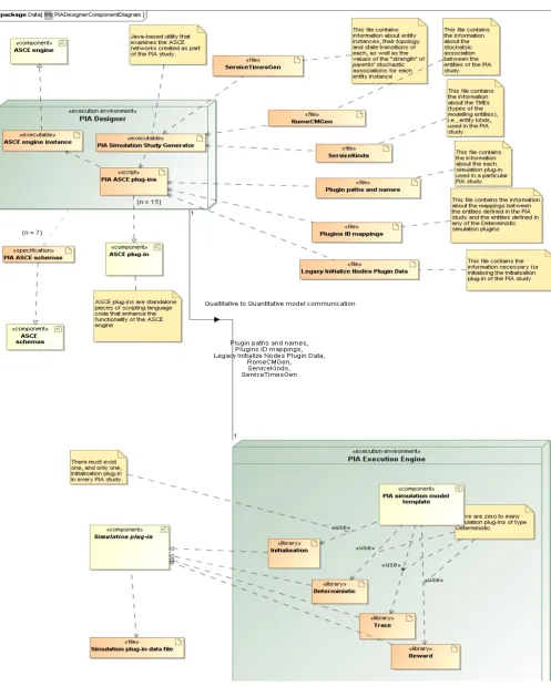
A schematic representation of the PIA Toolkit architecture is given in Figure 5, as a UML Component diagram. The component diagram displays the software execution environment of the whole PIA toolkit. It models the software with concrete elements in the physical world that are the result of a development process and reveals software configuration issues through dependency relationships.

PIA Designer consists of the following components:

● An instance of the ASCE tool executable,

● 15 PIA ASCE plug-ins which implement the functionally necessary for the qualitative PIA. The plug-ins are implemented using JavaScript programming language, with the exception of one of them, PIA_InterServiceLinks.xml, which is implemented using VBscript language.

The plugins enable the PIA analyst to create the PIA model views, each one of which uses a PIA ASCE schema as its underlying notation. The ASCE plug-in referred to as

PIA_SimulationPluginsConfigurator.xml is used for the creation of a subset of the files used

as inputs to the PIA execution environment – these files are used for the configuration of the simulation plug-ins used in the simulation model. There are 3 such files: Plugin paths and names, Legacy Initialize Nodes Plugin Data, and Plugins ID mappings.

● Seven PIA ASCE schema files which are used as the underlying notations for the various PIA model views (ASCE networks):

● PIA.xml, PIA_InterCIPN.xml, PIA_InterCISA.xml, PIA_IntraSA.xml, PIA_Project.xml, PIA_SimulationPlugins.xml, PIA_StateTransitions.xml.

These ASCE schemas are general–purpose. They are to be used in an arbitrary PIA study. In addition to these 7 schemas, PIA assumes that a separate schema for Intra-PN view is created for each service modelled in a particular PIA study. In one of the case-studies used throughout the PIA:FARA project, we have created 2 such schemas: PIA_PowerPN.xml and PIA_TelcoPN.xml, which are used for graphically representing Power and Telco CI service,

respectively, of the Rome case-study.

● The PIA Simulation Study Generator utility, which examines the ASCE networks created by

the PIA ASCE plug-ins and creates 3 input files necessary for the execution of the PIA simulation: i) ServiceTimesGen file – this file contains the data about the entities used in the

PIA study and the corresponding topology, the data about the state transitions of each entity instance, and the values of the parent scaling factors for each entity instance; ii)

RomeCMGen – this file contains the information about the direction of the stochastic

(28)

of entities it stochastically influences (“children”) is provided; and iii) ServiceKinds – this

file contains the information about the TMEs (types of the modelling entities), i.e., entity kinds, used in the PIA study.

The PIA Execution Engine uses the files generated by the PIA Designer as its inputs. This part of the PIA toolkit includes the following components:

● PIA simulation model template, which is initialised in the specific way for each PIA study. The initialisation data are obtained from the 3 input files generated by the PIA Designer:

ServiceTimesGen, RomeCMGen and ServiceKinds.

● Exactly one simulation plug-in belonging to the Initialisation category. This plug-in implements the initialisation of the PIA simulation model template for a particular PIA study according to the information supplied in the three input files. The data file for the initialisation plug-in contains the absolute path to the directory of the simulation model where the three input files are located.

● (Optional) A set of simulation plug-ins belonging to the other categories. Each of these

plug-ins has a data file associated to it. Also, there is another file specific to the simulation plug-ins belonging to the Deterministic category. The file, titled Plugins ID mappings,

(29)

[image:29.595.90.588.107.728.2]

(30)

3.5 Tool support for the service-level model

In addition to the ASCE plug-ins used for the development of the PIA Designer tool (see Section 3.4), we have implemented a couple of ASCE plug-ins which aid the creation of the model of interacting services (service-level model).

As discussed in Section 2.2.4, the identification of dependencies between CIs lies upon the careful consideration of the relationships between model entities, and a thoughtful process of asking what-if questions and applying scenarios to the model.

Here, the tool and the effort placed in providing the definitions and the service model begin to produce results: assisted by the visualisation of ASCE’s graphical environment, the user can explore dependencies by examining the network and can communicate scenarios and findings with colleagues. In addition, the PIA Toolkit also comes with two ASCE plug-ins that can be used to enhance this investigation. These are discussed in the following sub-sections.

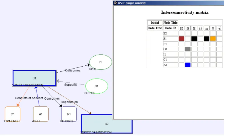
[image:30.595.86.480.397.636.2]

3.5.1 Interconnectivity matrix plug-in

Figure 6 shows a screenshot of the Interconnectivity matrix plugin. The plugin can be used to present in a tabular format the various links between the model entities devised in service-level model. This can be used to improve the visualisation of associations and dependencies between services.

Figure 6: Interconnectivity matrix plug-in

Furthermore, the blank cells in the matrix indicate that there is no dependency recorded between the entities in the corresponding pair. The user can comment on the justification for why there is no dependency between the two entities.

(31)

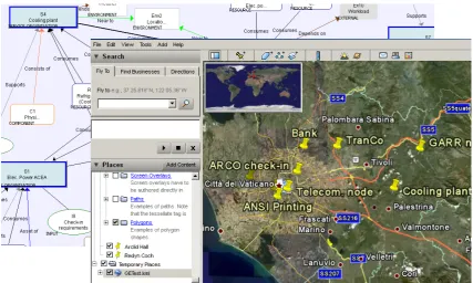
3.5.2 Google Earth plug-in

[image:31.595.84.512.186.442.2]

In order to consider the aspect of geographical dependencies, Geographical Information Systems (GIS) need to be used. Having entered the geographical coordinates for each entity modelled in the ASCE network, invoking the Google Earth plug-in will result in a map being produced which represents nodes in the model and their service status (see Figure 7).

Figure 7: Google Earth plugin

These two plug-ins, along with the ASCE graphical environment, can facilitate the qualitative examination and investigation of dependencies. Once the system has been built, the analyst can begin to ask what-if questions, and reconfigure the model parameters to observe changes in the system behaviour. As discussed in Section 2.2, the information about the system, previous incidents and the threat agents will shape a threat model that can drive this exercise.

4 Conclusions

This report presented the PIA approach and described how the associated toolkit is to be used to carry out a PIA study. This section summarises the benefits of using this approach.

PIA is a lightweight, fairly quick and easy, affordable approach to identifying and analysing interdependencies in complex systems. The analyst, with very low start-up costs, can model the entire system under investigation, starting from a high level of abstraction, and taking a modular approach to model development. With PIA, the analyst will be able to identify, analyse and quantify the risk of interdependency down to a physical component level.

(32)

identify further requirements for specific elements of the system, whilst maintaining a good understanding of the entire system within the wider scope of the models. Given the costs of such modelling, carefully deciding what to model will support making the right decisions in terms of resource allocation, hardware performance requirements and investment overall.

The WP2 of the PIA:FARA project delivered a tool-supported method, along with supporting guidance for CI interdependency analysis. Besides the use of the method on a case study based on the incident near Rome, Italy (see Appendix B), the method has also been applied internally within the project on another case-study which models an SME’s information infrastructure. The case studies were important since they served as a validation for the method and the tools. They also helped the PIA developers to identify the areas of improvement and further

(33)

5 Glossary

Term / abbreviation

Explanation

AFI Abstract Functional Interface API Application Programming Interface

ASCE Assurance and Safety Case Environment, Adelard

http://www.adelard.com/web/hnav/ASCE/index.html

CI Critical Infrastructure

Coupling point A model entity that represents an interface between different CI services Dependency Single direction dependencies of one infrastructure on another

DSBM Detailed Service Behaviour Models GIS Geographical Information Systems IA Interdependency analysis II Information Infrastructure

IRRIIS Integrated Risk Reduction of Information-based Infrastructure Systems LLP Limited Liability Partnership

Möbius A software tool for modelling the behaviour of complex systems, developed by the PERFORM research group from the University of Illinois at Urbana-Champaignwww.mobius.illinois.edu/

PC Personal Computer

PERFORM Performability Engineering Research Group PIA Preliminary Interdependency Analysis

PIA Toolkit A set of software tools to support the PIA method PSTN Public Switched Telephone Network

PVS PVS is a specification language integrated with support tools and a theorem prover. See http://pvs.csl.sri.com

SAN Stochastic association networks are mathematical modelling formalism which provide stochastic extensions to Petri nets and are typically used for performance and dependability evaluation.

SMEs Small-to-Medium Enterprises

State Model entities can have a variety of states that i) describe their different phases of operation (e.g. start-up, operating, shutdown, maintenance), ii) describe their level of operability (e.g. OK, impaired, failed), iii) indicate characteristics of the commodities supplied (e.g. power phase angle for electrical power services). The definition of the possible states/modes that a PIA model entity can occupy is necessary for the identification and analysis of (inter)dependencies between model entities.

State machine A mathematical abstraction which describes the behaviour of model (entity) and is composed of a finite number of states and state transitions.