A numerical investigation into Southern Ocean sea ice using CICE version 4 0

(1)

A numerical investigation into Southern Ocean sea ice

using CICE version 4.0

by

Roger P. Stevens

Master of Philosophy

Bachelor of Engineering

Submitted in fulfilment of the requirements for the Degree of

Doctor of Philosophy in Quantitative Marine Science

(A joint CSIRO and UTAS PhD program in quantitative marine science)

University of Tasmania

(2)

Declarations

I hereby declare that this thesis contains no material which has been accepted for the award of any other degree or diploma in any tertiary institution, and to the best of my knowledge contains no copy or paraphrase of material previously published or written by any other person, except where due reference is made in the text of the thesis.

Signed: ... Roger P. Stevens

Date: ...

Authority of access

This thesis may be available for loan and limited copying in accordance with the Copyright Act 1968.

Signed: ... Roger P. Stevens

(3)

(4)

Acknowledgements

I would like to thank:

My wife Stella. This PhD was one of her many good ideas. She not only put up with my sea ice obsession but supported me in every way during my candidature. Thank you for enabling the best years of my working life, so far.

My supervisors Petra Heil, Kelvin Michael, and Steve Rintoul. Particular thanks go to Petra, who was so generous with her time and full of useful suggestions. Thank you for providing a rich and rewarding student experience.

The Los Alamos National Laboratory for developing CICE4 and making it available.

Neil Adams for supplying the grid, the land mask, and the atmospheric forcing data and for his help in reprocessing and understanding this data.

Simon Marsland for supplying the ocean forcing and for his suggestions concerning model configuration.

National Computing Infrastructure (NCI) for hosting my computations and for help with using their systems. This research was undertaken with the assistance of resources provided at the NCI through the National Computational Merit Allocation Scheme supported by the Australian Government.

Joe Comiso for passive microwave-derived ice concentration data.

National Centers for Environmental Prediction (NCEP) for reanalysis air temperature and wind speed.

National Aeronautics and Space Administration (NASA) for the figure of Antarctica.

My son David O’Donohue and also Simon Wotherspoon for their assistance with statistics.

Also my daughter Kate Stevens, who, when she was only six, created one of the section headings.

(5)

Abstract

(6)

List of Figures

1.1 Antarctic continent . . . 3

2.1 Speedup vs number of CPUs . . . 17

2.2 Effect of the number of ice thickness categories on ice volume and CPU time. . 19

2.3 Ice thickness difference ncat = 5 minus ncat = 1 to 7 . . . 20

2.4 Ice thickness for ncat = 5 . . . 21

2.5 Panantarctic domain . . . 22

2.6 Passive microwave and simulated ice concentration . . . 25

2.7 Variability of passive microwave total ice area . . . 26

2.9 Model sensitivity to mixed layer depth . . . 28

2.10 Model sensitivity to air temperature . . . 29

2.11 Model sensitivity to cloud fraction . . . 30

2.12 Model area sensitivity to ice density . . . 31

2.13 Model volume sensitivity to ice density . . . 32

2.14 Ice parameter steps at changes in grid cell . . . 34

3.1 Fraction of PM total ice area for 1999 without adjustment . . . 38

3.2 1998 to 2008 average of monthly average air temperature . . . 38

3.3 Monthly average air temperature . . . 40

3.4 Difference between seasonal average air temperature PolarLAPS - NCEP . . . 41

3.5 January 1998 average cloud fraction . . . 42

3.6 Monthly average short-wave observations and model . . . 43

3.7 Monthly average long-wave observations and model . . . 44

3.8 Mixed layer depth for 1998 to 2008 . . . 45

3.9 Monthly average wind speeds 1998 to 2008 . . . 46

3.10 Monthly average wind speeds . . . 47

3.11 Difference between seasonal average wind speed PolarLAPS - NCEP . . . 48

4.1 Ice production by month . . . 50

4.2 Congelation ice growth as a function of air temperature and ice thickness . . . 51

4.3 Congelation downward long-wave radiation and surface temperature . . . 51

4.4 Congelation ice growth . . . 52

4.5 Ice thickness 15 July 2007 . . . 53

4.6 Frazil ice growth . . . 54

4.7 Ridging ice thickness growth . . . 55

4.8 Snow-ice growth . . . 56

4.9 Monthly average precipitation example . . . 57

(9)

4.11 Ice decay by type . . . 59

4.12 Basal melt spatial distribution examples . . . 60

4.13 Ice thickness at ice minimum and maximum . . . 61

4.14 1998 to 2008 average of daily total ice area, volume and average thickness . . . 61

4.15 Annual average ice thickness, area, and volume trends . . . 62

4.16 Ice volume anomaly versus ice area anomaly . . . 63

4.17 Ice thickness transects . . . 64

4.18 July zonal distribution of edge speed and ice velocity . . . 65

4.19 Northward expansion of the ice edge and ice velocity . . . 65

4.20 Fraction of zones where northward ice velocity is greater than ice edge expansion rate . . . 66

4.21 IPCC AR4 A1B 2100 simulation as a fraction of the optimized simulation . . . 67

4.22 Ice thickness at ice minimum using IPCC AR4 A1B 2100 projected forcing . . 69

4.23 Ice concentration at ice maximum using IPCC AR4 A1B 2100 projected forcing 70 A.1 Model sensitivity to downward short-wave ratiation in 1998 . . . 92

A.2 Model sensitivity to downward long-wave ratiation in 1998 . . . 92

A.3 Model sensitivity to humidity in 1998 . . . 93

A.4 Model sensitivity to wind strength in 1998 . . . 93

A.5 Model sensitivity to precipitation in 1998 . . . 94

A.6 Model sensitivity to snow thermal conductivity in 1998 . . . 94

A.7 Model sensitivity to snow albedo in 1998 . . . 95

A.8 Model sensitivity to ice albedo in 1998 . . . 96

A.9 Model sensitivity to sea surface salinity in 1998 . . . 97

A.10 Model sensitivity to ocean heat in 1998 . . . 97

A.11 Model sensitivity to ocean drag coefficient in 1998 . . . 98

A.12 Model sensitivity to ocean albedo in 1998 . . . 98

B.1 All VIBs at 2◦ _{longitude resolution in 1998 . . . 100}

D.1 1998 to 2008 average of monthly air temperature January to June . . . 104

D.1 1998 to 2008 average of monthly air temperature July to December . . . 105

E.1 1998–2008 average of monthly wind speed January to June . . . 107

E.1 1998–2008 average of monthly wind speed July to December . . . 108

E.2 1998–2008 average of monthly southerly wind speed January to June . . . 109

E.2 1998–2008 average of monthly southerly wind speed July to December . . . 110

E.3 1998–2008 average of monthly westerly wind speed January to June . . . 111

(10)

List of Tables

2.1 Maximum thickness of ice thickness categories . . . 22

(11)

1. Introduction and Background

1.1 Introduction

Sea ice is subject to dynamic and thermodynamic processes, driven by atmospheric and oceanic forcing and thus may be an indicator of climate change (Lei et al., 2012). It has been proposed that the Earth has left the Holocene and entered a new geologic epoch, the Anthropocene. This new epoch is characterised by climate change due to human activity (Steffen et al., 2007). In order to demonstrate that change is occurring it is necessary to identify which parameters are changing and have methods developed by which they can be measured. Only then can other indicators of climate change be integrated to infer the consequences of climate change on local and global systems. In the northern hemisphere, warming has seen dramatic reductions in sea ice area (Stroeve et al., 2007) and thickness (Rothrock et al., 1999). However, in the southern hemisphere, the signal is less clear. Satellite-based observations have shown that Southern Ocean sea ice extent has actually increased slightly since the 1970s (Zwally et al., 2002; Curran et al., 2003). Estimates of changes in thickness of Southern Ocean sea ice are sparse compared to that of Arctic Ocean sea ice. Therefore, numerical models are likely to increase our understanding of the physical processes driving sea ice mass balance, and help fill gaps where observations are sparse. The research presented here uses the Los Alamos Community Ice CodE version 4 model (CICE4) (Hunke and Lipscomb, 2008) to investigate the physical processes of Southern Ocean sea ice.

1.2 Antarctica

Antarctica was part of the supercontinent Gondwana, along with South America, Africa, India, Australia and New Zealand. About 183 million years ago Gondwana began to break up, and about 40 million years ago Australia separated from Antarctica. Drake Passage opened be-tween South America and the Antarctic Peninsula about 23 million years ago, allowing strong circulation of the ACC to become established, which isolated waters around Antarctica from the warmer waters further north (Stewart, 1990). Antarctica is a large continent of about 13,200,000 km2

(12)

radiation, its large land area and its height means that Antarctica is very cold. The record for the lowest land surface temperature of -89.2◦ _{C was recorded at Vostok Station on 21.07.1983.}

The continental interior has very low precipitation which mostly falls as ice. Ice has accu-mulated to a great depth forming an ice sheet, which flows under gravity towards the coast. Nearer the coast the flow of ice forms into glaciers which can extend into the ocean as floating ice shelves and ice tongues (Rignot and Jacobs, 2002). Ice shelves and ice tongues interact with sea ice in a number of ways. Ice tongues intercept sea ice moving in the Coastal Current (Massom et al., 2003). Thick sea ice forms on the upstream (eastern) side of the glacial ice tongues through dynamic ice growth processes in the convergent conditions encountered there. On the down-stream side the sea ice is thin because the ice that is advected out is not replaced by up-stream sea ice but must be grown thermodynamically so forming a latent heat polynya (Massom et al., 2003). The glacial valleys concentrate the katabatic winds from the higher continent (Adams, 2004) and once unconstrained over the sea ice the winds gain a westward component due to the Coriolis effect. These strong winds quickly remove ice formed within the polynya (Adolphs and Wendler, 1995) exposing the ocean to the cold atmosphere and foster-ing sustained high rates of ice production (Tamura et al., 2008). Polynyas often form near ice shelves for similar reasons. At times continental ice from ice sheets and ice tongues detaches to become icebergs. These are likely to ground in shallow waters and to provide stable anchor points for the formation of land-fast ice. The iceberg/fast ice system also blocks the westward movement of pack ice along the coast and allows the formation of a polynya to the leeward side of the system.

The Antarctic continent is also a source of fresh water to the Southern Ocean. Under the ice sheet there is a fresh water drainage system which eventually discharges to the ocean (Stearns et al., 2008). But there are other sources of fresh water from the Antarctic Continent. Ice shelves melt particularly rapidly near their grounding line (Rignot and Jacobs, 2002). Some of this melt is re-frozen under the shelf itself (Oerter et al., 1992), but some is discharged as freshwater into the surrounding ocean. Adding fresh water lowers the salinity of the ocean and lower salinity in surface waters promotes sea ice growth by raising the temperature at which the ocean freezes. Sea ice production increases the rate of melting of ice shelves at their grounding line (Rignot and Jacobs, 2002). Cold, high salinity water produced under growing sea ice can sink to the depth of the grounding line where it is the source of sensible heat to the ice shelf due to change in freezing temperature caused by higher pressure at depth (Joughin and Alley, 2011).

1.3 The Southern Ocean

The Southern Ocean is the most southerly of Earth’s oceans and extends across all longitude bands. The northern limits can be defined in different ways but a practical oceanographic definition is from the Antarctic Coast to the Antarctic Convergence at about 50-55◦_S

(13)

[image:13.595.87.553.162.632.2]

Figure 1.1: Antarctic continent with major features named. Following Zwally et al. (1983) we have divided the Antarctic sea ice zone into the following sectors: Weddell Sea (60◦_{W –}

20◦_{E), Indian Ocean (20}◦ _{– 90}◦_{E), Pacific Ocean (90}◦ _{– 160}◦_{E ), Ross Sea (160}◦ _{– 220}◦_E),

(14)

its movement. In the northern hemisphere, the Arctic Ocean extends to the Pole, but the Southern Ocean reaches no further south than 77◦_S.

The Southern Ocean surface water temperatures are low, ranging from the ocean freezing temperature (about -1.8◦_{C) to about 10}◦_{C . The surface winds that occur in this region are, on}

average, the strongest to be found anywhere on Earth. Near sea ice maximum, the winds near the ice edge predominantly travel from west to east and drive the ACC in the same direction. While it is not a particularly fast current, i.e. 0.03 to 0.09 m sec−1

(Nybakken et al., 2003) it is wide and extends to great depth so the volume of transported water is large, i.e. 137 Sv (±8) (Rintoul, 2009).

The Southern Ocean contains three continuous, circumpolar fronts. From north to south they are the Subantarctic Front (SAF), the Polar Front (PF), and the Southern ACC Front (Orsi et al., 1995). Near the Antarctic Coast the Coastal Current moves from east to west, driven by easterly winds formed from very cold air that flows off the Antarctic Continent then turns to the west under the influence of the Coriolis effect. Between the Coastal Current and the ACC is a region of upwelling Circumpolar Deep Water (CDW) known as the Antarctic Divergence (AD). Compared to the surface water, the CDW is warm and saline. The surface water, Antarctic Surface Water (AASW), extends with fairly uniform properties from the Antarctic Continent to the Polar Front, and is the water mass which interacts most with sea ice. Near the Antarctic Coast the sea ice moves westward with the prevailing currents and winds. A little further north, sea ice often has a northward component to its trajectory enabling it to cross the AD and turn to the east as it becomes entrained into the ACC and exposed to westerly winds. The AD is not a continuous band within the Southern Ocean. Instead, it is disjointed where large gyres extend far north to connect into the ACC. The largest of these gyres are found in the Weddell and Ross seas. Sea ice within these gyres may advect south in the eastern arm of the gyre and return to travel westward in the Coastal Current. There are smaller gyres as well, for instance in Prydz Bay (centred on 75◦_{E), one in the Indian Ocean}

sector centred on 40◦_{E, and another in the Pacific Ocean sector centred on 110}◦_E.

It is common to subdivide the Southern Ocean into five regions (Zwally et al., 1983) (Fig. 1.1). Sea ice trends may differ in different regions. For instance, the Ross Sea sector has experienced an increase in sea ice area and extent over the past 30 years (Comiso et al., 2011). In the Bellingshausen and Amundsen seas sector the trends are the opposite where sea ice area and extent have declined since the 1970s (Jacobs and Comiso, 1997).

1.4 Sea Ice

Sea ice is an important component of the climate system of the Earth. While most sea ice is frozen ocean water, some sea ice forms by metamorphoses of overlying snow and some forms from other sources. Water ice is an unusual solid in that it is less dense in its solid phase than in its liquid phase. This means that ice formed within the water column will rise towards the surface due to buoyancy forces. When ice formed at the surface is pushed below the waterline by ridging or rafting processes, these buoyancy forces will maintain contact between the upper and lower layers, forming a new thicker ice profile. Sea ice therefore forms a layer separating the ocean from the atmosphere. Sea ice is important to climate because it greatly alters the energy and mass fluxes between ocean and atmosphere.

(15)

wavelengths for snow-free first year ice and ≈0.96 if covered by >0.03 m of snow (Brandt et al., 2005). This compares to the ocean which has a very low albedo of≈0.07 (Brandt et al., 2005; Allison et al., 1993). Once sea ice has formed it reflects back into the atmosphere much of the downward shortwave radiation that would otherwise heat the ocean. This effect tends to maintain the ice cover, i.e. it is a positive feedback. However, ice is a good thermal insulator, especially if covered by dry snow. As the ice grows in thickness, its insulating properties reduce the rate at which ice can grow thermodynamically (Ebert and Curry, 1993).

Sea ice acts as a physical barrier to gas exchange and largely decouples the momentum exchange between ocean and atmosphere (Raphael, 2003). Therefore, the air above sea ice is much drier and colder than air that can interact with the ocean. When moist air moves into the sea ice zone it is likely to form low-level ice cloud, which reduces the amount of shortwave radiation that reaches the sea ice. Atmospheric properties (temperature and humidity) change rapidly over relatively short distances at the ice edge and the instabilities associated with this can promote the formation of cold air mesocyclones (Carleton and Fitch, 1993; McMurdie et al., 1997). These systems subsequently influence the movement of sea ice, and hence the position of the ice edge.

Sea ice exists in many forms. Ice crystals formed within the water column are called frazil ice and they can collect under existing ice or can form a layer of grease ice at an ice-free ocean surface. Grease ice is a mixture of ice crystals and sea water and its physical properties are between those of solid ice and sea water (Smedsrud, 2011). In calm conditions the grease ice fuses into thin sheets of ice called nilas (Allison et al., 1993). If the ocean surface is agitated by waves then the grease ice forms into pancake ice (de la Rosa et al., 2011). Thermodynamic ice growth rates can be large when ice is thin but are slower as thickness increases (Allison, 1979). In the Southern Ocean, ice thicker than ≈0.4 m is usually the result of ridging and rafting of thin ice (Allison and Worby, 1994).

In coastal polynyas, sea ice is constantly being removed to expose open water so polynyas are sites of high frazil ice production (Allison and Worby, 1994; Gow et al., 1987). While the wind is favourable to polynya activity the average ice thickness in the polynya remains low and ice production is high. The Antarctic coastal polynyas are primarily latent heat polynyas with latent heat fluxes of 174 W m−2 _{reported for the Ad´elie Depression compared to transported}

sensible heat fluxes of 30 W m−2

(Williams and Bindoff, 2003). They are called latent heat polynyas because the latent heat of fusion of water to ice largely balances the heat flux from ocean to atmosphere (Adolphs and Wendler, 1995).

While ocean waves can influence how sea ice forms and the distribution of floe sizes, sea ice also affects waves. Shortwave ocean waves are quickly attenuated during their interactions with the ice floes and do not penetrate past the marginal ice zone (Vaughan et al., 2009; Kohout and Meylan, 2008). Longwave ocean waves, on the other hand, can penetrate deep into the pack ice where they can cause large floes to break (Bennetts et al., 2010).

Early in the ice growth season, the ocean is stratified with relatively cold, fresh, surface shelf water overlying warmer, more saline Circumpolar Deep Water (CDW). In the process of ice crystal formation the salt in the ocean water is expelled, forming a network of brine pockets in the sea ice, which may connect into brine channels. The formation of interconnecting brine channels is temperature-dependent (Golden, 2001; Golden et al., 2007) with cold ice (<-5◦_C)

(16)

is incorporated into the surface mixed layer, any heat it contains can come into contact with the sea ice above. This may slow ice growth (Allison, 1979). On the other hand, ice growth may continue in shallow waters near the coast, where the full water column may be cooled to freezing point, especially in the high ice production regions of the coastal polynyas. High salinity shelf water from these regions spills over the shelf break, entraining the overlying Lower CDW as it sinks, becoming Antarctic Bottom Water (AABW). AABW ventilates the deep ocean and is an important driver of the meridional overturning circulation (Orsi et al., 1999).

Sea ice is also biologically important. On the small scale, plankton may become incorpo-rated into sea ice as it freezes, and live in the brine channels. The rafting process will often introduce ocean water with its plankton into the layer separating the ice layers. Plankton may also be carried into the interface between the ice and the snow during flooding, for example, due to snow loading. Plankton becomes biologically active in spring and is released into the surface layer of the ocean as the sea ice first becomes porous and then melts. The plankton finds itself in optimal conditions for growth and multiplication due to the long hours of sun-light, surface water stratification (Williams et al., 2011a) and the injection of micronutrients such as iron that have accumulated on the sea ice (Lannuzel et al., 2008). The plankton bloom that follows the retreating ice edge supplies food for primary consumers such as krill that can swarm in their millions. Krill, in turn, are food for many predators including fish, squid, penguins, seals, and baleen whales.

The Weddell seal’s life history is tied to fast ice and during the height of the last interglacial its distribution was reduced to the deep embayments, where sea ice survived (Younger, 2010). Similarly, Emperor Penguins breed on fast ice and depend on it surviving until the chicks have fledged. So in years when the fast ice breaks-up early, which can be associated with a reduced sea ice barrier, breeding success is low (Massom et al., 2009). Other penguins such as the Adélie breed on land but feed in sea ice and their breeding success depends on having sea ice near to their breeding colonies. There appears to be an optimum amount of sea ice for successful breeding of Adélie penguins but the relationship is complex with important factors being the timing of the occurrence of sea ice and the type of sea ice. For instance, if the penguins have to cross a large distance of land fast sea ice to feed when they are in the “guard phase” of the breeding cycle then breeding success is low (Emmerson and Southwell, 2008). During the last 26 years there has been a decrease in sea ice extent west of the Antarctic Peninsula and Adélie and chinstrap penguins on the South Orkney Islands have suffered reductions in numbers while less ice adapted species like gentoo penguins have increased their population (Forcada et al., 2006).

1.5 The known, the unknown, and contributions of this

research

1.5.1 Research questions

This section addresses the research questions examined in this thesis and attempts to relate published research to each topic. It begins with the three research questions, followed by a little background and then proceeds to each question in turn.

(17)

2. In the current climate state, how much do thermodynamic and dynamic processes con-tribute to the position of the sea ice edge around the Antarctic?

3. High-latitude signature of climate change is strongest in the atmospheric circulation. What changes in Southern Ocean sea ice can be expected from the projections of future climate?

1.5.2 General background

While there are some historical records of Antarctic sea ice (i.e. de la Mare, 1997), the study of Antarctic sea ice has benefitted greatly from the deployment of satellites with passive microwave sensors. Scanning Multichannel Microwave Radiometer, Special Sensor Microwave Imager, Advanced Microwave Scanning Radiometer based observations are available from 1979 onwards. These sensors have been deployed on polar orbiting satellites leaving a polar-centred area about a 2.4◦ _{wide area void of data. A number of algorithms have been developed}

to derive sea ice concentrations from measurements of microwave brightness temperatures. Inter-comparisons of the algorithms show that these give slightly different estimates of ice area and extent (Comiso and Parkinson, 2008). Various datasets have been derived from ice concentration including sea ice extent, sea ice area, and sea ice duration (Bjørgo et al., 1997; Parkinson et al., 1999; Cavalieri et al., 2003; Cavalieri and Parkinson, 2008).

The Arctic and Antarctic display very different trends over the interval of satellite-based passive microwave observations. Over the last 33 years, sea ice extent in the Arctic has experienced a dramatic decline of up to -5% per decade, and averaging -3.4% per decade (Comiso and Nishio, 2008). In the Antarctic, sea ice extent has actually increased slightly, at a rate of about +1% per decade (Zwally et al., 2002; Cavalieri and Parkinson, 2008; Comiso and Nishio, 2008). Circum-Antarctic average extent does not tell the full story because it integrates over regions where there have been significant decreases as well as over regions where there have been significant increases. For instance, the Bellingshausen-Amundsen seas sector exhibits a decline of almost 10% in the 20 years after 1979 but the Ross Sea sector had an almost 7% increase in the same period (Zwally et al., 2002).

The increasing trend in sea ice in the Ross Sea and the decreasing trend in the Bellingshausen-Amundsen seas are primarily associated with changes in the Southern Annular Mode (SAM) (Comiso et al., 2011). Annular modes exist in both hemispheres and are large scale patterns of climate variability which exist because of internal atmospheric dynamics in the middle lat-itudes. They are characterized by latitudinal changes in the position of air masses and in winds at 55–60◦ _{and 30–35}◦_{. While the mechanism for producing the large-scale atmospheric}

pressure and wind patterns is well understood the fundamentals of low-frequency variability (annular modes) are still being determined (Jin, 2009). Positive SAM is associated with an increased probability of low sea level pressure in the Bellingshausen-Amundsen seas sector (Stammerjohn et al., 2008). The atmospheric circulation around these low pressure systems produces winds with a northerly component west of the Antarctic Peninsula and a southerly flow over the Ross Sea. Northerly winds bring warm air into the sea ice region, therefore suppressing thermodynamic sea ice production as well as driving sea ice towards the coast. On the other hand, the southerly winds over the Ross Sea bring cold continental air into the sea ice region promoting thermodynamic ice growth and advecting ice north.

(18)

multi-year ice (Maslanik et al., 2007). The Arctic sea ice appears to become more like that of the Antarctic, where most of it is first-year ice, because less ice survives summer to become second-year ice. There are more measurements of sea ice thickness in the Arctic than in the Antarctic, including estimates obtained from upward-looking sonar on submarines (Tucker III et al., 1998). Falling well short of such a data set, the Southern Ocean sea ice thickness is documented in the ASPeCt database which estimates ice thickness from ship-based visual observations (Worby et al., 2008). Additionally, passive microwave measurements of brightness/temperature can be used to estimate ice thickness in latent heat polynyas for ice thicknesses less than 0.2 m (Tamura et al., 2007). Satellite- or aircraft-based measurements of ice thickness are becoming available (Farrell et al., 2009). Lidar-based systems can be used to measure freeboard and then estimate ice thickness using the Archimedes principle plus some assumptions about ice and snow density and snow loading (V´arnai and Cahalan, 2007; Xie et al., 2010; Farrell et al., 2011). Radar has also been used to estimate freeboard (Giles et al., 2008). Such techniques work better in the Arctic where snow thickness is generally low but in the Southern Ocean the higher snow loading makes the estimates less reliable (Kwok, 2010). As a consequence less is known about trends in sea ice thickness in the Southern Ocean. Numerical sea ice models can be used to compute ice thickness in regions or at times when observations are missing or sparse. For example, the Louvain-la-Neuve sea ice model (LIM) has simulated Southern Ocean sea ice on a 2◦_×₂◦ _{grid (Vancoppenolle et al., 2009). With a view to contributing to a}

regional sea ice forecasting system, this research uses a higher resolution 0.25◦_×_0.25◦ _grid.

1.5.3 Research question 1

“What is the relationship between variability in sea ice volume and that of sea ice area?” Ice area is well established from satellite-based passive microwave measurements since the late 1970’s (Comiso and Zwally, 1984). Ice thickness is less well constrained by measurements and therefore ice volume cannot be calculated with the same degree of certainty.

The surface temperature measured in satellite-based passive microwave observations can be used to estimate thin ice (<0.2m) (Tamura et al., 2007). This is very useful for mapping sea ice production in polynyas (Tamura et al., 2008; Tamura and Ohshima, 2011) but is less use in the pack generally where ice thicknesses are mostly greater than 0.2m.

There is also the ship-based estimated of snow and ice thickness (and concentration) in the ASPeCt data set (Worby et al., 2008). While this data set is very useful it is rather sparse in space and time compared to the daily passive microwave estimates of total ice area.

Dynamic ice growth in thickness is very common with rafting of thin ice and ridging of thicker ice (Worby et al., 1996). Dynamic ice thickening causes changes in surface roughness which are also reflected in the roughness of overlying snow, and this can be used to estimate ice thickness (Toyota et al., 2011b).

(19)

1.5.4 Research question 2

“In the current climate state, how much do thermodynamic and dynamic processes contribute to the position of the sea ice edge around the Antarctic?”

In the Southern Ocean there is normally a gradient in ice concentration from high values within the pack to zero in the open ocean to the north. This region of rapidly decreasing ice concentration is called the marginal ice zone (MIZ) and is associated with high gradients of environmental variables (Andreas et al., 1984). However, there are anomalous conditions where the ice edge is quite compact (Massom et al., 2008). Defining the ice edge can be done in different ways depending on the needs and the situation. Since passive microwave receivers have been flying in satellites in the late 1970’s the conventional definition has been 15% ice concentration because this is close to the limit that these instruments can reliably detect sea ice (Comiso and Zwally, 1984). The accuracy of detecting the ice edge from space varies with season such that the accuracy is good in winter but there are confounding effects in summer which reduce accuracy (Worby and Comiso, 2004). The low ice concentration in the MIZ means that ice-ice interactions are rare and the floes are in a free drift condition (Lepp¨aranta, 2005).

The ice edge advance and retreat correlates with the position of the -2.16◦_{C surface}

tem-perature isotherm (Comiso and Zwally, 1984). During the ice growth season the total ice area increases, with high concentration ice just south of the ice edge. During the ice decay season, ice area is lost by a southward movement of the ice edge plus a decrease in ice concentration within the pack (Comiso and Zwally, 1984). In many zones in spring, thin ice, such as that in coastal polynyas, will melt and form an inner ice edge that moves northward to meet the southward moving ice edge “aice 2008.gif”.

For the time interval 1992-2001 there is a strong correlation between the ice drift velocity and the geostrophic wind velocity, i.e. R2

≈0.7 in the Weddell and Indian Ocean sectors (maximum 0.9 in the Amundsen Sea), while correlations between the northward expansion rate of the ice edge and the northward ice velocity are lower, i.e. R2

≈0.5 in the Weddell Sea sector and R2

≈0.4 in the Indian Ocean sector (maximum 0.7 in the Amundsen Sea) (Kimura, 2007). Kimura (2007) also found that, during the ice growth season, there were two distinct relationships for the short-term northward expansion rate of the ice edge to northward ice velocity: one where the ice edge is advancing and another when it was retreating. While advancing the northward expansion rate of the ice edge is greater than the northward ice velocity and while retreating the northward expansion rate of the ice edge is very similar to the northward ice velocity.

(20)

(Wadhams et al., 1987). At other zones ice advection determines the location of the ice edge. An extreme example is at 85◦_{E where wind and currents combine to produce a tongue-like}

extension of the ice edge (Rintoul et al., 2008).

The location of the ice edge in spring and summer is more difficult to determine from satellites due to higher water content in the atmosphere and because of wet ice and snow during the melt (Worby and Comiso, 2004). Kimura (2007) restricted his analysis to sea ice concentrations between 40-50% and to the months of May to October to define their ice edge. This was necessary to obtain ice motion from satellite observations. The analysis in this research uses a lower range of ice concentrations for calculating ice drift speeds, i.e. 1-30%, but the seasons were limited to middle autumn to early summer (April to December) because of the complexity of the ice edge in many zones from January to March. This research quantifies the thermodynamic and dynamic contributions to the maintenance of the location of the ice edge. This is achieved by comparing the northward expansion rate of the ice edge to the northward ice velocity at the ice edge. This is done at 1◦ _{intervals around the Southern Ocean and for}

the months when there is circum-Antarctic sea ice, i.e. April to December.

1.5.5 Research question 3

“High-latitude signature of climate change is strongest in the atmospheric circulation. What changes in Southern Ocean sea ice can be expected from the projections of future climate?”

Surface atmospheric temperatures have risen over land and oceans contributing to a global average rise of 0.74◦ _{in the 100 year time interval 1906 to 2005 with the land warming at}

about twice the rate of the oceans (0.27◦ _decade−1 _{for land and 0.13}◦ _decade−1 _{for oceans)}

(Solomon et al., 2007) chapter 3. At high latitudes the changes have been greater due polar amplification such that the Arctic has warmed two to four times faster than the global average (Screen et al., 2012). The southern hemisphere also has a “hot spot” of surface warming in the Antarctic Peninsula even if warming trends over continental Antarctica are in line with the global mean increase (Vaughan et al., 2003).

The warming climate has seen changes in atmospheric circulation (Corti et al., 1999). In mid and high latitudes this is mostly seen in the Annular Mode, which accounts for the largest part of climate variability in these regions (Jones et al., 2009). The Southern Annular Mode (SAM) has tended toward more positive values (Stammerjohn et al., 2008). Positive SAM is associated with lower air pressures over Antarctica and a pole-ward intensification of the westerly winds at about 50◦_{S latitude (Ho et al., 2011). Positive SAM is associated with}

warming over the Antarctic Peninsula (Thompson and Solomon, 2002).

The most commonly used and accepted set of greenhouse gas emissions scenarios, known as the SRES emissions scenarios, comes from the IPCC. These were last updated in 2000 in the Special Report on Emissions Scenarios (SRES). They are now named the SRES emissions scenarios (Nakicenovic and Swart, 2000). The SRES emissions scenarios are divided into six families: A1FI, A2, A1B, B2, A1T and B1. The families are based on future technological and societal changes, such as population growth, and not just on a high, medium and low scale of carbon emissions.

(21)

subgroups based technology: A1FI is fossil fuel intensive; A1T focuses on non-fossil energy sources; A1B has balanced set of technologies which does not rely too greatly on any particular energy source. A1B assumes that all the technologies will have similar rates of improvement in supply and end use technologies. The A1B scenario is usedas the basis of calculating adjustments that were applied to existing forcing for warm climate simulations. Economic growh and energy usage do seem to be rising rapidly, there is some evidence of new technologies being introduced but it remains to be seen if a more equitable distribution of weath will eventuate.

Projections for the Southern Ocean from climate model simulations include increases in air temperature, surface air pressure, precipitation, cloud fraction, downward long-wave radiation, air humidity, and wind speeds. The values in the next five paragraphs are taken from the IPCC Fourth Assessment Report chapter 10 (Solomon et al., 2007).

Anthropogenic green house gasses that find their way into the atmosphere cause warming of the troposphere. Estimated global average increase of air temperature by 2100 for the A1B scenario are 1.7–3.4◦_{C, compared to those of the time interval 1980 to 1999. The oceans are}

also warming but at a slower rate because they have higher thermal inertia.

Cloud fraction is important in determining the amount of shortwave radiation reaching the surface and in the amount of long-wave radiation prevented from escaping into space. The IPCC models predict an increase of 1-2% in high level cloud fraction in the sea ice zone for the A1B scenario. This reduces the model mean short-wave radiation flux reaching the surface by 0.13 ±0.11 W m−2 _{and increases the long-wave radiation by 3.8}_±_{0.33 W m}−2_.

Global average precipitation is projected to increase by more than 3% by 2100 for the A1B scenario. In the Southern Ocean the rate of precipitation is projected to increase by +0.2 mm day−1 _{for this scenario compared to 1980-1999. The global mean precipitation increases in all}

scenarios because of the increased water-holding capacity of the atmosphere (Douville et al., 2002).

Sea level air pressure is projected to increase over the subtropics and decrease over the higher latitudes. This is associated with an expansion of the Hadley Circulation and a pole-ward shift in storm tracks. The models consistently show a positive trend in the Southern Annular Mode (SAM). Some models show an increase in cyclones and an intensification in the southern hemisphere westerly winds (Lynch et al., 2006). Associated with the higher frequency of strong storms is an increase in extreme wave height.

Some models produce a poleward shift in the surface westerly winds, accompanied by a southerly movement of the core of the Antarctic Circumpolar Current (Fyfe and Saenko, 2005; Gupta et al., 2009) but in other models the ACC moves very little (Graham et al., 2012). Some models show an increase in the strength of the ACC, associated with the stronger surface westerly winds (Fyfe and Saenko, 2005; Gupta et al., 2009), but in eddy-resolving models stronger winds produce an intensified eddy field rather than an increase in ACC volume transport (Hogg et al., 2007).

Since the 1970s there has been a small but significant increase of 0.97% decade−1

(22)

The thesis is divided into seven chapters:

1. “Introduction” which is this chapter, provides an introduction and overview of Antarc-tica, the Southern Ocean, and sea ice. It also gives some background to topics relating to the research questions.

2. “Model and Methods” which describes CICE4 and other software developed for this project. This chapter also describes the tuning of the model and the sensitivity of the model to the fields used for tuning.

3. “Forcing” which examines the external forcing used.

4. “Results” which describes the experiments used to address the research questions and the results of these experiments.

5. “Discussion” which discusses the results and how they relate to other published work.

6. “Conclusions” which gathers the main results and states how the research questions were addressed.

(23)

2. Model and Methods

2.1 CICE4

2.1.1 Introduction to CICE4

The numerical model CICE4 (Community Ice CodE) was used to investigate the three research questions. CICE4 simulates total ice area and volume which are used in an examination of how area and volume vary for the years 1998 to 2008. CICE4 also simulates ice velocity obtained from the dynamics of the model. The northward component of ice velocity was compared to the northward speed of the ice edge to assess the importance of ice advection in maintaining the position of the ice edge. Finally, predictions can be made about the future of Southern Ocean sea ice by running the model with forcing fields compatible with climate projections for the year 2100.

This section describes CICE4 as it was configured for this research. CICE4 was developed by the Los Alamos National Laboratory as part of the Climate, Ocean and Sea Ice Modeling Project. Many individuals and groups contributed to the model but the principal developers are Elizabeth Hunke and William Lipscomb. CICE4 is written in Fortran90 and can be run on parallel computers using Message-Passing Interface (MPI) as it was for this research. Details on running CICE4 in parallel can be found in Section 2.2. CICE4 can utilize files in NetCDF (Network Common Data Form) for I/O and this is how it was configured for this research. CICE4 is designed to be run coupled to ocean and atmospheric models but can also be run standalone as was done for this research. Our standalone configuration used forcing from the regional atmospheric model Polar Limited Area Prediction Systems (PolarLAPS) and the ocean global ocean model Australian Climate Ocean Model (AusCOM).

2.1.2 Thermodynamic and dynamic processes in CICE4

CICE4 represents sea ice as a thickness distribution. The surface of the ocean is divided into grid cells and each grid cell contains an ice thickness distribution, which has zero thickness for open water. The ice thickness distribution can change by the thermodynamic processes of ice growth and decay or by ice advection and dynamic growth. The equation used to calculate changes in the ice thickness distribution is equation 3 in Thorndike et al. (1975):

∂g

∂t =− ▽.(gu)− ∂

(24)

where u is the horizontal velocity,f is the rate of thermodynamic ice growth, ψ is the ridging redistribution function, and g is the ice thickness distribution function. The first term on the right hand side of the equation 2.1 is the horizontal transport of ice. The second is the change in thickness due to thermodynamic growth or melt. The third term is the dynamic ice growth from ridging and rafting.

The right hand elements of equation 2.1 are evaluated in sequence starting with the ther-modynamic growth/decay then ice advection by horizontal transport and ending with dynamic growth through ridging. The continuous ice thickness distribution is approximated by ice thick-ness categories (refer Section 2.4). Each thickthick-ness category is treated as a uniform column of thickness hin = vin/ain where vin is the volume of ice in category n and ain is the fractional

ice area in this category. Each column is divided into Ni layers, where Ni = 4 by default.

The fractional area of all ice categories is given byai =

Pn

1 ain and the ice area of each grid

cell can be obtained by multiplying the fractional area by the grid cell area. Total ice area is the sum of the area of ice in each grid cell. Similarly, the volume of ice in each grid cell is the sum of the volume of ice in each category and the sum of the volume of all grid cells gives the total ice volume. Total ice area and total ice volume are used for the first research question examining how ice area and volume covary.

Snow is known to have an important influence on sea ice processes. Snow is treated in a similar manner to ice in that the snow thickness is calculated by hsn = vsn/ain where vsn is

the snow volume for ice category n. Snow can have multiple layers Ns, but the model default

is Ns = 1. Snow is not created within CICE4 as ice is but is supplied externally to the model

as precipitation forcing.

CICE4 calculates the grid scale ice velocities and moves ice from one grid cell to an adjacent one by a process of incremental remapping in 2-dimensional horizontal space (Dukowicz and Baumgardner, 2000). The ice is then re-arranged within the ice thickness distribution of each grid cell by another process of incremental remapping within thickness space (Lipscomb, 2001). These processes preserve ice volume and other state variables such as snow volume, internal ice and snow energy, surface temperature, and volume-weighted mean ice age. It is the ice velocity

u that is used to investigate research question two into the contribution of ice dynamics in the form of advection to the maintenance of the position of the ice edge.

Growth or decay at the ice-ocean interface and decay at the ice-snow-atmosphere interface is determined by the energy balance at these surfaces (Maykut and Untersteiner, 1971). Energy fluxes at the top surface are long-wave radiation down from the atmosphere and clouds, short-wave radiation down, reflected short-short-wave radiation up, long-short-wave radiation up from thermal emission, sensible and latent heat exchange with the surface atmosphere, heat conduction within the ice and snow, and penetrating radiation which is absorbed within the ice and snow (Maykut and Untersteiner, 1971). Below the freezing point of fresh water the energy balance of the top surface is maintained by changes to the surface temperature and hence the upward long-wave radiation flux. At the freezing point of fresh water it is the latent heat of melting that balances excess energy fluxes into the ice. Moisture from the air can condense onto the top surface but most mass is added to the top via snow fall. Precipitation falling as rain is assumed to run-off quickly into the ocean.

(25)

growth or melt conditions the heat balance at the bottom surface is maintained by the latent heat of fusion. The heat conduction into the submerged sides of the floe can cause lateral melt. Arctic lateral melt rates have been estimated using the difference between sea surface temperature and the temperature of ice at the bottom of the floe Maykut and Perovich (1987) equation 12 :

Mr =m1△T_wm2 (2.2)

wherem1 = 1.6×10− 6

m s−1 ◦_C−1.36_{, and}_m₂ _{= 1}_._{36. Lateral melt rate can be combined with}

floe diameter to give the fraction of ice that melts laterally (Steele, 1992):

rside= Mr∗dt∗π

α∗φf loe

(2.3)

where α is a constant which for the Arctic Ocean has a value 0.66 (Rothrock and Thorndike, 1984), and φf loe = 300 m is the average floe diameter.

CICE4 models sea ice as a plastic medium which reacts to low stresses like a nonlinear viscous compressible fluid. The rheology that describes this behaviour is called viscous-plastic (Hibler III, 1979). CICE4 uses a modification of this rheology called elastic-viscous-plastic rheology (Hunke and Dukowicz, 1997). At time scales associated with wind forcing the elastic-viscous-plastic rheology reduces to the elastic-viscous-plastic rheology but at shorter time scales the adjustment process is via the computationally more efficient mechanism of elastic waves.

The internal ice stress tensor can be obtained from the viscous-plastic constitutive law, which relates ice stress to strain rate. Internal ice stress is used in the two dimensional momentum equation (Hibler III, 1979):

m∂u

∂t =▽.σ+−→τa+−→τw−ˆk×mfu−mg▽Ho (2.4)

where m is the combined mass per unit area of ice and snow, u is the horizontal velocity,

t is time, σ is internal stress,−→τa is wind stress,−→τw is ocean stress, the fourth term on the right

is the Coriolis stress, and the fifth term is the stress due to the sea surface slope (where g is the acceleration due to gravity).

A discrete version of the momentum equation is used by the model to calculate ice velocity. The ice velocity is then used to estimate dynamic ice growth in high ice concentration regions of convergence. To ensure that closing of open water is more likely than ridging CICE4 uses a weighting function (Thorndike et al., 1975). The weighting function gives preference for the ridging of thin ice rather than to thick ice. Sufficient ridging will occur so that the ice area in the grid cell does not exceed the area of the grid cell.

2.1.3 Snow-ice in CICE4

(26)

the sea surface. A snow loading sufficient to depress the snow-ice interface to sea surface is obtained when the ratio of snow thickness to ice thickness is equal to the ratio of snow density to ice density. Both snow density and ice density are constants in CICE4 with values ρsnow = 300

kg m3

and ρice = 917 kg m

3

giving a maximum snow thickness to ice thickness ratio of 0.33. Volume and energy is then transferred from the snow layer to the top ice layer.

2.2 Domain Decomposition and Speedup

2.2.1 Introduction

This section describes the domain decomposition and speed-up experiments. The “panantarc-tic” domain, containing 330×330 grid cells, can be subdivided into blocks. Each compute processor can work on one or more blocks. For rectangular blocks it is better to have more grid cells in the y-direction (less processors) than the x-direction (more processors). However, with a square grid many of the configuration options have square blocks. The number of processors and the number of blocks is set in the compile scripts. The shape and options for optimization are set in the name list.

2.2.2 Domain Decomposition

In parallel computing a speed-up in the time it takes to complete solving a problem (the elapsed time) is obtained by dividing the problem into discrete “chunks” and distributing these to the computing tasks available. In the case of simulating Southern Ocean sea ice the chunks are parts of the “panantarcitc” domain and are called “blocks”. Each block contains grid cells representing land, ocean only, or ocean and sea ice. Making the blocks smaller increases the number of computing tasks that can be applied to solving the problem but it also increases the communications overhead because each block has to communicate its results to its neighbours. Increasing the communications overhead increases the computational resources needed to solve the problem (CPU time). The domain blocks should be chosen to ensure that each computing task has a similar amount of work to do and will finish in about the same time. This is called load balancing. In the case of simulations of Southern Ocean sea ice the aim is to have about the same number of sea ice containing grid cells in each block.

The less the blocks have to communicate with each other the more efficiently the model runs. Square blocks have smaller boundaries for the number of grid cells they contain, compared to thin rectangles for example, and thus minimize communications between blocks. Each block has a set of “ghost cells” around the edge which contain the values from adjacent blocks. MPI maintains the ghost cells with the current values from the adjacent blocks by passing values each time step.

There are two useful ways to decompose the domain and this is done by setting the processor shape:

• slender (slenderX1 or slenderX2)

• square (square-ice)

(27)

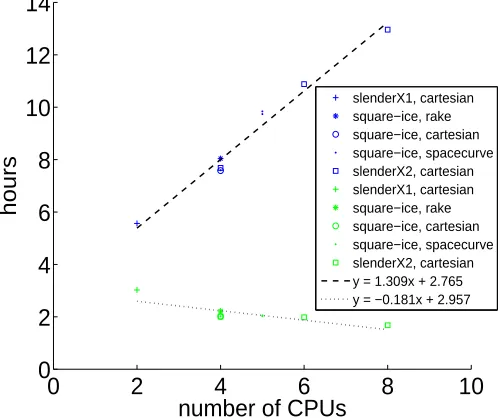
Ocean and the other end in the Southern Ocean. This is not a very useful configuration on the curvilinear “panantarctic” grid because some blocks near the edge will contain only ocean. Other blocks near the middle will contain a lot more land cells than blocks between the edge and the middle of the domain. “slenderX2” is also designed for a rectilinear grid creating two sets of strip like blocks which meet at the equator so each block will have only one end in the Arctic or Southern oceans. “square-ice” divides the domain into blocks of squares and is almost equivalent in computing effort to “slenderX2” when there are 4 equal blocks each running on one processor (Fig. 2.1). Therefore “square-ice” is used in this research.

0 2 4 6 8 10

0 2 4 6 8 10 12 14

number of CPUs

hours

[image:27.595.191.441.236.445.2]

slenderX1, cartesian square−ice, rake square−ice, cartesian square−ice, spacecurve slenderX2, cartesian slenderX1, cartesian square−ice, rake square−ice, cartesian square−ice, spacecurve slenderX2, cartesian y = 1.309x + 2.765 y = −0.181x + 2.957

Figure 2.1: Run time as a function of the number of CPUs

2.2.3 Speed-up

In order to determine the optimum configuration for domain decomposition that gives de-creased elapsed time while not requiring excessive computing resources, experiments were undertaken with various methods for domain decomposition. The CPU and elapsed time are measured for similar runs with 2, 4, 5, 6 and 8 CPUs. With an increasing number of CPUs, the elapse time (telapse) decreases at a rate of:

telapse=−0.181x+ 2.957 (2.5)

However, the CPU time (tCP U) increases at the much faster rate of:

tCP U = 1.309x+ 2.765 (2.6)

(28)

The combinations of “square-ice” or “slenderX2” has elapsed times for 4 CPUs that are almost the same as for 5 and 6 CPUs (Fig. 2.1). Thus there is no elapsed time benefit to running with 5 or 6 CPUs.

2.3 Model Spin-up

The model can be started from two states: a) zero ice; or b) 2 m of ice south of 60◦_{S. For the}

default ice thickness categories either option was successful. However, for the optimized ice thickness categories (Table 2.1 right hand column) it was better to start from the “zero ice” option. To obtain a stable model condition for the start of experiments beginning in January 1998, the model is run for five years using 1998 forcing. The simulation rapidly converges on a stable value, because very little Antarctic sea ice survives the spring and summer to become second-year ice. So the model almost resets itself every year. The total ice area converges rapidly towards a stable state, i.e. on 31 December the total ice area of cycle 5 is less than 0.002% different from that of cycle 4. Average ice concentration changes by only -0.00005% between cycle 4 and 5. The largest differences in ice concentration are found in the central Weddell Sea, which is one of the locations where ice survives throughout the summer. Average ice thickness changes by 0.17% between cycle 4 and 5. The largest differences in ice thickness are found in the small embayments around the coast.

2.4 Ice Thickness Categories

Experiments are undertaken to determine the optimum set of ice thickness categories. There are two parts to this, the number of categories and the maximum thickness for the categories.

2.4.1 Number of Ice Thickness Categories

In this research five ice thickness categories were used for all runs other than those investi-gating the impact of ice thickness categories on model performance. Five thickness categories are sufficient to allow patterns of variable thickness to develop. Adding more ice thickness categories generally increased the ice thickness and hence ice volume, but it also increased the computing effort needed to run the model. However, the increase in total ice volume when the number of ice thickness categories is increased from 5 to 7 is small.

The number of ice thickness categories, denoted in CICE4 as “ncat”, was varied between 1 and 7. The following simulation fields are examined:

• ice thickness distribution in space

• total ice area

• total ice volume

• model run time

(29)

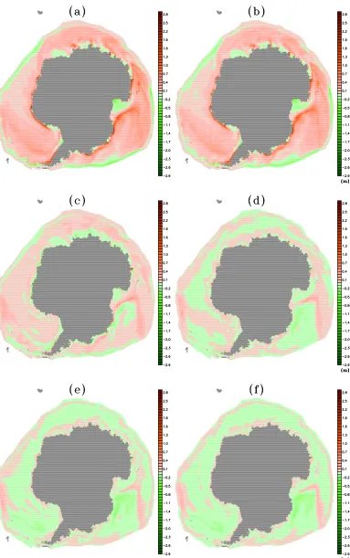
distribution, lacking regions of extremely thick ice (Fig. 2.3a and 2.3b). For three ice thickness categories, most of the thick ice and thickness features are present but subdued (Fig. 2.3c). For four and five ice thickness categories, the thickness of the thickest ice increases (Fig. 2.3d and 2.4). There is very little change in increasing from five to seven ice thickness categories (Fig. 2.3e and 2.3f), i.e. seven categories increases average ice thickness by 0.01 m compared to five categories, and the maximum difference in ice thickness is 0.8 m thicker. The maximum value is located on the up-stream side of a coastal protrusion. The differences are smaller in the central pack ice, i.e. mostly less than ±0.2 m.

The number of ice thickness categories has a small effect on total ice area, i.e. increasing from 5 to 7 categories increases the annual average total ice area by 2.7×104

km2

or 0.26%. The increase in total ice area occurred between the middle of November and the end of April, with a peak of 2×105

km2

in early January. For the rest of the year, increasing the number of ice categories decreases the total ice area with a maximum decrease of 2.8×104

km2

in late September.

Progressing from three to seven ice thickness categories produces a small increase in ice volume from 9.51×1012

km3

to 10.18×1012

km3

(Fig. 2.2a). There is a step from two to three categories, i.e. ncat=2 produces an ice volume of 7.80×1012

km3

. Increasing ncat from 5 to 7 produces a maximum increase in ice volume in mid November and a minimum increase in mid March with an annual average increase of 1 ×1011

km3

or 1%. For ncat >5 there is little improvement in spatial distribution of ice thickness and, in going from 5 to 7 ice thickness categories, there was only a 0.46% increase in total ice volume. Therefore, the model was run with ncat = 5 for this research and presented, from this point on, in this thesis.

1 2 3 4 5 6 7

7 7.5 8 8.5 9 9.5 10 10.5

number of ice thickness categories

annual average ice volume [x10

1

2 km 3 ]

(a)

1 2 3 4 5 6 7

1 2 3 4 5 6 7 8 9

number of ice thickness categories

hours CPU time elapsed time y=0.748x+3.487 y=0.189x+0.899

(b)

(30)

[image:30.595.132.515.100.711.2]

(31)

[image:31.595.94.550.96.545.2]

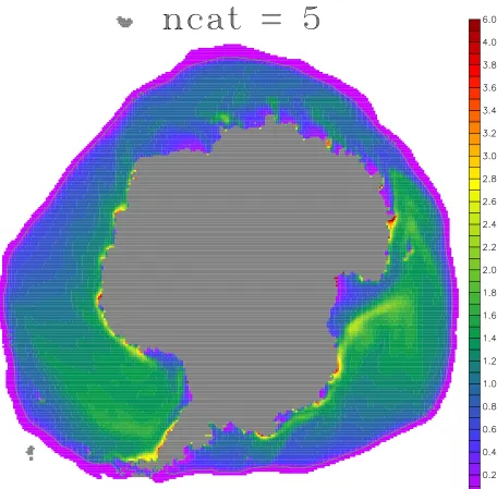
Figure 2.4: Ice thickness on 8 October 1998 for where number of categories = 5. Also shown is the 15% ice concentration contour (green) and land mask (grey). Ice thickness scale is bi-linear with 4–6 m at a lower resolution.

2.4.2 Maximum Thickness of Categories

(32)

of convergence associated with weather systems (Heil et al., 1998).

maximum thickness [m] category default set modified set

[image:32.595.222.418.124.245.2]

n=0 0.000 0.000 n=1 0.645 0.125 n=2 1.391 0.354 n=3 2.470 1.000 n=4 4.567 2.000 n=5 9.334 6.000

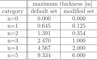
Table 2.1: Maximum thicknesses for the default ice thickness categories and modified to opti-mize for Antarctic sea ice for this research.

[image:32.595.127.520.325.718.2]

(33)

Configuring CICE4 ice thickness categories for the Antarctic involves having thinner maxi-mum thickness for each category. A number of experiments have been undertaken with various maximum category thicknesses. Increasing the maximum thickness of the thinner categories, while keeping the thickest category unchanged, produced larger total ice area in summer and early autumn. For the rest of the year the total ice area is slightly less. Increasing the max-imum thickness of the thickest ice category, while keeping the lower category thicknesses the same, has very little effect on total ice area. For ncat = 5 increasing the maximum thickness of the thin categories, while keeping the thickest category the same, produces a larger ice volume in mid and late summer but slightly less for the rest of the year. Increasing the maximum thickness of the thickest category while keeping the lowest category the same produces greater ice volume with a maximum in late October or early November. But the magnitude of the changes are small, i.e. less than 3% for area and less than 2% for volume.

2.5 The configuration of CICE4 for this Research

Unless specified CICE4 was run with the default parameters as specified in the user manual (Hunke and Lipscomb, 2008). For this project CICE4 is run as a moderately high resolution, regional model over the Southern Ocean. It is run on the “panantarctic” grid which includes all the sea ice regions around Antarctica (Fig. 2.5). The grid contains 330×330 grid cells and has the point of longitudinal convergence, which would normally be at the South Pole, displaced to the equator. Moving the longitudinal convergence is not important for the operation of CICE4 because it does no computation over the Antarctic Continent but it is for PolarLAPS which is used to model Antarctic weather. There is also a 90◦_{, anticlockwise rotation of the}

grid so the prime meridian is horizontal and to the left. The dimensions of the grid cells vary over the domain but is ∼27 km. In the x-direction the size of the grid cell is 27.80 km and in the y-direction cells vary from 18.00 to 28.00 km (Fig. 2.5).

The model’s land mask was based on the Mosaic Of Antarctica (MOA) (URL: http://nsidc.org/data/moa/).

Modifications include the addition of landfast sea ice and sub-Antarctic islands. Islands have an effect when they interact with sea ice. Landfast sea ice acts very like land as far as pack ice is concerned. The landfast ice anchored by grounded icebergs is considered as land and included in the land mask (Fig. 2.5).

The time step of the model can be varied, but for this study it is one hour. This means that the spatial resolution is sufficiently large to avoid numerical instabilities associated with the ice dynamical calculations (Courant et al., 1928). The model is run standalone with forcing from the high resolution atmospheric model PolarLAPS and from the ocean general circulation model AusCOM.

The depth of the ocean’s mixed layer has a strong influence on the amount of ice produced during the time interval when daily change in total ice area is positive. On average this is from the second half of February to the second half of September or from about day-of-year (DoY) 49 to 263. The model is modified to read in a hourly mixed layer depth (MLD).

(34)

MLD and so air temperature is used to tune the model at this time of year. An adjustment value was read every time step and added to air temperatures over the model domain (Section 3.4.1). The adjustment value was added to each forcing grid cell value.

The model is modified to calculate a time-varying value for deep ocean heat entering the mixed layer based on Antarctic observations near Mawson Station (Allison, 1979). The deep ocean heat flux is greatest when ice production is greatest (25.60 W m−2_{) early in the ice}

growth season (DoY 90) and has another, lesser peak value (6.97 W m−2

) in October (DoY 278). Outside the interval of DoY 86 to 334 the deep ocean heat was set to zero. In reality the deep ocean heat would vary in space as well as time but having a time-varying value is an improvement over the static value that is the default for the model. The annual average is about 4.5 W m−2 _{which is low compared to 16 W m}−2 _{measured in the Weddell Sea (Gordon}

and Huber, 1990).

Running the model with a forced Sea Surface Temperature (SST) produced unrealistic spatial sea ice distributions. The solution to this is to use the slab representation of the ocean, internal to the model and thus allow natural, two-way interactions between ice and ocean. In this configuration the ocean is the mixed layer and is 1-dimensional in each grid cell. That is, water and energy are not moved between grid cells, even though the model incorporates ocean currents. These currents interact with sea ice only and do not move water within or between grid cells.

Lastly, the model is modified to calculate the surface downward radiation internally to the model (Sections 3.4.3 for short-wave and 3.4.4 for long-wave).

2.5.1 Sample simulations

This section presents simulations from a typical year compared to observations. A number of model fields can be used to do this comparison, including total ice area, concentration, and thickness.

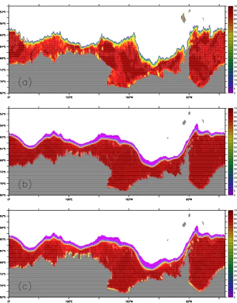
Simulated ice concentrations (Fig. 2.6b) are compared to those estimated from the bright-ness temperature at microwave wavelengths (Fig. 2.6a). In July ice is growing and air temper-atures are low so any open water within the pack is quickly frozen over with thin ice. Therefore the simulated ice concentration appears much higher than passive microwave estimates. The simulation could be more accurate because the algorithms used to analyse the passive mi-crowave measurements have difficulty distinguishing thin ice from open water (Comiso and Steffen, 2001). When the thinnest simulated ice category is subtracted from the total ice con-centration more structure appears within the pack (Fig. 2.6c). Despite this improvement the simulated pack ice has a much more uniform ice concentration than those derived from passive microwave.

(35)

[image:35.595.82.550.89.689.2]

Figure 2.6: Ice concentration on 15 July 2007: (a) passive microwave; (b) total simulated; (c) total - concentration of thinnest ice category. Also shown is the land mask (grey).

(36)

wider in the simulation and the simulated ice edge is smoothed. The algorithms used to analyse the passive microwave data cannot reliably detect sea ice at concentrations much below 15% while the model is able to identify ice down to very low concentrations. The relative smoothness of the simulated ice edge is more difficult to explain but is most likely caused by the averaging the model does over the grid cell.

Total ice area can easily be calculated by summing the product of the ice concentration within a grid cell by the area of the grid cell. There is a very good agreement1

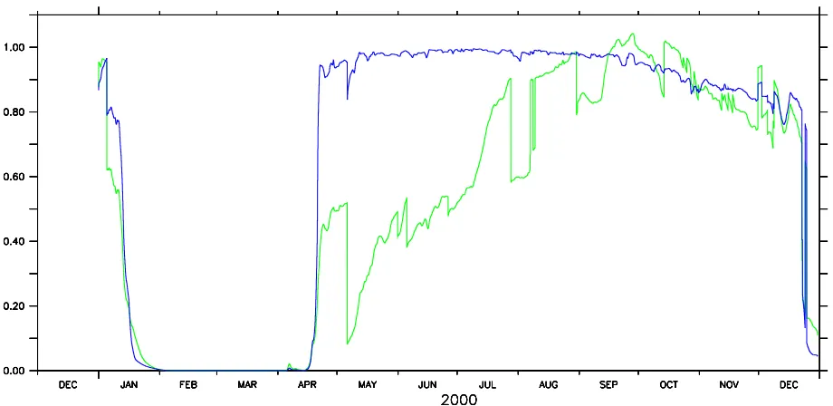
between the simulated total ice area and that derived from passive microwave (Fig. 2.8a). This is not sur-prising because the model was tuned to achieve this. However, the passive microwave-derived total ice area exhibits higher frequency variability. This can be highlighted by subtracting the simulated total ice area from the passive microwave-derive values (Fig. 2.7). From day 131 to day 285 there appears to be minor peaks and troughs superimposed on major peaks and troughs. The average period of the major variations is about 26 days (25.7 for peaks and 25.8 for troughs) and that of the minor variations is about 6.5 days. Synoptic weather systems have durations in the range of 6.5 days and this could be an explanation of the minor variations. The moon orbits the earth every 27.3 days (sidereal month) so a lunar cause of the major variations is not out of the question. However, 25.7 days is less close to the synodic month which is about 29.5 days which makes a lunar connection seem less certain.

Jan Feb Mar Apr May Jun Jul Aug Sep Oct Nov Dec

−0.6 −0.4 −0.2 0 0.2 0.4 0.6 0.8 1 1.2

difference in daily total ice area [x10

6 km

2 ]

passive microwace − simulated

Figure 2.7: Variability over time intervals of days to a month revealed by subtracting the simulated total ice area from that derived from passive microwave averaged for 1998 to 2003.

Simulated total ice area and total ice volume are available in the log files. Average ice thickness can be calculated by dividing total ice volume by total ice area. Average ice thickness varies with season, from thinnest in early autumn and thickest in late summer (Fig. 2.8b). The explanation of this somewhat counter-intuitive behaviour is found in section 4.3.

1

plotting the simulated against the passive microwave has a slope of 1.00 and an R2

of 0.995 with the

(37)

19980 1999 2000 2001 2002 2003 2004 2005 2006 2007 2008 5

10 15

Area [x10

6 km

2]

(a) Modelled total ice area (black) and passive microwave-derived total ice area (red).

0 0.6 1.2 1.8

Thickness [m]

1998 1999 2000 2001 2002 2003 2004 2005 2006 2007 2008 0

6 12 18

Volume (dashed) [x10

3 km

3 ]

Area (solid) [x10

6 km

2 ]

[image:37.595.100.800.80.366.2]

(b) Simulated average ice thickness (black), average ice area (solid red) and average ice volume (dashed red).

Figure 2.8: Eleven year simulation time series (1998–2008)

A numerical investigation into Southern Ocean sea ice using CICE version 4 0