Protocol for soil functionality assessment in vineyards

SOiL functionality in

degraded areas within

organic VinEyards

European research project

2015-2018

PROTOCOLS FOR

ACKNOWLEDGMENTS

Financial support for this project was provided by funding bodies within the FP7 ERA-Net CORE

Organic Plus, and with co-funds from the European Commission.

Authors

Edoardo Costantini (CREA, Italy) Simone Priori (CREA, Italy) Sylvia Landi (CREA, Italy)

Alessandra Lagomarsino (CREA, Italy) Maurizio Castaldi (CREA, Italy)

Brice Giffard (Bordeaux Sciences Agro, France) Emma Fulchin (ADERA Vitinnov, France) Javier Tardaguila (University of La Rioja, Spain)

Hans-Josef Schroers (Agricultural Institute of Slovenia, Slovenia)

Anna Martensson (Swedish University of Agricultural Sciences, Sweden) Semih Tangolar (University of Cukurova, Turkey)

Erhan Akca (Alata Horticultural Research Station, Turkey)

Summary

Summary ... 2

Overview ... 3

About ReSolVe project ... 3

How to use this guide ... 3

Introduction ... 4

Soil functions and functionality ... 4

Why optimal soil functionality in vineyard is important ... 4

Part I: Soil monitoring ... 5

Methodological sheet n°1: soil profile description and sampling... 6

Methodological sheet n°2: bulk density assessment ... 8

Methodological sheet n°3: water retention curve and available water capacity assessment ... 10

Methodological sheet n°4: standard physical and chemical soil analysis ... 12

Part II: Monitoring of soil ecosystem service provision and providers ... 19

Methodological sheet n°5: organic matter breakdown assessment using Tea-Bag Index ... 20

Methodological sheet n°6: earthworms monitoring ... 22

Methodological sheet n°7: enzymatic activities assessment ... 23

Methodological sheet n°8: assessment of soil respiration, microbial biomass and communities ... 25

Methodological sheet n°9: soil mesofauna using Berlese-Tullgren extractors... 28

Methodological sheet n°10: nematodes monitoring ... 30

Part III: Soil rhizosphere monitoring ... 32

Methodological sheet n°11: assessment of communities and pure culture isolation of root- or rhizosphere-associated fungi and bacteria ... 33

Methodological sheet n°12: direct assessment of mycorrhizal infections in root samples ... 36

Part IV: Grapevine monitoring ... 37

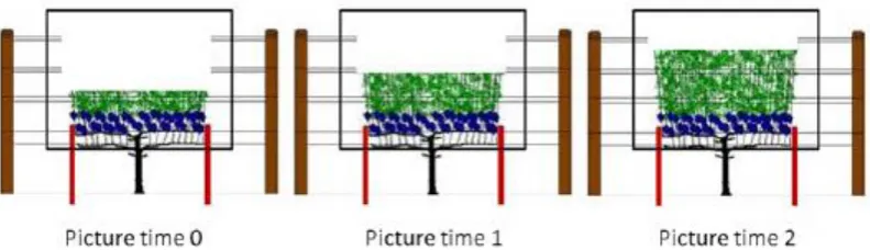
Methodological sheet n°13: grapevine vegetative growth assessment using machine vision ... 38

Methodological sheet n°14: grapevine water status assessment ... 40

Methodological sheet n°15: grape yield assessment ... 42

Methodological sheet n°16: grape composition assessment ... 43

Overview

About ReSolVe project

The ReSolVe project aims at testing the effects of selected agronomic strategies for restoring optimal soil functionality in degraded areas within organic vineyard. The term "degraded areas within vineyard" means areas having been reduced vine growth, disease resistance, grape yield and quality. These areas can have lost their soil functionality because of either an improper land preparation, or an excessive loss of soil organic matter and nutrients, erosion and/or compaction, metal accumulation. The project individuated the main causes of the soil functionality loss and tested different organic recovering methods, such as adding compost, adoption of green manure with different species, and dry mulching. The effects of these techniques were evaluated through the monitoring of various components and consequences of soil functionality:

- soil physical, chemical and hydrological properties, such as organic matter content, soil nitrogen and water availability;

- soil and root-zone biodiversity and biological activity: abundance and diversity of microorganisms, microfauna and earthworms, enzymatic activities, organic matter turnover, mycorrhizae;

- grapevine behaviour as a response to soil status: plant water stress, plant phenology, grape yield and quality.

More information about the project can be found on www.resolve-organic.eu.

How to use this guide

The purpose of this guideline is to describe the methods used during ReSolVe project for soil functionality assessment, so they can be implemented in similar studies.

A brief introduction first underlines what are the main functions of soil and why maintaining an optimal soil functionality is particularly of major interest in viticulture.

Then the different protocols selected for ReSolVe project and this guideline are presented according to the following classification:

- Part I: assessment of soil physical and chemical features;

- Part II: assessment of soil biological features (ecosystem service provision and providers); - Part III: assessment of rhizosphere biological features;

- Part IV: assessment of grapevine quantitative and qualitative indicators reflecting soil functionality. In each part, global objectives of the monitoring are explained (what is it used for, in which cases…) and the

parameters to evaluate are listed with their corresponding methodological sheet. In these sheets, instructions and information are given about:

- Materials needed to perform the sampling and the measurement - Sampling procedure

- Analysis procedure

- Possible interpretations and conclusions that can be drawn (value and meaning of the results, indication of reference values when existing, potential limit of the protocol)

- Bibliographic references related to the method described

Introduction

Soil functions and functionality

The soil functions concept emerged during the early 1970’s (Glenk et al., 2012) and was adopted for the

development of the EU Soil Framework Directive with seven key soil functions (European Commission, 2006):

• Biomass production, including in agriculture and forestry

• Storing, filtering and transforming nutrients, substances and water

• Biodiversity pool such as habitats, species and genes

• Physical and cultural environment for humans and human activities

• Source of raw materials

• Acting as carbon pool (store and sink)

• Archive of geological and archaeological heritage.

Dominati et al. (2010) suggested the following roles of soils in the provision of services:

• Fertility role

• Filter and reservoir role

• Structural role (i.e. physical support)

• Climate regulation role

• Biodiversity conservation role

• Resource role.

These correspond roughly to the soil functions as presented by the European Commission (2006) and are overlapping with the general concept of an Ecosystem Service. One aspect that might be added is the increasing awareness of cultural services.

Soil functionality is the degree of soil function extend and can be quantitatively or qualitatively evaluated.

Soil function describes what the soil does. Soil functions are: (1) sustaining biological activity, diversity, and productivity; (2) regulating and partitioning water and solute flow; (3) filtering and buffering, degrading, immobilizing, and detoxifying organic and inorganic materials, including industrial and municipal by-products and atmospheric deposition; (4) storing and cycling nutrients and other elements within the

earth’s biosphere; and (5) providing support of socioeconomic structures and protection for archeological

treasures associated with human habitation. (Seybold et al, 1998).

Why optimal soil functionality in vineyard is important

Part I: Soil monitoring

Objectives

In experimental projects linked to soil, the differences of soil traits between different areas of the fields should be investigated to characterize them and their spatial variability. In this purpose, profile digging allow to obtain detailed information about soil physical, chemical and hydrological properties, grapevine roots description, and to sample for further laboratory analyses (Methodological sheet n°1: soil profile description and sampling).

Analyses to perform

The samples collected in the profiles can be analyzed for the following standard laboratory analysis:

Analysed parameter Description of the analysis method

Bulk density assessment Methodological sheet n°2

Water retention curve and available water capacity

assessment Methodological sheet n°3

Standard physical and chemical analysis:

- Texture

- pH-water

- Electrical conductivity (EC)

- Total carbonates (equivalent CaCO3)

- Total organic carbon content (TOC)

- Total nitrogen content (TN)

- Cation exchange capacity (CEC) and exchangeable bases (K, Na, Mg, Ca)

Methodological sheet n°4

Some of these parameters can then be monitored throughout the experimentation to evaluate their

Methodological sheet n°1: soil profile description and sampling

Materials needed

▪ Excavator ▪ Measuring tape

▪ Labels to indicate the code of the profile ▪ Camera

▪ Small short-handled shovel ▪ Plastic bags

▪ Marker pen

▪ Net with regular squares (15x15cm)

When and where to dig a profile and sample

The soil profile description should be done in spring or early summer, when the soil is slightly humid. To describe the grapevine root distribution, the profile should be dug around 30 cm far from the vine row.

How to proceed

The soil profile might by dug at a minimum depth of 1 m. A vertical surface of the profile must be cleaned and leveled to take a picture. On the picture, a measuring tape and a sign with the code of the profile should be clearly visible. The soil profile has to be described following the methods of FAO (Figure 1): www.fao.org/3/a-a0541e.pdf.

For grapevine roots description, a lateral wall of the profile should be dug at about 10 cm far from the vine row. The surface of the wall must be roughly cleaned from large clods and stones. A net with regular squares (15x15 cm in size) must be fastened to the profile wall under the vine row.

For each horizon, fine and coarse roots per square meter should be counted. Fine (feeder) roots: < 2 mm. Coarse roots: > 2 mm.

Soil sampling for laboratory analyses. Undisturbed samples of each soil horizon should be collected in a bag with code. The amount of soil collected for each sample should be around 500 g. In case you have several profiles in the same plot, you can select only few benchmark profiles representative of the different areas of the field where to sample if appropriate.

Soil samples should be dry at a maximum temperature of 40 °C.

Figure 1. The process of soil description, classification and suitability evaluation, as indicated by FAO (Jahn et al., 2006)

Possible interpretations and conclusions

Since the vineyard soils are usually deep cultivated before vines plantation, the soil horizons are usually mixed and disturbed. For this reason, the individuation of genetic horizons and pedogenetic features are not always easy. The most important features to check in detail during soil profile description in vineyard are the following:

- Presence of limiting horizons: one or more horizons that limit grapevine rooting can be observed in the profile. The rooting obstacle could be due to compaction, poor aeration and/or waterlogging, very high coarse fragments fraction (> 50-60%), very high content of calcium carbonate, high salinity, nutrient lack or imbalance. If the limiting horizon is deeper than 80-100 cm, usually it does not have negative effects on grapevine growth, but if it is shallower than 70-80 cm can create serious troubles for grapevine nutrition.

- Discontinuities: in vineyard soils, discontinuities are quite common and they are often due to soil truncation and/or accumulation because of the land levelling or erosion.

- Soil internal drainage: soil with slow drainage and temporary waterlogging is characterized by redoximorphic mottles, which are spots or blotches of greyish (reducing) and/or yellowish-reddish (oxidizing) colour. Higher is the abundancy of greyish mottles, longer is the waterlogging period during the year. In addition, reducing conditions of the soil can be also characterized by black iron-manganese concretions.

- Soil structure: it is the natural organization of soil particles into discrete soil units (aggregates or peds) that result from pedogenic processes. The aggregates are separated from each other by pores or voids. Compaction, scarce organic matter and biological activity can contribute to a scarce structure of the soil. The vine roots can have difficulty to develop in horizons with weak structure or massive.

References

Methodological sheet n°2: bulk density assessment

Materials needed

For field work (sampling)

▪ Hammer-driven double-cylinder sampler or metal cylinders with sharpened edge of known volume

▪ Hammer ▪ Wood block

▪ Straight-edged knife ▪ Small short-handled shovel ▪ Plastic bags

▪ Labels ▪ Marker pen

For laboratory work (analysis) ▪ Oven (105°C)

▪ Electronic balance, 0.01g sensitivity ▪ 2-mm sieve

When, where and how to sample

Soil bulk density (Db) is the mass of dry soil per unit of bulk volume, including the void space (Blake and Hartge, 1986). Bulk density is not an invariant characteristic for a given soil. Changes in soil volume due to changes in water content modify bulk density, particularly in swelling soils. Soil mass remains fixed, but the volume of soil may change as water content changes. For this reason, undisturbed soil samples for bulk density determination by the core method (Blake and Hartge, 1986) should be taken when the soil moisture content is near field capacity.

Basically, the core method consists in collecting, drying and weighing a soil sample of known volume. To do this, clean off the pit face or the field surface, and drive the double-cylinder sampler (Figure 2) into the soil; then, carefully remove the inner cylinder to preserve the sample volume. If a hammer-driven double-cylinder sampler is not available, a metal double-cylinder (ring) with sharpened edge of known volume may be driven into the soil using a hammer and a block of wood.

Extract the cylinder from the sampler, remove excess soil from the bottom using the knife, and transfer the soil sample in a plastic sealable bag. Properly label each sample to show basic information, e.g., project, site, date, plot, depth, and horizon. Collect at least three 100 cm3 _{volume samples from each soil horizon}

(or at 0-10 and 10-30-cm depth) to be able to quantify the variability of the system.

Where the soil is too loose (e.g., sandy soil), or skeleton is abundant and preclude the use of core samplers, to allow core sampling it is advisable the adoption of the excavation method (Grossman and Reinsch, 2002). The excavation method involves digging out a small hole, then oven drying at 105°C and weighing the excavated soil. The volume of the excavation is determined by lining the hole with plastic film and filling it completely with a measured volume of water (or sand, or silicon beads).

How to perform the analysis in laboratory

The dry bulk density (Db) is determined according to the core method (Blake and Hartge, 1986). Undisturbed soil samples are oven-dried at 105°C to constant weight.

In order to correct the Db data for the presence of stones, the quantity of material >2 mm in diameter is determined by wet sieving. Each dry sample is washed on the 2-mm sieve; the material that remained on the sieve is collected and oven-dried at 105°C to constant weight.

Bulk density is calculated as the mass of dry, coarse fragment-free soil per volume of the excavated soil, where volume is also calculated on a coarse fragment-free basis. Below is reported the formula used to calculate soil Db, reported to the nearest 0.01 g cm−3_.

Db = Mass of fine material (g) / Volume of fine material(cm3₎

Possible interpretations and conclusions

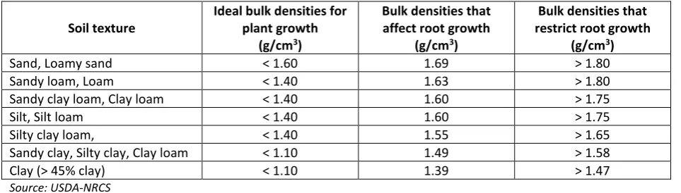
High bulk density values are indicators of low porosity and strong compaction of the soil, aspects that adversely affect water retention capacity, root growth (Table 1) and movements of oxygen and water through the soil. As a consequence, soil compaction causes yield and vegetation cover reduction. By impairing water infiltration, compaction also causes the increase of runoff volume and soil erosion in sloping fields, and the occurrence of flooding in flat areas.

References

BLAKE G.R., HARTGE K.H. (1986). Bulk density. In: A. Klute (ed.) Methods of soil analysis. Part 1, Physical and mineralogical methods, 2nd ed., Agron. Monogr. 9. ASA and SSSA, Madison, WI, pp: 363-375.

GROSSMAN R.B., REINSCH T.G. (2002). Bulk density and linear extensibility. In: J.H. Dane and G.C. Topp (eds.) Methods of soil analysis, Part 4. Physical methods. Soil Sci. Am. Book Series No. 5. ASA and SSSA, Madison, WI., pp. 201–228. USDA-NRCS. Soil Bulk Density / Moisture / Aeration – Soil Quality Kit. Guides for Educators. https://www.nrcs.usda.gov/Internet/FSE_DOCUMENTS/nrcs142p2_053260.pdf

Annex

Table 1. General relationship of soil bulk density to root growth based on soil texture

Soil texture

Ideal bulk densities for plant growth

(g/cm3₎

Bulk densities that affect root growth

(g/cm3₎

Bulk densities that restrict root growth

(g/cm3₎

Sand, Loamy sand < 1.60 1.69 > 1.80

Sandy loam, Loam < 1.40 1.63 > 1.80

Sandy clay loam, Clay loam < 1.40 1.60 > 1.75

Silt, Silt loam < 1.40 1.60 > 1.75

Silty clay loam, < 1.40 1.55 > 1.65

Sandy clay, Silty clay, Clay loam < 1.10 1.49 > 1.58

Clay (> 45% clay) < 1.10 1.39 > 1.47

Methodological sheet n°3: water retention curve and available water capacity

assessment

Materials needed

For field work (sampling)

▪ Metal cylinders (rings) with sharpened edge of known volume (70 mm diameter, 30 mm height) and plastic lids

▪ Hammer ▪ Wood block

▪ Straight-edged knife ▪ Small short-handled shovel ▪ Plastic bags

▪ Marker pen

For laboratory work (analysis) ▪ Sand box

▪ Pressure plate extractors ▪ Porous ceramic plates ▪ Compressor (20 bars) ▪ Pressure regulation system

▪ Electronic balance, 0.01-g sensitivity ▪ 2-mm sieve

▪ Oven (105°C)

When, where and how to sample

Soil samples are taken at 0-10 and 10-30 cm depth at the beginning and the end of the trial period. The samplings are always carried out during the Spring months, with soil moisture content near field capacity. Undisturbed soil samples are taken at each soil horizon during soil profiles description using metal cylinders (70 mm diameter, 30 mm height) with a sharpened edge. Cylinders are hammer-driven into the soil at the 0-10 and 10-30 cm depth and carefully removed with a shovel taking care to preserve soil structure and avoid compaction. The soil extending beyond each end of the cylinder was trimmed with a straight-edged knife, and the ring closed with a plastic lid. Three samples per plot and depth are taken at each sampling date.

How to perform the analysis in laboratory

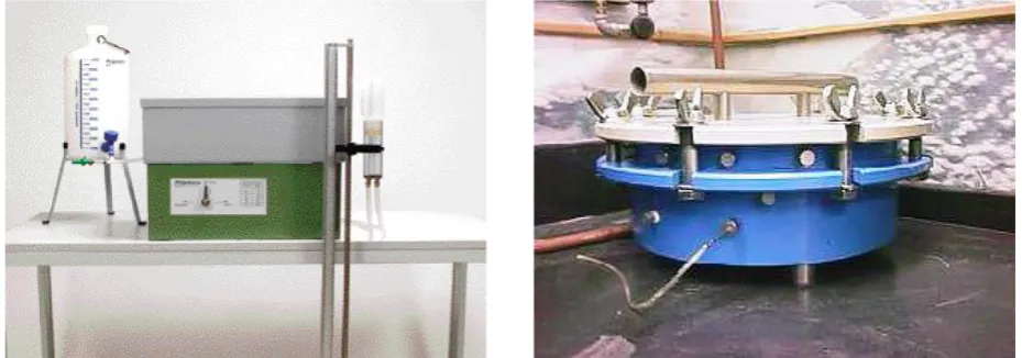
Soil water retention curve is determined by sand box and pressure plate apparatus (Figure 3) on the undisturbed soil samples collected in the experimental vineyards.

Figure 3. Sand box (left) and pressure plate extractor (right)

In the pressure plate extractor method, positive pressure is applied to the air phase of soil samples. The water phase is in contact with atmospheric pressure via a fine-pored porous plate, over which the soil samples are drained (Dane and Hopmans, 2002).

container and secure lid. Apply the proper gauged air pressure. When water ceases to discharge from outflow tube, sample is at equilibrium. Remove the rings and record the weight.

Water content is measured at the 0 (saturation), -6, -10, -33, -600 and -1500 kPa matric potential.

The water content at 0 (saturation), -6 and -10 kPa matric potential is measured on sand box (Clement, 1966), whereas further three retention measurements at the matric potentials of -33, -600 and -1,500 kPa are determined by means of pressure plate extractors (Klute, 1986). The moisture content at each matric potential is then expressed as percentage by weight of the dry soil (d).

The retention data at field capacity (FC) (-10 kPa) and wilting point (WP) (-1,500 kPa) were used to determine the available water capacity (AWC = FC-WP) (Table 2).

On the same soil samples, at the end of the analysis, soil bulk density was determined according to Blake and Hartge (1986), removing by wet sieving the contribution of skeletal (material >2 mm) and plant roots, which particle density was assumed equal to 2.65 and 0.70 g cm-3, respectively. The bulk density values were then used to convert the gravimetric water content (d) data on a volumetric basis (v) by applying the equation (1) (Gardner, 1986).

w d v

BD





 =

(1) where w is the density of water.

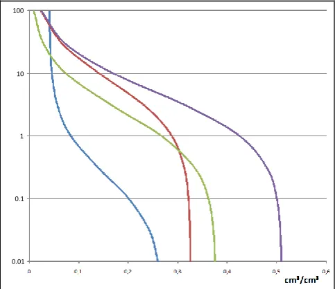
Actually, such a procedure was required to run RETC software (van Genuchten, 1980), employed to determine the retention parameters of soil retention curve (Figure 4), by fitting measured water contents.

Table 2. Matching table for evaluation of the Available Water Capacity (AWC).

Class Values (% on volume basis) Very low < 5

Low 5 - 10

Moderate 10 - 15

High 15 - 20

Very high > 20

10 100

1

0.1

0.01 10 100

1

0.1

0.01

Figure 4. Example of soil water retention curves

References

CLEMENT C.R. (1966). A simple and reliable tension table. European Journal of Soil Science 17(1),133-135.

DANE J.H., HOPMANS J.W. (2002). Water retention and storage: laboratory. In: Methods of Soil Analysis. Part 4- Physical Methods (J.H. Dane & G.C. Topp eds), Soil Science Society of America, Madison, WI, pp. 675-720.

Methodological sheet n°4: standard physical and chemical soil analysis

Materials needed

For field work (sampling) ▪ Shovel

▪ Auger ▪ Plastic bags ▪ Marker pen ▪ Meter

For sample preparation in laboratory ▪ 2-mm sieve

▪ 0.250-mm sieve

▪ Electronic balance, 0.01-g sensitivity ▪ Oven (105°C)

▪ Distilled water

▪ Dispersing solution (containing 2 g of sodium hexametaphosphate/L) ▪ Hydrogen peroxide (H2O2) 30% vol.

▪ Pipettes 25 cm3 _capacity

▪ Cylinders - 500 cm3

▪ Hand stirrer

▪ Common laboratory equipment

Additional specific materials are indicated for each parameter hereafter.

When, where and how to sample

Samples can be collected either in soil profiles at each horizon or in the first 30 cm of soil for a more regular monitoring (especially for total organic carbon, total nitrogen and pH).

In this last case, each experimental plot or modality should be monitored during the main vine phenological phases (budburst, berry formation, pre-veraison, post-veraison) and sampled with a shovel in three randomly selected points at two depths 0-10 and 10-30 cm. The samples from the three sampling points are then mixed thoroughly in a bag with a code to provide a single composite sample.

How to perform the analysis in laboratory

Analysis standard procedures will be performed according to the World Reference Base for Soil Resources classification system (IUSS Working Group WRB, 2014). Full descriptions of the procedures can be found in Procedures for soil analysis (Van Reeuwijk, 2002) and the USDA Soil Survey Laboratory Methods Manual (Burt, 2004).

COMMON SAMPLE PREPARATION

Before analysis, soil samples must be air-dried or, alternatively, oven-dried at a maximum of 30°C. The fine earth fraction should be obtained by sieving the dry sample through a 2 mm sieve. Clods not passing through the sieve should be crushed (not ground) and sieved again. To this aim, a variety of manual or mechanical implements may be used. Gravel, rock fragments, etc. not passing through the sieve are collected and set aside.

TEXTURE (PARTICLE-SIZE) ANALYSIS

Soil texture refers to the relative size distribution of the primary particles in a soil. Particle size, using the USDA classification scheme, is divided into three major size classifications: sand (2.0-0.05 mm), silt (0.05-0.002 mm), and clay (< (0.05-0.002 mm) (Gee and Bauder,1986).

that are widely accepted as standard methods for particle-size analysis (Gee and Bauder, 1986). The procedures are applied to the fine earth (< 2 mm) fraction only.

Materials needed ▪ 2-mm sieve ▪ 0.250-mm sieve ▪ 0.050-mm sieve

▪ Glass cylinders (500 cm3 _volume)

▪ Hand stirrer ▪ Pipette

▪ Calgon (Sodium hexametaphosphate) solution. ▪ Rubber hammer

▪ Horizontal agitator ▪ Oven (105°C)

▪ Electronic balance, 0.01-g sensitivity

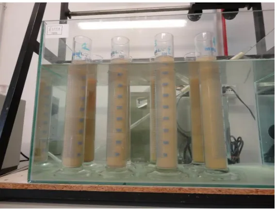
The analysis by the pipette method (Figure 5) followed the standard procedure as described by USDA-NRCS (2004), consisting in the following phases:

i) weighing 10 g of air dried soil sample <2mm;

ii) soil dispersion with 10 cm3 _{of a Calgon (0.2% vol) solution;}

iii) distilled water addition up to the final volume of 250 cm3_;

iv) agitating the suspension with horizontal agitator for at least 12 hours (150 rpm); cleaning the suspension at 250 m with distilled water;

v) topping up the passing fraction to the reference volume of 500 cm3 _{with distilled water;}

vi) analyzing the soil suspension volume (25 cm3_).

Figure 5. Soil particle-size analysis by the pipette method.

No pre-treatment for soil organic matter removal has been carried out on ReSolve project samples, since in this study the knowledge of the more "natural" particle-size distribution of the soil was of greater importance from a functional point of view. In that regard, Matthews (1991) assessed that the choice of including removal of organic matter, as well as that of carbonates and/or iron oxides, should correspond to the aim of the investigation and type of material to be analyzed.

The sedimentation analysis was carried out on a soil suspension passed through 250 µm sieve. The wet sieving procedure was employed to determine the sands larger than 250 µm; the wet sieving procedure was employed to determine the sands larger than 250 µm, but also the fine and very fine sand fractions, after that silt and clay analysis was completed.

Figure 6. Textural triangle for soil texture analysis using the USDA classification scheme (USDA-NRCS, 2004).

References

GEE G.W., BAUDER J.W. (1986). Particle-size analysis. In: Klute A. (ed.). Methods of soil analysis, Part 1, 2nd edn., ASA and SSSA, Madison, WI, pp. 383-411.

KETTLER T.A., DORAN J.W., GILBERT T.L. (2001). Simplified Method for Soil Particle-Size Determination to Accompany Soil-Quality Analyses. Publications from USDA-ARS / UNL Faculty. 305.

MATTHEWS M.D. (1991). The effect of pretreatment on size analysis. In: Syvitski, J.P.M. (Ed.), Principles, Methods and Applications of Particle Size Analysis. Cambridge University Press, Cambridge, MA, pp. 368.

USDA-NRCS (2004). United States Department of Agriculture - Natural Resources Conservation Service, Soil survey laboratory methods manual. Version No. 4.0. Soil Survey Investigations Report No. 42.

AGGREGATE STABILITY Materials needed

▪ 10.0, 4.75, 2.0, 1.0, 0.25, and 0.050 mm sieves ▪ Rubber hammer

▪ Vibrating sieve shaker

▪ Electronic-controlled sieving machine ▪ Numbered cans

▪ Digital balance with readability of 0.01 g ▪ Oven (105°C)

▪ Dispersing solution (containing 2 g ofsodium hexametaphosphate/L)

with a stroke of 4 cm per 10 minutes, at a rate of 30 complete oscillations per minute. The mass of oven-dried particles (105°C for 24 hours) in each sieve that resisted breakdown was determined. The mass of the fraction passing through the 0.050-mm sieve was thereby obtained by subtraction.

The respective dry masses were used to compute the MWD according to Van Bavel (1949), as follows:

MWD W i Xi

i n =

=



1

where:

MWD is the mean weight diameter (mm);

Xi is the arithmetic mean diameter of the i and i-1 sieve openings (mm);

W(i) is the proportion of the total sample mass (corrected for sand and gravel) occurring in the fraction (dimensionless);

n is the number of size fractions, including the one that passes through the finest sieve (in this case 6).

Figure 7. The electronic-controlled machine for aggregate stability analysis by wet sieving.

References

KEMPER W.D., ROSENAU R.C. (1986). Aggregate stability and size distribution. In: Klute, A. (Ed.), Methods of Soil Analysis, Part 1, Physical and mineralogical methods, 2nd Ed., Agron. Monogr. 9. ASA and SSSA, Madison, WI, pp. 425-442.

LEGOUT C., LEGUEDOIS S., LE BISSONNAIS Y. (2005). Aggregate breakdown dynamics under rainfall compared with aggregate stability measurements. Eur. J. Soil Sci. 56, 225-237.

VAN BAVEL C.H.M. (1949). Mean weight diameter of soil aggregates as a statistical index of aggregation. Soil Sci. Soc. Am. Pro. 14, 20–23.

PH AND ELECTRICAL CONDUCTIVITY (EC) Materials needed

▪ pH-meter

▪ Conductivity meter ▪ pH standard solutions

▪ Common laboratory equipment

fine earth are placed into a 100 ml wide-mouth type bottle with 100 ml water and shaken for 2 hours. The pH is measured by immersing a combination electrode in the upper part of the suspension.

For the EC measurement, it is recommended to let the soil:water mixture stand for another 2 hours after pH reading, then to filter it through a hardened low-speed filter paper. If the initial filtrate is turbid, it must be re-filtered using the same filter paper before EC measurement.

TOTAL CARBONATES Materials needed

▪ Calcimeter (Dietrich-Fruhling equipment or others) ▪ HCl

▪ Thermometer for room temperature measurement ▪ Barometer

▪ Common laboratory equipment

The total amount of carbonate in the soil is most commonly reported as total CaCO3 equivalent (the

analysis is not selective for calcite) and is usually measured by the gas-volumetric method. To this aim, different calcimetry equipments may be used (Dietrich-Fruhling, Scheibler, Bernard, De Astis, etc). Basically, soil samples are treated with a HCl solution; the evolved CO2 is measured manometrically and the amount

of CaCO3 equivalent is then calculated. According to the Dietrich-Fruhling calcimeter procedure, 0.5 to 5.0 g of the “fine earth” sample (depending on the presumed carbonate amount) is treated with 10 mL of 1:1 (v:v) HCl solution. The container used for treatment is manually shaken until complete CO2 development.

Room temperature and pressure must be recorded during the analysis to allow standardization at 0°C and 760 mm Hg of the CO2 volume developed. The final calculation takes into account the standardized CO2

volume (V0) and the sample weight (P), by the formula:

CaCO3 (g/kg) = (V0 x 0,0044655 x 1000)/P

Alternatively, the total CaCO3 equivalent may be determined by the “acid neutralization” method (sample

treatment by dilute HCl and titration of the residual acid).

TOTAL ORGANIC CARBON (TOC) AND TOTAL NITROGEN (TN) Materials needed

▪ Carbon/nitrogen elemental analyzer ▪ Tin-foil and Ag-foil capsules

▪ HCl

▪ Analytical balance (5 decimal points) ▪ Thermostatically controlled heating plate ▪ Common laboratory equipment

Soil samples without carbonates are directly analyzed for TOC and TN by weighing 40-60 mg of soil in tin capsules.

The instrument performance as well as calibration must be regularly checked, and a minimum of three aliquots for each sample (replicates) should be analyzed to check the consistency of results.

As an alternative to the dry-combustion technique, the Walkley Black and the Kjeldahl methods are suggested for TOC and TN analyses, respectively. Differently from dry-combustion, the organic C oxidation through the Walkley Black reaction is incomplete and an empirical correction factor of 1.3 is applied in the calculation of the result. Compared to dry-combustion, the Walkley‐Black and the Kjeldahl procedures are

more time‐consuming and requires extensive use of glassware. They, moreover, involves some health hazards and produces considerable amounts of polluting wastes.

CATION EXCHANGE CAPACITY (CEC) AND EXCHANGEABLE BASES (K, NA, MG, CA) Materials needed

▪ Ammonium acetate, 1 M, pH 7 solution

▪ Sodium acetate 0.9 M/sodium chloride 0.1 M, pH 7 solution ▪ Ethanol 96%

▪ Centrifuge tubes ▪ Mechanical shaker

▪ Whatman n. 42 filter paper

▪ Commercial standard solutions for AAS (K, Na, Mg, Ca) ▪ Atomic Absorption Spectrophotometer

▪ Commonly used laboratory equipment

The reference procedure for the analysis of CEC and exchangeable bases is the pH 7.0-buffered ammonium acetate (NH4OAc) method. Percolation in tubes may be replaced by shaking in centrifuge tubes. As

reference for detailed laboratory operations, the NaOAc pH 8.2 Centrifuge Method (5A2a) by USDA (Kellogg Soil Survey Laboratory Methods Manual, Version 5.0, issued 2014) may be used.

Summarizing, the sample is shaken 3-4 times in a centrifuge tube with a 1 M pH 7.0 NH4OAc solution (5 g

soil + 33 mL). The supernatants are collected together for the determination of the exchangeable bases. The sample is subsequently washed with ethanol and shaken 3-4 times with a pH 7.0 sodium acetate solution (33 mL). The excess salt is then removed with ethanol and the adsorbed Na is exchanged by repeated shakings with the pH 7.0 NH4OAc solution (33 mL). The supernatants are pooled together, and the

resulting solution is analysed by flame atomic absorption spectrophotometry (FAAS) for Na concentration, which is used for the calculation of soil CEC.

In order to quantify the exchangeable bases, the extract collected from the NH4OAc sample treatments is

made up to volume, filtered and subsequently diluted so that the analyte concentrations meet the calibration ranges (usually, 0-2.5-5-7.5-10 mg/L for both K and Na; 0-5-10-15-20-25 mg/L for Ca; 0-0.5-1.0-1.5-2.0- 2.5 mg/L for Mg). The concentrations of K, Na, Mg and Ca in the solutions are measured by FAAS, after calibration of the instrument. For spectrophotometer set-up and operation, it is recommended to refer to the manufacturer's manual.

Calibration standard solutions may be prepared either for a single element or for several elements (e.g., K+Na and Mg+Ca). They should have the same NH4OAc composition as the sample solutions.

Moreover, in order to overcome common interferences occurring in the flame, the addition of specific suppressors to both calibration and sample solutions is required (Caesium at a final concentration of 1 mg/mL for K and Na measurement; Lanthanum at a final concentration of 10 mg/mL for Ca and Mg measurement). The instrument readings for analyte concentration are in mg L-1_{. These are then converted}

to (cmol (+) kg-1_{) or mg kg}-1_.

Possible interpretations and conclusions

The pH 7.0 NH4OAc procedure often leads to overestimation of CEC in acid soils, especially for soils with

significant variable charges. Moreover, it easily introduces errors when applied to calcareous soils, due to the fact that high amounts of Ca are readily dissolved from carbonates at pH 7.0 and interfere with the CEC determination.

When CEC is not a diagnostic criterion for soil classification, e.g. saline and alkaline soils, the CEC may be determined at pH 8.2 (IUSS Working Group WRB, 2014).

Because of the dissolution of carbonates, the amount of Ca extracted from calcareous soils often greatly exceeds the exchangeable Ca. That’s why in calcareous soils the exchangeable Ca is routinely determined by the difference between the CEC and the sum of the other exchangeable bases (Mg+K+Na), and the base saturation is set to 100%.

Potassium and magnesium are two of the major nutrients for grapevine. Their exchangeable forms are in equilibrium with the soluble forms and contribute predominantly to the available pool for plants. For a correct interpretation of soil K and Mg values, they should be considered not only in absolute terms, but also in terms of the ratio of one to the other. In fact, an unbalanced Mg to K ratio could result in deficiencies in one element or the other, because of antagonism in the root absorption. On average, the

Mg/K ratio is considered to be “very low” when less than 0.5 (very likely induced Mg deficiency), “low” to “slightly low” between 0.5 to 2.0, “optimal” between 2.0 and 6.0, “slightly high” between 6 and 10, “high”

when higher than 10.0 (very likely induced K deficiency) (Fregoni, 2005; Sbaraglia and Lucci, 1994).

References

BURT R. (Ed.) (2004). Soil Survey Laboratory Methods Manual. Soil Survey Laboratory Investigations Report No. 42, USDA-NRCS, National Soil Survey Center, Lincoln.

FREGONI M. (2005). Viticoltura di qualità, Phytoline, Affi, Verona.

IUSS Working Group WRB, World Reference Base for Soil Resources (2014). International Soil Classification System for Naming Soils and Creating Legends for Soil Maps; World Soil Resources Reports No. 106; Food and Agriculture Organization (FAO): Rome, Italy.

SBARAGLIA M., LUCCI E. (1994). Guida all’interpretazione dell’analisi del terreno ed alla fertilizzazione. Studio Pedon,

Pomezia.

Part II: Monitoring of soil ecosystem service provision and

providers

Objectives

The level or intensity of soil services can be modified by soil management or restoration treatments. These changes are mainly associated with the quantity and the quality of organic matter in the first soil layers. Therefore, the analytical methods to monitor soil functionality in vineyards mainly focus on soil organic matter turnover and enzymatic activity. A list of selected service providers is proposed below, as indicators of high soil functionality and biodiversity.

Aims of ecosystem services and providers monitoring in soil are mainly to:

- Quantify the major soil functions linked to soil biota (soil organic matter turnover and nutrient recycling).

- Evaluate the abundance and the diversity of main soil service providers (earthworms, microarthropods or mesofauna, nematodes, fungi and bacteria).

Analyses to perform

Different techniques are available from literature:

Evaluated parameter Description of the assessment method

Organic matter breakdown using Tea-Bag Index Methodological sheet n°5

Earthworm monitoring Methodological sheet n°6

Enzymatic activity Methodological sheet n°7

Soil respiration Soil microbial biomass

Microbial communities through DNA extraction

Methodological sheet n°8

Soil mesofauna using Berlese extractors Methodological sheet n°9

Methodological sheet n°5: organic matter breakdown assessment using Tea-Bag

Index

Materials needed

For field work

▪ Lipton Green Tea Sencha ▪ Lipton Rooibos and Hibiscus Tea ▪ Shovel

▪ Marker pen ▪ Sticks

For laboratory work

▪ Drying stove (max 60°C) ▪ Scale with 0.001 g precision

How to proceed

The protocol is based on the methodology proposed in 2013 by Keuskamp et al. and available on

http://www.teatime4science.org/method/stepwise-protocol/. This technique consists of burying Lipton pyramid tea-bags for 3 months in the soil, twice per year (1-November to January, 2-April to June).Two types of teas are used, Green tea and Rooibos tea, the main difference being in their contrasting decomposability.

1. Measure the initial weight of the tea bag (.000 g).

2. Open a few bags and measure the bag weight without content (this is approx. 0.283 g) 3. Mark the tea bag codes on the white side of the label with a permanent black marker.

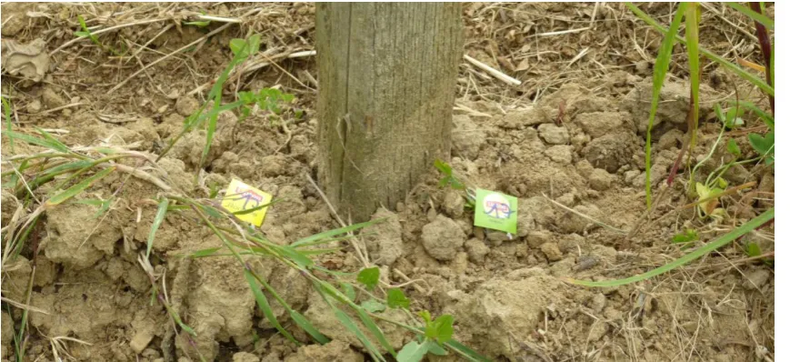
4. Bury the teabags in 8 cm-deep separate holes while keeping the labels visible above the soil (Figure 8), or otherwise tie the tea bags to a marked stick, to be able to find them back. Notice that tea bags could move in the soil due to soil erosion by water, therefore it is necessary to tie them to some hardly removable support.

5. Note the date of burial, geographical position, ecotype and experimental conditions of the site. 6. Recover the tea bags after approximately 90 days

7. Remove adhered soil particles, by gently tapping off the soil on the outside of the bags. Dry in a stove for 48h at 70 °C (not warmer!). Do not use water to remove the soil particles, because that invokes extra loss of material from the bag.

8. Remove what is left of the label but leave the string and weigh the bags (.000 g). Part of the label is paper and decomposes at a different rate as tea. Weight loss of the label may cause unwanted error in the measurement.

Possible interpretations and conclusions

The 2 types of tea show different values of carbon and nitrogen contents (Keuskamp et al. 2013) and decomposition dynamics. The C/N ratio is approximatively 12 for green tea whereas it is higher than 42 for rooibos tea. Rooibos tea decomposition is consequently slower and still in process after 90 days. Based on the weight of tea bags after exposure in the fields, we can calculate a TBI value, i.e., Tea Bag Index, which includes a degradation coefficient k and a stabilization factor S.

Moreover, the rate of decomposition of teas depends on soil parameters, mainly humidity, temperature, structure, compaction, and of course as a consequence, on soil biodiversity.

The comparison of k and S values allows to compare the quality and biological activity between different soils or to evaluate the effects of soil management practices.

Standardized Excel datafiles are available on http://www.teatime4science.org/data/submit-multiple-data-points/ to help with TBI calculation.

References

KEUSKAMP J.A., DINGEMANS B.J.J., LEHTINEN T., SARNEEL J.M., HEFTING M.M. (2013). Tea Bag Index: a novel approach to collect uniform decomposition data across ecosystems. Methods in Ecology and Evolution 4, 1070-1075.

Methodological sheet n°6: earthworms monitoring

Materials needed

For field work (sampling)

▪ Mustard (Amora® Fine et Forte) ▪ 40x40 cm frame

▪ Shovel ▪ Boxes ▪ Marker pen

For laboratory work

▪ Scale with g precision

When and where to sample

Earthworms should be monitored once per year in spring (April-May), at temperature between 6-15°C, no frost or drought, with presence of rainfall in the week prior to sampling and soil moisture around 10 to 25%.

How to proceed

To assess earthworm populations, mustard extraction method will be used (Lawrence and Bowers 2002): - Mix 90 g of hot mustard powder (Amora® Fine et Forte) with 100 ml of water in a closed bottle and

allowed to sit for at least 1 h. “Amora” can be replaced by other hot mustard powder, but the final allyl

isothiocyanate in the water solution should be about 0.025 g/l.

- Immediately prior to sampling, mix the mustard paste in a sprinkling can of 6 l of water.

- Place, at each sample site, a 40x40 cm metal, wooden or plastic frame on the ground and clear all the vegetation and leaves within it.

- Pour half of the mustard solution within the frame and a bit around, repeating the application a second time 10 min later.

- Take only the individuals emerging into the frame during 10 min after each mustard application. - Place the earthworms in an identified box.

- Dig the soil within the 40x40 cm to a depth of 25 cm and examine for the remaining earthworms. - Weigh the identified earthworms.

References

Methodological sheet n°7: enzymatic activities assessment

Materials needed

For field work (sampling) ▪ Shovel

▪ Plastic bags or boxes ▪ Marker pen

For laboratory work ▪ 2mm sieve ▪ Microplates ▪ Flasks

▪ Reagents (see method for details) ▪ Fluorometer

▪ Jar

▪ Ultraturrax homogenizer ▪ Manual pipettes

When, where and how to sample

Enzymatic analysis should be carried out once per year in spring time on soil sampled at two depths: 0-10 and 10-30 cm.

How to proceed

The samples should be air-dried (max 30°C), sieved at 2 mm and kept at room temperature until analyzed. Enzyme activity is measured according to the methods of Marx et al. (2001) and Vepsäläinen et al. (2001), based on the use of fluorogenic methylumbelliferyl (MUF)-substrates. Soil is analysed for N-acetyl-β -glucosaminidase (NAG), β-glucosidase (βG), butyrate esterase (BUT), acid phosphatase (AP), arylsulphatase (ARYL), β-xylosidase (XYL), cellulose (CELL) and acetate esterase (AC) activity using methylumbelliferyl (MUF) conjugated surrogate substrates (Sigma, St Louis, MO, USA). Briefly, 2 g of soil sample are weighed into a sterile jar and incubated for 24 hours at 20% soil moisture. A homogenous suspension is obtained by homogenizing samples with 50 mL deionized water with UltraTurrax at 9600 rev / min for 3 min. Aliquots of 50 µL are withdrawn and dispensed into a 96 well microplate (3 analytical replicates/sample/substrate). 50 µL of Na-acetate buffer pH 5.5 are added to each well. Finally, 100 µL of 1 mM substrate solution are added giving a final substrate concentration of 500 µM. Fluorescence (excitation 360 nm; emission 450 nm) is measured with an automated fluorimetric plate-reader (Fluoroskan Ascent) after 0, 30, 60, 120, and 180 min of incubation at 28 °C and enzyme activity will be expressed as nmol MUF g–1 _h–1_.

The order of magnitude of the values obtained for the different enzymatic responses varies considerably depending on the specific activity being determined, thus leading to some enzyme having more weight than others. To resolve this problem, the sum of the percentage of the maximum value found for a specific enzymatic response across all enzymes for a soil, was used for the calculation of the sum of enzymes (SUM). From this percentage of maximum enzyme activities, the Simpson-Yule index was calculated

following the equation E = 1/Σpi2, as indicated by Bending et al. (2004), where pi is calculated as a

proportion of enzymatic responses summed across all substrates for a soil.

Discriminant function analysis (DFA) is performed using soil enzymatic activities as grouping variables for soil and fractions. Squared Mahalanobis distances between group centroids are determined. Two significant discriminatory roots are derived and the results of DFA are graphically presented in two dimensions.

Possible interpretations and conclusions

the organic matter turnover and the availability of inorganic nutrients, providing indications on the function and quality of an ecosystem. The studied group of soil enzymes are hydrolases, which are involved in the main biogeochemical cycling of elements and release C compounds as well as N, P and S. Among hydrolytic

enzymes, β-glucosidase, α-glucosidase and β-cellobiohydrolase activities play a role in cellulose and starch degradation; phosphatases and arylsulfatase are involved in soil organic P and S mineralization; N-acetyl-β -glucosaminidase is involved in chitin degradation, a major source of mineralizable N in soil; N-acetyl-β -glucosaminidase and arylsulphatase activities are also considered as indirect indicators of the presence of fungal biomass because sulphate esters (substrates of arylsulphatase) are only present in fungal cells and chitin is the main constituent of fungal cell wall tissue. Hydrolytic enzymes have been frequently used as indicators of changes in quantity and quality of soil organic matter.

References

BADIANE N.N.Y., CHOTTE J.L., PATE E., MASSE D., ROULAND C. (2001). Use of soil enzyme activities to monitor soil quality in natural and improved fallows in semi-arid tropical regions. Applied Soil Ecology 18, 229-238.

BENDING G.D., TURNER M.K., RAYNS F., MARX M.C., WOOD M. (2004) Microbial and biochemical soil quality indicators and their potential for differentiating areas under contrasting agricultural management regimes. Soil Biol Biochem 36:1785–1792.

MARX M.C., WOOD M., JARVIS S.C. (2001). A microplate fluorometric assay for the study of enzyme diversity in soils. Soil Biology and Biochemistry 33, 1633–1640.

VEPSÄLÄINEN M., KUKKONEN S., VESTBERG M., SIRVIÖ H., NIEMI R.M. (2001). Application of soil enzymes activity test kit in a field experiment. Soil Biology and Biochemistry 33, 1665–1672.

Annex

• Table of substrates

Substrate Storage Quantity (mg) Solvent (µl) Buffer (ml)

MUF-cellobioside 4 °C 5.00 30 9.97

MUF-N-acetyl--D-glucosaminide - 18 °C 3.79 30 9.97

MUF--D-glucoside - 18 °C 3.38 30 9.97

MUF- phosphate - 18 °C 2.56 * 10.00

MUF-sulphate - 18 °C 2.94 30 9.97

MUF-−xyloside - 18 °C 3.08 30 9.97

MUF-butyrate - 18 °C 2.463 30 9.97

MUF-acetate - 18 °C 2.182 30 9.97

Methodological sheet n°8: assessment of soil respiration, microbial biomass and

communities

Materials needed

For field work (sampling) ▪ Shovel

▪ Plastic bags ▪ Marker pen

For laboratory work ▪ Beckers

▪ NaOH, HCl, K2SO4,ethanol-free CHCl3

▪ Thermo Flash 2000 CN soil analyser ▪ Mechanical shaker

▪ Whatman n. 42 filter paper

▪ DNeasy PowerLyzer™ PowerSoil® Kit

▪ Primers for V6-V8 region of bacterial 16S rDNA ▪ Gel electrophoresis material

▪ BIONUMERICS software

When, where and how to sample

Samples should be collected in spring (immediately before blooming) at two depths: 0-10 and 10-30 cm. 5 to 10 soil cores (depending also from the block dimension) for a total amount of approximately 2 kg should be collected, pooled together and then air dried and sieved at 2 mm.

How to proceed

Soil Respiration

At least 2 replicates per treatment (three plots per treatment) should be done. The method to be followed is described below.

Place 25 g of sieved soil sample in a 100 ml becker within a 1L stoppered glass jars together with 3 ml of 1M NaOH in a plastic glass. Incubate at 30°C and determine the CO2 evolved after 1, 3, 7, 10, 14, 21, 28 days

(replacing NaOH after each determination) by titration of the exceeding NaOH with 0.1 M HCl (Badalucco et al., 1992). The CO2 evolved during the 28th day of incubation will be used as the basal respiration value,

while the Basal Respiration Rate is measured as CO2 evolved in a defined time lapse.

Soil Microbial Biomass

At least 2 replicates per treatment (three plots per treatment) should be done. Microbial biomass carbon (MBC) and N (MBN) should be estimated following the Fumigation Extraction (FE) method (Vance et al., 1987): two portions of sieved soil (20 g each) should be incubated at 30°C for 24 hours in two different 50 ml becker; then the first one (not fumigated) should be immediately extracted with 80 ml of 0.5M K2SO4 by

oscillating shaking at 200 rpm for 60 min and filtering with Whatman paper n. 42; the second one should be fumigated for 24 h at 25 °C with ethanol-free CHCl3 in a vacuum dryer and then extracted as described

above. Organic C and N in the extracts should be determined by dry combustion on a Flash 2000 CN soil analyser (Thermo Scientific) and subtraction of non-fumigated values from fumigated ones.

Microbial communities through DNA extraction

Soil DNA direct extraction is performed on 250 mg of soil with DNeasy PowerLyzer™ PowerSoil® DNA

Isolation Kit (QIAGEN) by mean of FastPrep Instrument or MOBIO Power Lyzer or any equivalent soil bead beater instrument.

Subsequently DNA is amplified with primers specific for V6-V8 region of bacterial 16S rDNA in the condition outlined in Castaldini et al. 2005 and included below, and the mixture of three amplicons for each DNA are collected and run in a DGGE (Denaturing Gradient Gel Electrophoresis) gel as a single lane.

DGGE profiles are digitally processed with BIONUMERICS software version 4.6 (Applied Maths, St-Martens-Latem, Belgium): similarities between the banding patterns are analysed using Dice pairwise coefficients and hierarchical clustering of the Dice similarity matrix is determined using unweighted pair group method with arithmetic averages (UPGMA); finally a cluster diagrams is produced. The band profiles will be used in addition to count the number of bands to estimate richness of the most abundant bacterial populations in each sample and to calculate different biodiversity indexes (Shannon, Simpson; Pielou) (Boon et al., 2002; Lalande et al., 2013).

Possible interpretations and conclusions

Soil is a natural ecosystem whose energetic balance is determined by microbial biomass through respiration biogeochemical cycles. In agricultural ecosystems microorganisms play a key role in the transformation of nutritive elements and the maintenance of soil biological fertility. The Basal Respiration Rate is a measure of the microbial essential respiration involved in the total decomposition of organic matter, while the C extracted after fumigation may be used to estimate the soil microbial biomass. Finally, the metabolic quotient qCO2, that is the rate between basal respiration and microbial biomass C, can be calculated to

evaluate the ecosystem stability (Anderson, 1994): a low qCO2 value indicate a higher level of stability,

while a high level is generally associated with environmental stress.

The amplified DNA bands of each DGGE pattern give information about the bacterial diversity of a sample, as each band represent roughly a bacterial species, or more exactly, a bacterial phylotype or OTU (Operational Taxonomic Unit).

The UPGMA dendrogram of Dice pairwise similarity index of PCR-DGGE profiles illustrates separation of the profiles into clusters according to their percentage of similarity.

The number of bands estimate the species richness i.e the number of the most abundant bacterial populations in each sample.

The different diversity indexes evaluate the samples in terms of species diversity (Shannon Index that take in account the different bands and their relative abundance), presence of dominant species (Simpson Index), evenness of species (Pielou Index).

References

ANDERSON T.H. 1994. Physiological analysis of microbial communities in soil: applications and limitations. In Ritz K., Dighton J. & Giller K.E. (eds) Beyond the Biomass. John Wiley & Sons. Chichester (UK), pp. 67-76.

BADALUCCO L., GELSOMINO A., DELL’ORCO S., GREGO S., NANNIPIERI P. (1992). Biochemical characterization of soil organic compounds extracted by 0.5 m K2SO4 before and after chloroform fumigation. Soil Biology and Biochemistry,

24: 569-578.

BOON N., DE WINDT W., VERSTRAETE W., TOP E.M. (2002). Evaluation of nested PCR–DGGE (denaturing gradient gel electrophoresis) with group-specific 16S rRNA primers for the analysis of bacterial communities from different wastewater treatment plants. FEMS Microbiology Ecology 39: 101-112.

CASTALDINI M., TURRINI A., SBRANA C., BENEDETTI A., MARCHIONNI M., MOCALI S., FABIANI A., LANDI S., SANTOMASSWIMO F., PIETRANGELI B., NUTI M.P., MICLAUS N., GIOVANNETTI M. (2005). Impact of Bt Corn on Rhizospheric and Soil Eubacterial Communities and on Beneficial Mycorrhizal Symbiosis in Experimental Microcosms. Applied Environmental Microbiology, 71: 6719–29.

LALANDE J., VILLEMUR R., DECHÈNES L. (2013). A New Framework to Accurately Quantify Soil Bacterial Community Diversity from DGGE. Microb Ecol 66: 647–658.

Annex

• Protocol for DNA amplification

PCR Cycle Quantity referred to 25 µl reaction

Step Temp °C Time Cycles n. Reagents Starting Conc Q.ty µl

1 95 3' Primer GC968f 10 pmoli / µl 0,625

2 94 30" Primer 1401r 10 pmoli / µl 0,625

3 55 30" dNTPs 10 mM each 0,625

4 72 45" Buffer 5 X

5

5 Go to 2 34 MgCl2 25 mM 1,5 mM

6 72 5' DNA 5 ng / µl 2,5

7 4 forever Taq 5 U / µl 0,2

8 END Tot 11,075

H2O up to 25

• Conditions for DGGE run after DNA amplification

ACRYLAMIDE/BIS 40%37,5:1FINAL CONC IN GEL 6%

DENATURATION GRADIENT (7MUREA –40%FORMAMIDE) 50% - 60%

BUFFER TAE 1 X

RUN TEMPERATURE 60°C

VOLTAGE /AMPERAGE 75 V / 80 mA

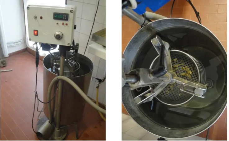
Methodological sheet n°9: soil mesofauna using Berlese-Tullgren extractors

Materials needed

For field work (sampling) ▪ Shovel

▪ Plastic bags or boxes ▪ Marker pen

For laboratory work

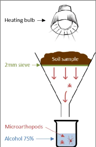
▪ Berlese-Tullgren extractors (funnel, heating lamp, 2 mm sieve, receptacle, alcohol 75%) ▪ Microscope

▪ Tubes or jars

When, where and how to sample

Sampling should be done to a depth of 10 cm, 1 dm3 _{(10x10x10cm) soil, in the middle of the row, avoiding}

the areas compacted by the tractor wheels. 3 sub-samples should be collected per treatment and homogenized in a single sample. Soil samples can be collected at different seasons, particularly Autumn and Spring, when arthropod abundances and diversity are higher.

How to proceed

The extraction of microarthropods should be carried out using Berlese-Tullgren extractors (Figure 9): - place a sieve (mesh of 2mm to allow the only passage of mesofauna) on the funnel.

- place above the funnel an incandescent lamp of 40 watts (about 20 cm from the sample).

- collect the mesofauna falling under the funnel in a preservative liquid consisting of alcohol 75° and Glycerine 5%.

Figure 9. A Berlese-Tullgren extractor

Soil microarthropod communities are studied according to the procedure described by Parisi et al. (2005), who defined the QBS index. Generally, the application of mesofauna-based indicators of soil quality have been limited by the difficulties in classifying organisms to the species level. To overcome this limitation, Parisi et al. (2005) introduced a new approach, based on the use of a simplified Eco-Morphological Index (EMI) for the determination of an QBS of arthropods index. This index is based on the concept that the higher soil quality, the higher will be the number of microarthropod groups adapted to the soil habitat. The degree of microarthropod adaptation is defined by specific morphological characters; in particular, more adapted organisms will typically show reduced pigmentation and visual apparatus, loss or reduction of wings, reduced appendages and streamlined body form (Parisi, 2001). Each biological form (morpho-type) isolated from the soil is classified to the order level and is eco-morphologically scored. The scoring is proportional to organism adaptation degree, ranging from 1 (surface-living organisms) to 20 (deep-living organisms). The sum of all EMI values for a given soil sample provides its QBS index.

Once determined, the QBS values can be used to define the QBS class, according to the classification given by Parisi et al. (2005). In particular, each class is identified by a number, ranging from 0 to 7, which increases with increasing complexity and adaptation degree of soil microarthropod communities.

Possible interpretations and conclusions

Berlese-Tullgren device combined with the use of morpho-types is a way to evaluate abondance and diversity of soil microarthropods while avoiding the complexity of taxonomy. Indeed, the use of indicators such as QBS index does not require a species-level identification. This index may be then considered as an appropriate tool for large-scale monitoring and based on a great number of samples. Soil microarthropods demonstrated to respond sensitively to management practices and be related to several beneficial soil functions and ecosystem services. It has for the moment to be developped and used in several systems and agrosystems in order to highlight its potential to characterize the effects of practices on biodiversity levels and associated services in soils.

References

PARISI V. (2001). The biological soil quality, a method based on microarthropods. Acta Naturalia de L’Ateneo

Parmense 37, 97-106 (in Italian).

PARISI V., MENTA C., GARDI C., JACOMINI C., MOZZANICA E. (2005). Microarthropod communities as a tool to assess soil quality and biodiversity: a new approach in Italy. Agriculture, Ecosystems and Environment 105, 323-333.

Methodological sheet n°10: nematodes monitoring

Materials needed

For field work (sampling) ▪ Hand auger ▪ Plastic bags ▪ Marker pen

For laboratory work

▪ Cotton-wood filter extractor ▪ Sieve 25 μm

▪ Stereomicroscope ▪ Microscope

When, where and how to sample

At each location, 5 cores (0 to 30 cm layer) should be randomly sampled and then mixed to form one composite sample of 500 cc of soil. Each soil sample should be placed in a plastic bag and stored at a 4°C cold chamber until use.

How to proceed

Free living and plant parasitic nematode should be isolated from 100 ml of each soil sample using the cotton-wood filter extraction methods (Oostenbrink, 1960). Nematodes are extracted for 48h at room temperature, approximately 25°C. Each nematode suspension is sieved through a 25 μm sieve and the

nematodes are counted at 50x magnification. Nematodes are mounted on temporary slides and identified at higher magnification to genus or family level using keys from Mai et al. (1964), Bongers (1988) and Marinari-Palmisano and Vinciguerra (2014). Taxonomic families are assigned to a trophic grouping based on Yeates et al. (1993).

The characterization of nematode communities should be done using:

(1) absolute abundance of individuals

(2) richness determined by counting the number of family

(3) Shannon-Wiener diversity index (H)

i s i i p p H ln 1



where pi represents the relative abundance of one given family;

(4) Simpson index (D)

(

)

(

1

)

1

−

−

=



N

N

n

n

D

where s is the number of species, N is the total number of organism, ni is the number of organisms of a

specie

(5) the Maturity (MI) and Plant Parasitic (PPI) indices by Bongers (1990), calculated as the sum of the weighted relative abundance of families classified in the cp scale for free-living and plant parasitic nematodes (c, colonizer nematodes r strategy; p, persister nematodes k strategy)

guilds responsive to physical disturbance in cp groups 3, 4, and 5. The CI is calculated as weighted ratio between fungal to bacterial feeding nematodes in cp groups 1 and 2 (Ferris et al., 2001). These indicators add information on functional guilds to develop food web.

Possible interpretations and conclusions

Shannon-Weiner and Simpson indices need a determination at species level to be representative. Generally, these indices underestimate their values because the specific identification is not always possible for nematodes.

Maturity and Plant Parasitic indices range from 1 (disturbed soil) to 4 (good soil quality) in a nematode community.

1 – indicator of organic pollution 2 – indicator of stress

3-4 – indicator of good soil quality

Food web indices: The combination between Enrichment index and Structure index highlights the soil conditions.

EI > 50 and SI < 50 values indicate high soil disturbance enrichment. EI > 50 and SI > 50 values indicate from low to moderate soil disturbance. EI < 50 and SI > 50 values indicate undisturbed soils.

EI < 50 and SI < 50 values indicate stressed soils.

References

BONGERS T. (1988). De Nematoden van Nederland. Utrecht: KNNV.

BONGERS T. (1990). The maturity index – an ecological measure of environmental disturbance based on nematode species composition. Oecologia, 83 : 14-19.

FERRIS H., BONGERS T., DE GOEDE R.G.M. (2001). A framework for soil food web diagnostics: extension of the nematode faunal analysis concept. Appl. Soil Ecol., 185: 13-29.

MAI WF, LYON H.H., KRUK T.H. (1964). Pictorial key to genera of plant parasitic nematodes. Ithaca (NY): Plates Reproduced by Art Craft of Ithaca Inc.

MARINARI-PALMISANO A. and VINCIGUERRA M.T. (2014). Classificazione dei nematodi. In : Ambrogioni L., d’Errico

F.P., Greco N., Marinari Palmisano A., Roversi P.F., editors. Nematologia Agraria generale e applicata, Società Italiana di Nematologia. Florence, 482 pp.

OOSTENBRINK M. (1960). Estimating nematode populations by some selected methods. In: Sasser J.N., Jenkins W.R., editors. Nematology. Chapel Hill: The University of Carolina Press, p. 85-102.

Part III: Soil rhizosphere monitoring

Objectives

Soil rhizosphere contains various micro-organisms. By monitoring them, it is possible to (1) assess microbial diversity in general, (2) isolate culturable microbes among them and (3) evaluate extent of colonization of roots by arbuscular mycorrhizal fungi. These parameters can then be compared and studied in relation with soil functionality status or soil restoration treatments.

Analyses to perform

Analyses on soil rhizosphere micro-organisms can target:

1. Microbial diversity in general, by using a culture independent approach. Principle of analyses:

- Obtain environmental DNA extracts from any microorganisms present in source sample (here rhizosphere soil or roots).

- PCR amplify phylogenetic marker loci with universal primers.

- Separate amplified products of DNA by exposing the mixture of amplicons to a gradient of denaturant in a polyacrylamide gel. Each electrophoretically separated band represents an individual bacterial / fungal species and band profiles represent bacterial / fungal communities. - Analyze the obtained number of bands per source sample to calculate diversity indexes.

- Analyze pattern of obtained band profiles for comparing communities of bacteria / fungi from different source samples, e.g. in Dice cluster analyses.

2. Culturable microbes, by isolating colony forming units from agar media. Principle of analyses: isolate rhizosphere soil or root associated bacteria / fungi by inoculating serial diluted source material on agar medium.

3. Extent of colonization of roots by arbuscular mycorrhizal fungi. Principle of analysis: directly visualize and quantitatively assess mycorrhization of roots by arbuscular mycorrhizal fungi.

Evaluated parameter Description of the assessment method

Assessment of communities and pure culture isolation of root- or rhizosphere-associated fungi and bacteria

- Assessing fungi and bacteria communities by generating fingerprints represented by PCR amplified phylogenetic marker genes

- Pure culture isolation of soil rhizosphere and root-associated bacteria and fungi

Methodological sheet n°11