Applications of Continuous Spatial
Models in Multiple Antenna
Signal Processing
Glenn Dickins
B.Sc.(ANU) B.Eng.(Hons) (ANU) M. Eng.(ANU) MBA (LaTrobe)
July 2007
ATHESIS SUBMITTED FOR THE DEGREE OFDOCTOR OFPHILOSOPHY OF THE AUSTRALIAN NATIONAL UNIVERSITY
Department of Information Engineering
Declaration
The contents of this thesis are the results of original research and have not been submitted for a higher degree to any other university or institution.
Much of the work in this thesis has been published or submitted for publication as journal papers or conference proceedings. These papers are:
• G. Dickins and L. W. Hanlen, “Fast calculation of singular values for MIMO wireless systems,” in Proceedings of the 5th Australian Communications Theory Workshop, (Newcastle, Australia), pp. 185–190, 2004.
• G. Dickins and L. W. Hanlen, “On finite dimensional approximation in MIMO,” in
Proceedings of the 11th Asia-Pacific Conference on Communications APCC2005,
(Perth, Australia), pp. 710–714, 2005.
• M. I. Y. Williams, G. Dickins, R. A. Kennedy and T. D. Abhayapala, “Spatial Limits on the Performance of Direction of Arrival Estimation”, in Proceedings of the 6th
Australian Communications Theory Workshop, (Brisbane, Australia), pp. 189–194,
2005.
• G. Dickins, M. I. Y. Williams and L. W. Hanlen, “On the dimensionality of spatial fields with restricted angle of arrival,” in Proceedings of the IEEE International
Sym-posium on Information Theory, (Adelaide, Australia), pp. 1033–1037, 2005.
• M. I. Y. Williams, G. Dickins, R. A. Kennedy, T. S. Pollock and T. D. Abhayapala, “A Novel Scheme for Spatial Extrapolation of Multipath,” in Proceedings of the 2005
Asia-Pacific Conference on Communications, (Perth, Australia), pp. 784–787, 2005.
• G. Dickins, T. Betlehem and L. W. Hanlen, “A Stochastic MIMO Model Utilising Spatial Dimensionality and Modes,” in Proceedings of the IEEE Vehicular Technology
• G. Dickins and R. A. Kennedy, “Angular Domain Representation of a Random Mul-tipath Field,” Submitted to EURASIP Journal on Wireless Communications and
Net-working, 2006.
• G. Dickins, M. I. Y. Williams and R. A. Kennedy, “Spatial limits to direction of arrival estimation,” Submitted to IEEE Signal Processing Letters, 2006.
The research represented in this thesis has been performed jointly with Professor Rodney A. Kennedy, Dr. Leif W. Hanlen, Dr. Terence Betlehem and M. I. Y. Williams. The substantial majority of this work is my own.
Glenn Dickins
Acknowledgments
During the time of my studies and research under the supervision of Professor Rodney Kennedy, I have been able explore a diverse range of theoretical and philosophical consider-ations related to spatial information theory. With a thirst for knowledge and understanding, I have been able to seek out and receive expert tuition whilst sharing many discussions and musings with experts in the field. I give thanks to all those who have gone before me and continue to clarify and distill the essence of research in this area. It is only now that I have moved into a different area of research that I fully realise the value and depth of the expertise I was exposed to in this field.
The pursuit of a PhD can be a long, arduous and largely solitary process, especially when it comes to writing the thesis. In my experience, there were two key factors which kept me going. The first was the time expended during the process of research and the desire to complete the degree. The second and by far the most important was the support, compassion, understanding, faith and gentle prodding of those around me towards submission.
First and foremost I would like to thank my wife Karen, without whom I would have been lost in despair more times than I care to admit. Karen, you are my one true companion through life and I thank you for always being there to help me maintain perspective and find the special moments in life. To my friends and family and parents who have stood by me through the highs and lows of the process, I thank you for being there and for believing in me. I am especially grateful for the time and encouragement given to me by Peter Fyfe, James Galloway and Jodi Steel. Thank you for providing the perspective to see beyond the doctoral process and not take it too seriously.
Lamahewa for their contributions and collaboration. I would also like to note and give thanks for the enjoyable time at the University of Uppsala and the chance to work with Professors Anders Ahl´en and Mikael Sternad.
Finally to my supervisors. I would like to give special thanks to Professor Rodney Kennedy for his wise and flexible supervision which fostered the exploration of far greater subject matter than is contained in this thesis. I would like to also thank Dr. Leif Hanlen for his supervision and contribution to the development of this thesis. I appreciate the assistance from my supervisors to help identify the key research results, develop the thesis structure and review the thesis content.
Abstract
This thesis covers the investigation and application of continuous spatial models for multiple antenna signal processing. The use of antenna arrays for advanced sensing and communi-cations systems has been facilitated by the rapid increase in the capabilities of digital signal processing systems. The wireless communications channel will vary across space as differ-ent signal paths from the same source combine and interfere. This creates a level of spatial diversity that can be exploited to improve the robustness and overall capacity of the wire-less channel. Conventional approaches to using spatial diversity have centered on smart, adaptive antennas and spatial beam forming. Recently, the more general theory of multiple input, multiple output (MIMO) systems has been developed to utilise the independent spatial communication modes offered in a scattering environment.
Contents
Declaration i
Acknowledgments iii
Abstract v
Contents vii
List of Figures xiii
List of Tables xvii
Notation, Symbols and Acronyms xix
1 Introduction 1
1.1 History and Background . . . 1
1.2 Multiple Antenna Communications . . . 4
1.2.1 Multiple Antenna Channel Framework . . . 4
1.2.2 Statistical Model of Channel Matrix . . . 6
1.2.3 Introducing Space into MIMO Channel Models . . . 7
1.2.4 Suggested MIMO Review Articles . . . 8
1.2.5 Review of MIMO Channel Models . . . 8
1.3 Motivation and Scope of Thesis . . . 10
1.4 Space, Waves and Intrinsic Limits . . . 12
1.4.1 Wave Equation . . . 13
1.4.3 Mutual Coupling . . . 15
1.4.4 Dimensionality . . . 16
1.4.5 Intrinsic Limits . . . 17
2 Dimensionality of Multipath Fields 19 2.1 Introduction . . . 19
2.2 Dimensionality of a Bandlimited Function . . . 22
2.3 Dimensionality of a Multipath Field . . . 24
2.3.1 Representation by Wave Equation Basis Functions . . . 25
2.3.2 Representation by Antenna Signal Subspace . . . 27
2.3.3 Comparison of Dimensionality Results . . . 28
2.4 Numerical Investigation of Dimensionality . . . 30
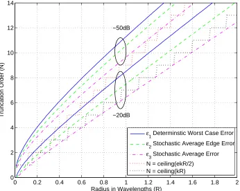
2.4.1 Bound for Worst Case Error Across Region . . . 30
2.4.2 Bound for Mean Error at Edge of Region . . . 30
2.4.3 Bound for Mean Error Across Region . . . 32
2.4.4 Discussion . . . 32
2.5 Development of Tighter Bound on Dimensionality . . . 34
2.5.1 New Upper Bound for the Bessel Function . . . 35
2.5.2 Application of New Bound to Dimensionality . . . 36
2.5.3 Discussion . . . 37
2.6 Impact of Near-Field Sources on Dimensionality . . . 38
2.7 Summary and Contributions . . . 41
3 Impact of Direction of Arrival on Dimensionality 43 3.1 Introduction . . . 43
3.2 Representation by Wave-Field Basis Functions . . . 44
3.3 Representation by Herglotz Angular Function . . . 44
3.4 Dimensionality of Multipath Field in a Region . . . 46
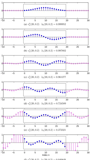
3.5 Slepian Series for Representing Bandlimited Sequence . . . 48
3.6 Dimensionality of Restricted Direction of Arrival Field . . . 51
3.7 Numerical Analysis of Multipath Dimensionality . . . 54
Contents
4 Angular Domain Representation of a Random Multipath Field 59
4.1 Introduction . . . 59
4.2 Problem Formulation . . . 61
4.2.1 Angular Domain Representation . . . 61
4.2.2 Random Multipath Field . . . 62
4.2.3 Finite Dimensional Representation . . . 64
4.3 Optimal Basis for Spatially Constrained Field . . . 65
4.3.1 Angular Representation of a Spatially Constrained Field . . . 66
4.3.2 Comments on Optimal Basis Representation . . . 72
4.3.3 Relationship to Karhunen-Lo´eve Expansion . . . 74
4.4 Angular Representation for Specific Configurations . . . 75
4.4.1 Circular Region with Isotropic Field . . . 75
4.4.2 Circular Region with Single Direction of Arrival . . . 77
4.4.3 Circular Region with Restricted Direction of Arrival . . . 78
4.4.4 Uniform Linear Array . . . 78
4.4.5 Other configurations . . . 79
4.5 Numerical Solution of the Eigenequation . . . 80
4.5.1 Nystr¨om Method . . . 80
4.5.2 Modified Nystr¨om Method . . . 81
4.5.3 Separable Kernel using Harmonic Exponentials . . . 83
4.5.4 Validation of Numerical Methods . . . 84
4.5.5 Discussion of Numerical Method . . . 88
4.6 Numerical Study of Angular Basis Functions . . . 89
4.6.1 Basis Functions with Non-Uniform Angular Power Spectrum . . . 89
4.6.2 Basis Functions for Elliptical Region . . . 89
4.7 Dimensionality of Optimal Representation . . . 90
5 Spatial Limits to Direction of Arrival Estimation 101
5.1 Introduction and Motivation . . . 101
5.2 Review of Direction of Arrival Literature . . . 103
5.2.1 Direction of Arrival Estimation . . . 103
5.2.2 Uncertainty in Direction of Arrival Estimates . . . 104
5.2.3 Number of Sources that can be Resolved . . . 105
5.2.4 Impact of Sensor Array Geometry . . . 105
5.2.5 Review and Discussion . . . 106
5.3 Numerical Investigation of Limits to DOA Estimation . . . 106
5.3.1 MUSIC Algorithm . . . 107
5.3.2 MUSIC Spectra for Multiple Sources . . . 108
5.4 Continuous Sensor Framework . . . 108
5.4.1 Continuous Field Model . . . 112
5.4.2 Noise Model . . . 112
5.4.3 Continuous Sensor Model . . . 114
5.4.4 Signal Model . . . 114
5.5 Bounds on the Performance of DOA Estimation . . . 115
5.5.1 Continuous Circular Array . . . 115
5.5.2 The Cram´er-Rao Lower Bound . . . 116
5.5.3 Cram´er-Rao Bound for Circular Array with Single Source . . . 117
5.5.4 Cram´er-Rao Bound for Circular Array with Two Sources . . . 118
5.5.5 Discussion of Two Source Result . . . 119
5.6 Numerical Analysis . . . 122
5.6.1 Analysis of Continuous Array Spatial Cram´er-Rao Bound . . . 122
5.6.2 Comparison with Discrete Sensor Cram´er-Rao Bound . . . 123
5.7 Comparison of Circle and Disc Array . . . 125
Contents
6 Stochastic MIMO Model Utilising Dimensionality and Modes 131
6.1 Introduction . . . 131
6.1.1 Background and Motivation . . . 131
6.1.2 Review of MIMO Channel Models . . . 133
6.2 New Framework using Continuous Spatial Model . . . 134
6.3 Discussion of the New Model Framework . . . 136
6.4 Simulation and Validation of New Model . . . 139
6.4.1 Approach for Model Comparison . . . 139
6.4.2 Description and Validation of Experimental Data . . . 141
6.4.3 Comparison of Performance of New Model . . . 144
6.4.4 Performance of New Model with Dense Antenna Arrays . . . 147
6.4.5 Use of New Model to Model Alternate Array Configuration . . . . 151
6.4.6 Use of New Model to Optimise Antenna Configuration . . . 152
6.5 Summary and Contributions . . . 155
7 Resolution of Spatial Location from within a Constrained Region 157 7.1 Introduction . . . 157
7.2 Problem Formulation . . . 159
7.3 Numerical Investigation of Distinct Localities . . . 160
7.3.1 Proposed Tiling Algorithm . . . 160
7.3.2 Numerical Examples of Location Tiling . . . 163
7.4 Intrinsic Limits of Resolving Spatial Location . . . 167
7.4.1 Localisation Horizon . . . 167
7.4.2 Number of Distinct Localities . . . 168
7.4.3 Application of Continuous Spatial Model . . . 171
7.4.4 Reflection in the Circle . . . 172
7.5 Localisation with Phase Coherent Receiver . . . 175
7.6 Discussion and Further Ideas . . . 178
8 Conclusions and Further Research 181
8.1 Overview of Contributions . . . 181
8.2 Open Problems and Further Research . . . 183
8.2.1 Relaxation of Narrow-band Assumption . . . 183
8.2.2 Impact of Using Suboptimal Spatial Basis Functions . . . 183
8.2.3 Parametric Spatial Basis Functions and Approximations . . . 185
8.2.4 Bessel Function Bound and Dimensionality . . . 185
8.2.5 Impact of Antenna Geometry . . . 186
8.2.6 Development of Consistent Noise Models . . . 188
8.2.7 Associated Spatial Dimensionality of a Single Antenna . . . 189
8.3 Closing Remarks . . . 191
A Interpolation of Dimensionality 193 B Derivation of the Cram´er-Rao Bound 197 B.1 Key Bessel Identities . . . 197
B.2 Derivation Overview . . . 198
B.3 Circular Array, One Source . . . 199
B.4 Circular Array, Two Sources . . . 200
B.5 Filled Disc Array, One Source . . . 203
B.6 Filled Disc Array, Two Sources . . . 204
Bibliography 207
List of Figures
1.1 Conceptual comparison of conventional and MIMO systems . . . 4
1.2 Compact form of MIMO matrix equation . . . 7
2.1 Numerical investigation of truncated field error . . . 33
2.2 New bound for leading edge of Bessel function . . . 37
2.3 Effect of near-field sources on dimensionality . . . 41
3.1 First six Slepian series basis forN = 20andW = 0.2 . . . 49
3.2 Dimensionality of field with restricted direction of arrival . . . 55
4.1 Schematic of region and angular spectrum used for validation . . . 85
4.2 Comparison of eigenfunctions for numerical methods . . . 86
4.3 Second comparison of eigenfunctions for numerical methods . . . 87
4.4 Eigenvalues and basis functions for uniform angular power spectrum . . . . 91
4.5 Eigenvalues and basis functions for field with Gaussian spectrum . . . 92
4.6 Eigenvalues and basis functions of field over elliptical region . . . 93
4.7 Essential dimension of field with restricted angular power spectrum . . . . 94
4.8 Essential dimension of field on elliptical region . . . 95
4.9 Effect of increasing angular spread on essential dimension . . . 96
4.10 Region geometries for analysis of offset in mean angle . . . 97
4.11 Effect of offset angle of arrival on essential dimension . . . 98
5.1 Simulation of direction of arrival estimation for multiple sources . . . 109
5.2 Effect of number of sensors on direction of arrival estimation . . . 110
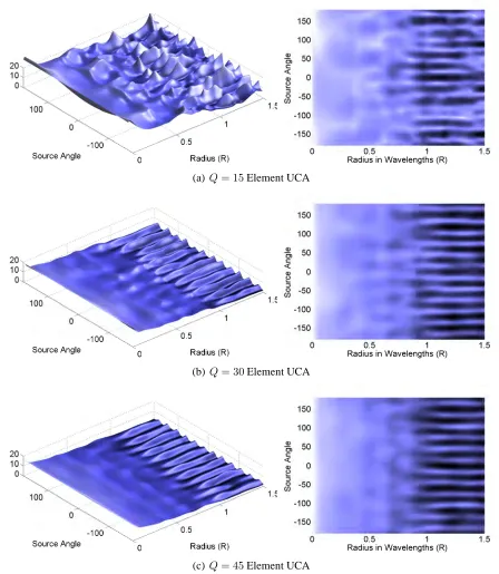
5.4 Relationship of SNR and source direction resolution for UCA . . . 120
5.5 Variance factor due to second source . . . 121
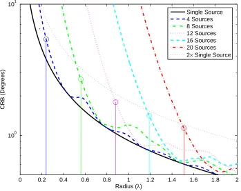
5.6 Effect of region size on Cram´er-Rao Bound for multiple sources . . . 124
5.7 Comparison of CRB for continuous sensor and 15 element UCA . . . 124
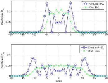
5.8 Comparison of coefficients for circular and disc arrays . . . 126
5.9 Comparison of Cram´er-Rao bound for a circular and disc array . . . 126
5.10 Comparison of circular and disc array variance factor . . . 128
6.1 Schematic of data path for models . . . 138
6.2 Validation of second order statistical model – mutual information and diversity142 6.3 Validation of second order statistical model – angular power spectrum . . . 143
6.4 Comparative performance of spatial model – mutual information and diversity 145 6.5 Comparative performance of spatial model – angular power spectrum . . . 146
6.6 Comparison or experimental and synthetic data . . . 148
6.7 Performance of spatial model for dense antenna array – MI and diversity . . 149
6.8 Performance of spatial model for dense antenna array – power spectrum . . 150
6.9 Sensor array geometries used for model prediction . . . 151
6.10 Prediction of performance of alternate array configuration . . . 153
6.11 Investigation of mobile station configuration using continuous spatial model 154 7.1 Schematic for set definitions in tiling algorithm . . . 161
7.2 Demonstration of tiling algorithm to determine resolvable locations . . . . 162
7.3 Location regions for 8 element uniform circular array . . . 163
7.4 Comparison of regions for 8 and 16 element uniform circular array . . . 164
7.5 Location regions for random sensor array geometry . . . 165
7.6 Location regions for different detection criteria . . . 166
7.7 Effective horizon for distinguishing source location . . . 169
7.8 Geometry for reflection of location regions in uniform circular array . . . . 173
7.9 Reflection of location space for uniform circular array . . . 174
7.10 Location with amplitude and phase . . . 176
List of Figures
8.1 Maximal point sets on the sphere of orderN = 50 . . . 187
List of Tables
4.1 Comparison of eigenvalues for numerical methods for spatial eigenequation 85
Notation, Symbols and Acronyms
Symbol Definition
ap source amplitude
a(θ) array response vector for directionθ
A A(θ) array response matrix
B2
R two-dimensional ball (disc) of radiusR
B3
R three-dimensional ball (sphere) of radiusR
Cm array response scaling constant for modem
ds(bθ) surface area element ofS2 D essential dimensionality
D(θ) derivative of array response matrix
e··· exponent function
E{· · · } expectation of a random process F space of far-field angular distributions
g(bθ) g(θ) angular domain representation function
gn(bθ) gn(θ) angular domain basis function
gN(θb) gN(θ) truncated finite dimensional angular domain representation
H MIMO channel matrix
HS modal channel matrix
Hn(·) Hankel function of ordern
I identity matrix
j =√−1 imaginary number
jn(·) spherical Bessel function of ordern
Jn(·) Bessel function of ordern
JR receiver modal configuration matrix JT transmitter modal configuration matrix
k = 2π/λ wave number
Symbol Definition
m mode or other integer index
M maximum mode or truncation order
MR mode truncation for receiver region
MT mode truncation for transmitter region
n time sample or other integer index
N number of time samples or max integer index
NR number of receive antennas
NT number of transmit antennas
p source number integer index
P number of sources
P(bθ) angular power spectrum
q sensor number integer index
Q number of sensors
r radius
R maximum radius of region
R covariance matrix
R real numbers
R2 two-dimensional space R3 three-dimensional space sinc(·) sinc function= sin(z)/z sp(n) source signal sample
s(n) vector of source signal samples
S minimum radius of sources
S1 unit sphere inR2, equivalent to[0,2π] S2 unit sphere inR3
S space of spatial fields
t continuous time
T maximum time
u(x) spatial field
u(x, n) spatial field at time samplen
U general functional space
wq(n) sensor noise sample
W modal coupling weight matrix
w(n) sensor noise vector
Notation, Symbols and Acronyms
Symbol Definition
y yq output signal
y y(n) vector of output signals
Yn Neumann function of order n
z arbitrary argument
zm(n) modal output signal
z(n) vector of modal output signals
αn coefficient of expansion
βn basis function
Γ(·) Gamma function
δ(·) Dirac delta function
δmn Kronecker delta function
ε error or small perturbation
σ2 noise variance
λ wavelength
λn eigenvalue
Λ spatial region of interest
Ω range of angular domainP(θb)6= 0 ρ(x,y) spatial correlation function
θ angle in[0,2π]
θx polar co-ordinate angle for pointx θp direction of sourcep
b
θ unit vector onS2
b
θx unit vector in direction of pointx φ angle in[0,2π]
b
φ unit vector onS2
△ Laplacian operator
k·kU norm of element in indicated space
| · | absolute value of argument
h·,·iU inner product of elements in indicated space [a, b] (a, b) closed / open interval fromatob
⊙ Schur-Hadamard elementwise matrix product ⊗ Kronecker matrix product
·T transpose of matrix or vector
·H Hermetian (conjugate) transpose of matrix ·−1 matrix inverse
−
Acronym Meaning
APS Angular Power Spectrum AWGN Additive White Gaussian Noise
BLAST Bell Labs Layered Space Time communications system CRB Cram´er-Rao Bound for variance of parameter estimation DOA Direction of Arrival
ESPRIT Estimation of Signal Parameters via Rotational Invariance Techniques MIMO Multiple-Input, Multiple-Output communications system
MMSE Minimum Mean Squared Error
MUSIC Multiple Signal Classification algorithm RMS Root Mean Squared average
SNR Signal to Noise Ratio UCA Uniform Circular Array ULA Uniform Linear Array
Chapter 1
Introduction
Any sufficiently advanced technology is indistinguishable from magic.
Arthur C. Clarke, 1961.
1.1
History and Background
For most of history, the ability of people to communicate without any physical connection was nothing but a magical fantasy. In 1865, James Clerk Maxwell published a seminal work showing that “an electromagnetic disturbance in the form of waves” could propagate through space [1]. This inspired work by Hertz, Marconi and Tesla that lead to the demonstration of wireless communication over significant distances at the dawn of the twentieth century. The concept of the mobile telephone emerged in 1947, with commercial systems becoming available in the early 1980s and rapid consumer uptake in the 1990s [2]. Now mobile phones are ubiquitous and an accepted part of our culture. The demand for wireless communica-tions continues to increase, driven by the high data rate connectivity requirements of mobile computing and multimedia devices.
A wireless device must be designed to meet the regulatory emission and bandwidth con-straints whilst also maximising battery life through low power usage. Such concon-straints moti-vate the search for ways to improve the efficiency of wireless communications systems – to send more with less. Understanding the wireless communications channel and how to fully and efficiently exploit it is an important area of research and development.
established the notion of capacity for a continuous communications channel in the presence of noise. For a channel with additive white Gaussian noise, the capacity is related to the logarithm of the signal to noise ratioη. For a channel of bandwidthB, the capacity is given by
C =Blog(1 +η) (1.1)
in bits per second using a logarithm of base 2. This represents an upper bound on the infor-mation that can be passed through the channel without error and is known as the “Shannon Limit”.
When multiple transmitters use the same frequency spectrum, the signal detected by a re-ceiver will be a combination of all the transmissions. For this reason, conventional sys-tems were developed with each independent broadcaster occupying a unique spectral band or spreading code1 within the range of radio coverage. Cellular systems were designed to achieve some level of spectral reuse over large distances. With this approach, the Shannon Limit implies that the only way to increase capacity is to increase the signal to noise ratio, or increase the signal bandwidth. The noise floor is not easily reduced and increasing the trans-mitted power results only in a logarithmic growth in capacity. Increasing the spectrum usage is generally not possible due to practical or regulatory constrains. For much of the twentieth century, this was thought to fundamentally limit the capacity of the wireless communication channel.
For mobile wireless communications, the variation of the channel characteristics over time and space presents many challenges [4]. There has been much research into ways of mitigat-ing or dealmitigat-ing with the effects of the fadmitigat-ing wireless channel. The variation of the wireless channel over space is known as spatial diversity Recently there has been a significant shift in the research community toward the idea of spatial diversity as an advantage rather than a problem for wireless communications. The basic principle centres around taking advan-tage of this spatial diversity in the communications channel by using multiple receiver and transmitter antennas.
Early work by Winters [5] hinted at the possibility of sending multiple streams of data si-multaneously using multiple antennas. Further research cemented the theoretical results [6] and practical architectures for achieving them [7]. Experiments at Bell Labs demonstrated these techniques in practice [8, 9], creating great excitement by effectively shattering the sin-gle channel Shannon Limit for communications spectral efficiency. The theory and practice
1Spread spectrum systems or code division multiple access systems utilise different spreading codes to
1.1 History and Background
suggested a capacity limit of the wireless channel that would increase linearly with the num-ber of antenna elements used. These events spawned the area of research and development known as MIMO (multiple input, multiple output) communications.
MIMO is now becoming accepted in practice with the recent IEEE standards 802.11n and 802.16e both providing for higher data rates using spatial multiplexing. Despite the exten-sive research and practical implementations of MIMO systems, there are some important questions that do not yet have satisfactory answers. The development of MIMO commu-nications theory, reviewed in the following section, stems from strong mathematical results for a general system with multiple inputs and outputs. Whilst the mathematical results are well established, there remains open questions regarding the applicability of such results to practical systems of multiple antennas. A critique of much of the research in this area is that the assumptions follow mathematical convenience rather than arising from a study of the physical MIMO communications system.
The underlying physical process responsible for wireless communications is the propagation of electromagnetic waves. A suitable model of this must be able to represent the associated physical value of the electric and magnetic fields continuously across a region of space. However, by construction, the central ideas in MIMO theory rest on the assumption that there is only a discrete set of input and output signals. The work of this thesis seeks to develop the ideas central to multiple antenna signal processing from the underlying perspective of a continuous spatial field. The development of the continuous spatial models to represent a wave-field is proposed as a way forward to improve the theoretical understanding and development of signal processing algorithms.
The use of a continuous spatial model permits the constraints inherent in electromagnetic radiation to be implicitly embodied in the signal processing frameworks developed. Research in this area will help to illuminate the physical processes and fundamental limitations critical to the performance of MIMO communications systems. The development of a continuous spatial framework will facilitate the effective representation, detection and signal processing for the physical electromagnetic fields that carry information. The goal is to extend the theory of MIMO communications systems beyond that of a discrete set of inputs and outputs, and to elegantly incorporate relevant aspects of spatial wave propagation.
(a) Conventional view of wireless communications. Space is filled by a broadcast as if it were a single dimensional pipe for information.
(b) MIMO wireless communications. Different spa-tial paths create spaspa-tial diversity at receiver and trans-mitter and allow re-use of the spectrum.
Figure 1.1: Conceptual comparison of conventional and MIMO systems. To the extent that each
received signal is a linearly independent combination of the transmitted signals, it is possible to exploit the channel as if it were multiple independent communications channels. Spectral reuse is facilitated by the spatial diversity of the transmitter and receiver antennas, along with the multiple propagation paths introduced by the scattering environment.
well developed frameworks, theorems and proofs. It provides a contribution to communica-tions theory to better reflect the medium over which the signal is being transmitted – in this case the spatial dimension.
1.2
Multiple Antenna Communications
The fundamental premise of multiple antenna (MIMO) systems is that the physical environ-ment in which the wireless signal is transmitted provides a degree of diversity through the existence of independent signal paths. With such spatial diversity, and through appropriate signal processing and detection, it is possible to achieve the transmission of multiple symbols using the same time and spectrum resource within a single wireless communications cell. To the extent that the received signal combinations are linearly independent, the channel can be utilised as if there were multiple independent channels. A conceptual comparison between the conventional view, and that adopted in MIMO systems, is shown in Figure 1.1.
1.2.1
Multiple Antenna Channel Framework
1.2 Multiple Antenna Communications
receiver antennas. We define s(t) = [s1(t)· · ·snT(t)]
T
as the vector of signals transmit-ted at time t. Assuming a linear system, the received signaly(t) = [y1(t)· · ·ynR(t)]
T is constructed by the convolution of the input signal with a set of channel impulse responses,
ym(t) = nT
X
n=1 Z ∞
−∞
hmn(t, τ)s(t−τ)dτ +wm(t) m = 1, . . . , nR (1.2)
y(t) =
Z ∞
−∞
H(t, τ)s(t−τ)dτ +w(t), (1.3)
whereHis a matrix of channel impulse responseshmn(t, τ)representing the contribution at timetof the signal at receive elementn from transmit elementmat timet−τ. The vector
w(t) = [w1(t)· · ·wnR(t)]
T
represents an additive noise process.
Depending on the signalling bandwidth, we need only consider samples of the baseband signals at an appropriate interval, T, such that y[n] = y(nT). The other signal vectors
s[n] = s(nT) and w[n] = w(nT) and sampled channel matrix H[n, k] = H(nT, kT). Assuming the channel is causal, we obtain a discrete time representation of the channel
y[n] = ∞
X
k=0
H[n, k]s[n−k] +w[n]. (1.4)
In the case of frequency flat fading, or where appropriate equalisation has been performed to eliminate inter-symbol interference, we can simplify the model to consider the transmission of a single symbol,
y=Hs+w, (1.5)
wheres is the transmitted symbol on the nT antenna, y is the received symbol on thenR antenna,His the instantaneousnR×nT channel transfer matrix andwis the noise vector. This equation represents the effect of each “channel use” and is the general signal framework adopted in works investigating the multiple antenna communication link such as [10]. For a given channel realisationHwe can calculate the theoretical channel capacity by con-sidering the number and strength of independent single dimensional channels supported by H. This is dependent on the rank and the eigenvalues ofHwith a value related to the loga-rithmic determinant of the system matrix [11]. The capacity will be
C =Blog det
InR +
η nT
HHH
(1.6)
bits per second for a base 2 logarithm, whereInR is the nR×nR identity matrix, and H
H
context of the components ofH having unity expected power. Provided there is sufficient transmitter diversity, the capacity can scale linearly with the number of antenna nR. This can be compared to the the single antenna case, (1.1), which would only allow a logarithmic increase in capacity as the addition of receiver antennas increased the effective signal to noise ratio.
1.2.2
Statistical Model of Channel Matrix
At typical radio frequencies, the presence of multiple signal paths and their subtle time varia-tions will cause random fluctuavaria-tions in the individual antenna coupling parameters ofH[4]. For such situations, it is expected that the value and statistics of the channel capacity will be of interest in a system design context.
Significant interest in the use of multiple antennas to achieve higher spectral efficiency in the wireless channel commenced around 1995. The mathematical results of Telatar and Foschini were key to demonstrating the potential for capacity gains when the channelHwas consid-ered as a statistical process [6, 12–14]. Some practical demonstrations soon followed that demonstrated such potential in laboratory environments [7–9]. These activities catalysed an explosion of research investigating the potential and realisable capacities for various classes of random matrixH. With a relatively simple channel model, (1.5), and armed with decades of statistical, matrix, and information theory many capacity results were presented as being informative of the practical MIMO communications problem [15].
Prior to the increased interest in MIMO, the statistics of a single antenna wireless channel were well studied. However, the statistics of the channel ensemble between two antenna arrays was a challenging and open problem. The application of a complete physical and electromagnetic propagation model had been considered for somewhat similar problems in optics [16] and introduced to communications [17]. In the case of a complex scattering environment such an approach becomes unwieldy and is best suited to specific geometrical investigations [18].
1.2 Multiple Antenna Communications
Figure 1.2: The compact form of the MIMO matrix equation. The discrete MIMO matrix equation
represents the effects of a broad range of complex physical properties and processes.
prompted work to introduce additional models for correlation between the channel com-ponents ofH[19–25]. There has also been significant interest in conducting measurement campaigns to fit empirical distributions to observed data [26–29]. Other efforts have sought to adopt convenient statistical distributions for analytic purposes [30–32]. A further review of MIMO channel models is presented in Section 1.2.5.
Such models provide a numerical framework to characterise antenna correlation, without ref-erence to the physical processes that cause it [25, 33–36]. Since these models are not directly related to the physical propagation, they can be misleading. For example, the framework per-mits degenerate “keyhole” channels [22, 37, 38], however in practice these are rare [39] and even difficult to reproduce in artificial situations [40]. The development of MIMO theory around statistical channel distributions became an independent research field, and arguably some results were of little practical significance.
1.2.3
Introducing Space into MIMO Channel Models
Around 2003, there was movement toward incorporating the spatial constraint of the MIMO arrays into the channel modelling. Some results suggested a finite dimensionality of a mul-tipath field over a region of space [41–43] and discuss the impact of this on channel mod-elling [44]. It was recognised that discrete statistical channel models ignored the fundamental aspects of wave propagation inherent in the problem [39, 45, 46].
The performance of a MIMO system will be directly related to the degree of spatial diversity available. However, for much of the MIMO literature, the spatial diversity and correlation of antenna channels was assumed or approximated. Ironically, to address this, the concept of “space” needed to be introduced in to the MIMO framework [47, 48].
specific to a particular antenna configuration, the use of a continuous spatial model moves closer to understanding the underlying dimensionality and appropriate representation of the spatial field.
1.2.4
Suggested MIMO Review Articles
Since the explosion in the level of research interest in MIMO systems, there has been numer-ous publications on the subject. This section presents briefly some of the more useful review and summary articles available.
One particular work [49] developed a wider interest in the field early on. A review by Gesbert et al. addresses theoretical and practical aspects of MIMO systems [50] with explanations and useful interpretations. Paulraj et al. present an overview of MIMO as the solution to meet the needs of high data rate links [51].
Special issues of the Journal of Wireless Communications and Mobile Computing [52, 53], EURASIP Journal on Applied Signal Processing [54], IEEE Transactions on Signal Process-ing [55] and IEEE Journal on Selected areas in Communications [56, 57] contain a collec-tion of relevant articles. Some key books on the subject have been compiled by Durgin [58], Jankiraman [59], Paulraj et al. [60], Gershman and Sidiropoulos [61] and Tsoulos [62].
1.2.5
Review of MIMO Channel Models
A fairly central theme of this work is the representation and modelling of the MIMO channel using the continuous spatial fields. Whilst there is some work in this area, the majority of MIMO channel models present a statistical model for the the discrete channel matrix specific to a given antenna configuration. This section presents a review of the literature in this area. The purpose of a channel model is to provide a way of capturing and simulating the behaviour of the channel matrixH. A good channel model should allow for the development and testing of systems to work in real practical situations. The quality and utility of a model depends on the intended application of the model and how well the model captures the parameters of the channel critical to the application [63]. A comprehensive review of the various MIMO channel models developed can be found in the work by Yu and Ottersen [64] and Jensen and Wallace [65].
1.2 Multiple Antenna Communications
with statistics based on experimental measurements or convenient probability distributions [22, 35, 36]. Given a system withnT transmitters andnRreceivers, characterising the corre-lations between the elements ofHrequires(nTnR)2parameters. Various models reduce this by assuming certain structures of the correlations. For example, the Kronecker model [23] assumes the overall correlation is separable as a product of receive side and transmitter side correlation. The virtual channel model [66] assumes a Fourier structure and the Weichsel-berger model [67] assumes a Kronecker style eigenbasis. Simple statistical models, such as the Kronecker, can provide satisfactory results for small numbers of antenna elements but will fail with more complex configurations [27, 68, 69]. Statistical models are easy to imple-ment and can provide adequate modelling for some purposes. The effects of the propagation channel and the transmit and receive arrays are coupled together in the resultant model. Geometrical or physical models characterise the spatial propagation aspects of the channel in terms of the directions of arrival and directions of departure [70]. Developed from early work on the nature of the time response of radio channels [71], the models incorporate the idea of distributed scatterers and clusters of scatterers interacting with the wireless signal. Models for the distribution and effect of scatterers can be based on geometric models, such as the one-ring and two-one-ring and other arrangements [72]. Alternately, the angular characteristics can be modelled as statistical processes [73]. Distributions such as the Laplacian [74] and Von-Mises [31] are used to characterise the angular spread of a scattering cluster. Such models can be fitted to experimental data by identifying scattering paths in array measurement data. This is typically achieved using subspace techniques for estimating direction of arrival. For specific physical scenarios, it is possible to use point wise ray tracing methods to model the channel [75]. With sufficient model detail, these have been shown to provide a good match to the physical measurements [76]. The experimental validation of channel models is an important area of research [29]. Complex models have been developed that incorporate many of the attributes discussed above and play a role in the development of future wireless standards [77].
1.3
Motivation and Scope of Thesis
There is an extensive amount of existing research on antennas and electromagnetic propaga-tion. The direct application of such results to the field of multiple antenna signal processing can create an onerous and often unnecessary level of complexity. The statistical models for MIMO analysis can provide an over simplification and be guided by mathematical ele-gance rather than practical correspondence. The motivation of this work is to develop the idea of continuous spatial model in a signal processing context in order to introduce a more appropriate level of complexity and physical correspondence to the MIMO problem. It is anticipated that this will be advantageous in the pursuit of understanding fundamental limits and achieving optimal system design.
In many practical applications, system design will be based on approximation or heuristics. While conventional designs may adopt a half wavelength antenna spacing, it is important to understand if this is efficient and optimal, or if there is room for improvement. Further-more, as the antenna array is extended in three-dimensional space, a single antenna cannot completely characterise the array geometry.
The motivation of this thesis is to understand spatial fields and multipath diversity to better inform system design, antenna geometries and signal processing used for multiple antenna communications systems.
Pioneering work in this area [41, 42, 44, 47, 78, 79, 82–84] has considered the limits of di-mensionality of a multipath field. The electromagnetic wave equation imposes a structure and constraint on the permissable wave-fields over a region of space. This work further de-velops the proposal of continuous spatial models to naturally incorporate this constraint into the problem formulation. The scope of the topics vary across optimal representations, pa-rameter estimation and statistical modelling in the area of multiple antenna systems. Since the work is largely exploratory, the contributions of the thesis vary in strength from reviews and observations through to detailed frameworks and theorems.
The structure and main ideas of the thesis are arranged as
follows:-• The remainder of this chapter provides some further background material related to electromagnetic fields and multiple antenna communications.
1.3 Motivation and Scope of Thesis
• Chapter 3 considers the specific problem of modelling a field with restricted direction of arrival. Formal proof of the relationship between dimensionality and angular spread is provided along with a constructive approximation for the optimal representation. • Chapter 4 contains a significant technical contribution of the thesis in the formal
devel-opment of the framework required to determine the optimal representation of a spatial field. It is shown clearly how the optimal basis depends on the angular power spectrum and the shape of the region of interest. Several examples are solved and investigated numerically.
• Chapter 5 presents a detailed derivation of a fundamental bound for system perfor-mance of direction of arrival estimation. This is a contribution in that the bound is independent of the specific sensor geometry and has been derived for multiple sources. It is shown that the number of sources that can be resolved is directly related to the essential dimensionality of the spatial field independent of the algorithm employed. • Chapter 6 presents a new continuous space statistical channel model. This model is
validated against experimental and simulated data and is shown to provide a more efficient representation of experimental data than existing models. By using the spatial model, this approach facilitates the prediction and optimisation of alternate antenna array geometries from measurement data.
• Chapter 7 presents an exploratory investigation of the implications of the continuous spatial model in the resolution of source location. Some new approaches are developed leading to some useful bounds for the problem defined.
• Chapter 8 offers concluding remarks and provides a set of open areas of research and conjectures that have been identified through this research work.
1.4
Space, Waves and Intrinsic Limits
Electromagnetic wireless communication requires the creation and detection of an electro-magnetic field. By controlling a current distribution across a region of space, the transmitter is able to generate or excite the field. The strength and direction of the electromagnetic field is a physical quantity that varies over space and time, extending beyond the region occupied by the transmitter. The continuous electromagnetic field, defined over the constrained re-gion of the receiver, carries information about the transmitted signal. The interaction of the electromagnetic field with antenna elements at the receiver will generate current and voltage signals.
Complete electromagnetic modelling of a MIMO system is generally prohibitive due to the scope of the propagation environment. A review by Jensen and Wallace [86] lists the physical parameters that are relevant to system performance:
• antenna sensitivity and impedance matching, • array size and configuration,
• element radiation patterns, • polarisation,
• mutual coupling, and • multipath propagation.
Modelling such parameters will increase the accuracy and applicability of the MIMO channel representation. This will provide a benefit when the increase in complexity is justified by a valuable improvement to matching and prediction of the model.
The first three of these items relate to the configuration of the sensor array. In practice, arrays should be designed to maximise their ability to transmit or receive information from the region of the electromagnetic field with which they interact. Jensen and Wallace suggest that the “average capacity is relatively insensitive to array configuration” [86], which leads to the concept of considering the intrinsic capacity of a region of space.
1.4 Space, Waves and Intrinsic Limits
1.4.1
Wave Equation
The physics and associated mathematics of wave propagation and wave motion is an area that has received a significant amount of attention [87, 88] and is accepted as a general en-gineering principle [89]. A similar theory can be applied across a wide range of physical waves, such as acoustic waves and electromagnetic radiation [90]. A central relationship is known as the reduced wave equation, or Helmholtz equation [91],
△u(x) +k2u(x) = 0, (1.7)
where u(x) is a scalar valued field representing some spatial property of the medium,
k = 2π/λ is the wave-number related to the wavelength, λ, of waves in that medium and△is the Laplacian operator equal to the sum of second order partial derivatives ofu(x)
on a unitary orthogonal co-ordinate system. For three-dimensional cartesian coordinates
△= ∂
2
∂x2 +
∂2
∂y2 +
∂2
∂z2. (1.8)
The second order differential equation (1.7) characterises the spatial distribution of a narrow-band wave-field across a region free of any sources. The time varying physical parameter is obtained from considering
U(x, t) = Reu(x)e−jωt (1.9)
whereRe{·}is the real component,j =√−1andω = 2πf is the angular frequency of the waves.
This equation is widely studied in acoustics where it is derived from a linearisation of Eu-lers’s equation and the equation of continuity for a compressible medium [91, 92]. The scalar field,u(x), is related to the velocity potential or localised pressure of the medium.
In considering electromagnetic radiation, we have the additional complexity of considering a vector field. The field at a point is fully characterised by six components – the electric field vectorE(x)and the magnetic field vector H(x). These fields must satisfy the vector Helmholtz equations,
△E(x) +k2E(x) = 0 △H(x) +k2H(x) = 0. (1.10)
complete constraint on the field can be expressed
△E(x) +k2E(x) = 0 ∇ ·E(x) = 0 H(x) = ∇ ×E(x)
ik or (1.11)
△H(x) +k2H(x) = 0 ∇ ·H(x) = 0 E(x) = −∇ ×H(x)
ik (1.12)
where∇is the vector differential operator
∇= ∂ ∂xi+
∂ ∂yj+
∂
∂zk (1.13)
for three-dimensional space with orthogonal unit vectorsi,jandkand respective cartesian coordinates(x, y, z). The divergence and curl operations on the vector field E(x)are then defined by the scalar or dot product and the cross product as∇ ·E(x)and∇ ×E(x). The divergence constraint implies that the electric or magnetic field has only two degrees of freedom. From this it is apparent that the complete electromagnetic field can be charac-terised by a two-dimensional scalar field satisfying the wave equation. A similar case for the importance of the wave equation was made in [93] where it was shown that the Green’s function for radiating waves satisfying Maxwell’s equations has two degrees of freedom. This brief analysis demonstrates why the properties of scalar fields satisfying the wave equa-tion (1.7) are central to understanding the limits of wireless communicaequa-tions. To facilitate the analysis, we will investigate the single dimensional scalar field. This approach matches physical implementations that make use of unpolarised antennas to interact with the field. The issue of polarisation will be discussed further in the next section.
1.4.2
Polarisation
Early work in the field demonstrated that different polarisation modes of the radio chan-nel could exhibit uncorrelated amplitudes [94]. The complete electromagnetic field has six components, suggesting that six communication modes are theoretically available [95, 96], however simple antenna designs will generally only excite or detect three modes [97]. Where the polarisation modes are independent, the use of polarisation will offer improved system performance in the form of a diversity gain [98].
1.4 Space, Waves and Intrinsic Limits
from one antenna location, the antenna itself must have some spatial extent to couple with the component modes of the electromagnetic field. It is likely that such results arising from the array may also affect the pattern or directional diversity [102].
In this work we consider scatterers to be a reasonable distance from the array and thus in the far-field. It is the far-field excitation and response of the transmitter and receiver array which are of interest. In addition to satisfying the wave equation, these response matrices will have two degrees of freedom. The use of polarisation could increase the available degrees of freedom by a factor of 2. In this way, limits of capacity or system performance utilising polarisation would be increased by a factor between 1 and 2 depending on the amount of cross polarisation diversity. This approach has also been followed by others to develop a MIMO spatial channel model incorporating polarisation [103].
1.4.3
Mutual Coupling
Practical antennas will exhibit coupling between the elements as they are brought close to-gether. This effect is known as mutual coupling. Initial studies of this effect [104–107] suggested a small improvement in system performance since mutual coupling would intro-duce antenna pattern diversity, decorrelating the antenna signals. Other works suggested the coupling would be detrimental [108] with a loss in signal to noise ratio degrading ca-pacity [109]. Practical measurements showed that degradation in radiation efficiency would outweigh any increase in pattern diversity leading to a loss in performance [110].
Whichever approach to mutual coupling is considered, the underlying field incident on the antenna array must satisfy the wave equation constraint. The mutual coupling effects and antenna impedance matching network can be considered to perform a processing operation on the wave-field. This can be well modelled by a linear transformation and consequently cannot increase the information content of the underlying spatial field [121]. Thus mutual coupling is a factor related to the efficiency of a particular antenna configuration, rather than having an impact on the fundamental limits for spatial communication.
1.4.4
Dimensionality
We define a continuous spatial field,u(x), to be a scalar function varying over three-dimensional space x = (x, y, z). We are interested in modelling the field over some domain of in-terest Λ ⊂ R3 which we require be bounded in extent such that x,y ∈ Λ implies that
kx−yk<∞. We also require thatΛis not a set of measure zero, and thus contains at least some open interval. We assume the field,u(x), is continuous, bounded and integrable over this domain. With these assumptions we can define an inner product and induced norm
hu, vi=
Z
Λ
u(x)v(x)dx kukΛ =
Z
Λ|
u(x)|2dx. (1.14)
DefineS as the space of fields u(x) created from this inner product and norm. The space S is isomorphic to a separable Hilbert space with countable basis. For example, a Fourier basis of spatial complex sinusoids can be easily constructed for an arbitrary region. Since the fields are continuous, the dimensionality of the space of fieldsSover the bounded region
Λwill be countably infinite.
If the fieldu(x)is required to satisfy the narrow-band wave equation, (1.7), this implies an additional second order differential constraint. DefineS′as the space of functions satisfying the wave equation (1.7) on the bounded regionΛ. The space S′ is a strict subspace of the spaceS and is again isomorphic to a countably infinite Hilbert space.
Consider a finite regionΛ′ ⊂Λwhose closure lies in the interior ofΛ. A similar norm can be
defined onΛ′ as in (1.14). Any member ofS′ with unit normkukΛ can be approximated on
the regionΛ′ with arbitrary precision with a fixed basisβ
m(x)form = 1, . . . , M for some
M <∞. That is, given an arbitraryǫ, there exists a numberM and set of basis functionsβm such that
min
αm
u−
M X
m=1
αmβm Λ′
1.4 Space, Waves and Intrinsic Limits
This result implies that provided a spatial field satisfies the wave equation over some larger regionΛ, an arbitrary field over a bounded finite volumeΛ′ ⊂ Λis essentially finite
dimen-sional. The combination of the wave equation constraint, a bounded domain of interest, and a finite precision representation leads to a fixed number of degrees of freedom. This is inves-tigated further in Chapter 2 and forms an underlying theme for this thesis. The notion that a field is essentially finite dimensional leads to results regarding the efficient representation of fields and fundamental limits to system performance.
The idea of dimensionality for the multipath spatial field in wireless communications was developed recently [41], leading to a string of results regarding capacity limits [82, 122– 124], modelling [44, 48, 78, 125], extrapolation [126, 127] and direction of arrival estimation [128, 129]. Similar ideas were developed by considering a suitable basis representation for the signals observed by a spherical antenna array [43, 84, 130].
The idea of dimensionality and degrees of freedom has been investigated for a scattered field resulting from objects in a finite volume [131–133]. This problem can be thought of as the dual of that considered in this work, where we are interested in the dimensionality of the electromagnetic field itself in a finite volume.
1.4.5
Intrinsic Limits
In wireless communications systems, transmission is achieved by means of a modulated narrow-band radio frequency transmission sent from a finite transmitter region and received in a finite receiver region. It follows then that the concept of the essential dimensionality of a wave-field developed in Section 1.4.4 will be related to the intrinsic ability to send infor-mation between the two regions. In the field of Wireless Communications and Inforinfor-mation Theory there have been several results presented towards understanding these limits. This section presents a brief literature review of that area.
The assumption of independently fading channel coefficients must be examined in the con-text of the wave equation [46]. The intrinsic limit can be related to the properties of a continuous operator describing the electromagnetic coupling between the two spatial re-gions [134, 135]. The laws of electromagnetism will have an effect on the maximum achiev-able spatial capacity [136, 137].
of a finite element approximation of the spatial channel [140]. The essentially finite dimen-sionality of the spatial field can be used to derive bounds for the scaling of the capacity of a constrained antenna array [79, 82]. An extensive numerical investigation has been presented with similar conclusions [121].
A recent detailed work by Jensen and Wallace reviewed the capacity saturation that results from considering the laws of electromagnetism [141]. A more mathematical approach based on the dimensionality of the spatial field is presented in [81].
Whilst this thesis will consider the application of continuous spatial models to several spe-cific problems, it does not extend to incorporate the capacity limits established above. The review in this section has presented the works that have taken the notion of the field dimen-sionality and applied it to the communications capacity problem. However, since some of the elements and aspects of the continuous spatial model remain poorly established, most of these results sit on tenuous foundations. The motivation of this research and thesis has been to provide a more systematic development of some of the aspects and applications of continuous spatial models.
Chapter 2
Dimensionality of Multipath Fields
2.1
Introduction
In engineering terms, the dimensionality of a system relates to the degrees of freedom or the number of intrinsic variables required to describe the state of a system. In practice, it is only possible to observe or control a system with a finite dimensionality. Provided such systems are also bounded in energy, they present a manageable level of complexity. We expect this to be the case for most physical systems over a bounded domain of interest.
When we lend mathematical models to physical quantities, it is possible to create a frame-work that permits unbounded dimensionality and complexity. For example, if we consider a simple continuous functiong(t)defined on the real intervalt∈[0, T], mathematically it can be bounded in both magnitude and energy and still exhibit a countably infinite complexity:
g(t) = ∞
X
n=−∞
αnej2πnt/T
∞
X
n=−∞
|αn| ≤1 ⇒ g(t)≤1
∞
X
n=−∞
|αn|2≤ 1 ⇒ Z T
0 |
g(t)|2 ≤T. (2.1)
capture information. The number of terms and their relative strength are directly related to the information theoretical limits of the system.
An understanding of the relationship between physical constraints and system dimensionality is an important problem. Consider the problem of a signal constrained to a duration of T
seconds and a spectral bandwidth ofWHz. The dimensionality of such a signal of2W T time is an accepted result that underpins much of communications and digital signal processing theory. Yet this result has a rich history and an extensive theoretical treatment with the key result presented by Slepian as the second Shannon Lecture in 1974 [85]
The approximate dimension of the set of bandlimited and time limited functions is asymptotically2W T asW orT becomes large.
For most applications, 2W T ≫ 1 and the asymptotic relationship is appropriate. Whilst the signal space is still infinite in dimensionality, any signal constrained in duration and bandwidth can be well approximated by a finite dimensional representation. The error in a representation decreases rapidly beyond the critical dimensionality. However, rather than this being an absolute threshold, it occurs across a span of the order oflog 2W T [142–145]. Thus for small 2W T the required accuracy can have a significant impact on the required number of dimensions.
The recent interest in using multiple antennas for communications has created an active area of research. Rather than considering a signal over a single dimension, we must consider a signal over three possible spatial dimensions in addition to time. Continuous functions are used to represent the variation of some physical property over the spatial region of the trans-mitter and receiver. In this work the physical properties considered are the electromagnetic field values. Therefore they have the additional constraint of Maxwell’s equations. We are interested in developing an understanding of the dimensionality or degrees of freedom in a continuous spatial field over a region of space. Such work will be fundamental to under-standing the limits and optimal approaches for transmitting and receiving information from within a confined spatial region.
2.1 Introduction
the idea of taking a volumetric approach to space has been developed [146] and the notion of an intrinsic capacity of the electromagnetic channel [136–139] has been presented. Whilst these publications are all relatively recent, the observation of a finite dimensional signal space based on the physical extent of the array, rather than the number of array el-ements, is not new. The practical approach has been to use antenna spacing no less than half a wavelength. Use of the Bessel expansion and principal terms for small ring arrays was established in the 1960s [147, 148]. The signals representing the principal components of variation across the antenna array were known as phase modes and have been applied to problems of direction of arrival estimation [149–153] and extrapolation [154]. The phase modes can be related to the signal from a virtual linear array [155]. The number of sig-nificant phase modes is related to the size of the circular array, not the number of antenna elements. Familiarity with the dimensionality of a spatial field in communications and infor-mation theory is still at an early stage. The attempts at creating a fundamental limit for the capacity of a region of space provide apparently conflicting and incomplete results.
This chapter presents an analytical and numerical study of the dimensionality and degrees of freedom of a continuous spatial field and its significance to the MIMO communications channel. It is a collection and extension of several works previously published by the author [156–158]. To provide some background, Section 2.2 reviews the framework for discussing the approximate finite dimensionality of a band-limited function. Section 2.3 extends this framework to consider a truncated representation of a two-dimensional multipath field. A discrepancy between the published results of Kennedy [41, 42] and Poon [43] is highlighted and explained. A numerical investigation of the truncation order and modelling error of a multipath field in Section 2.4 is used to demonstrate the applicability of the finite dimensional approximation and bounds. Section 2.5 presents new work to derive a tighter bound on the error and dimensionality of a multipath field, based on a new constructed bound for the Bessel function. As the bounds are developed under the assumption of far-field sources, Section 2.6 presents an analysis and investigation of the impact of near-field sources on the results.
2.2
Dimensionality of a Bandlimited Function
In this section we consider the degrees of freedom or dimensionality of a bandlimited signal with finite duration. It is true that no signal can be simultaneously limited in time and band-width. Thus we must consider signals which are effectively contained or almost limited, in some sense, to a given time and bandwidth. Without loss of generality, we assume a time signalg(t)with unity energy,
Z ∞
−∞|
g(t)|2 = 1. (2.2)
Adopting the approach set out by Slepian [85] we define a function as being “limited to a duration ofT at levelǫ” to imply that the fraction of the signal’s total energy outside of the interval[0, T]is bounded from above byǫ,
Z
t /∈[0,T]|
g(t)|2dt≤ε. (2.3)
Similarly, we can define a function as being “bandlimited to [-W,W] at level ǫ” with the bound
Z
|f|>W |
G(f)|2df ≤ ε (2.4)
where
G(f) =
Z ∞
−∞
e−2πjf tg(t)dt. (2.5)
Now considerGas the set of all unit energy functions time limited to[0, T]and bandlimited to(−W, W) both at levelε. Define the approximate dimensionalityN(W, T, ε, ε′)of G at
levelε′as the minimumN for which there exists a fixed collection of functionsΨ
1, . . . ,ΨN such that for anyg ∈ Gthere exists a set of coefficientsαnsuch that
Z
|t|≤T /2 g(t)−
N X
i=1
αnΨn(t) 2
dt≤ε′. (2.6)
The dimensionality theorem is stated as
lim
T→∞
N(W, T, ε, ε′)
T = 2W or Wlim→∞
N(W, T, ε, ε′)
2.2 Dimensionality of a Bandlimited Function
The works of Slepian, Pollak and Landau [142–145] derive the optimal set of basis functions
Ψnrelated to this problem. In these works they consider two classes of functions – those that are finite in duration with maximum concentration of spectral energy in a given interval, and those that are finite in bandwidth with a maximum concentration of energy in a given time interval. The case of signals concentrated in both a time and spectral interval was covered by Slepian in [85] and elegantly generalised by Franks [159]. These turn out to be a family of functions specified by the parameter2W T and scaled for the appropriate time and frequency intervals. The differential equation involved in this derivation is identical to that which arises in the separation of the wave equation in prolate spheroidal coordinates. As a result, these functions are known as the prolate spheroidal wave functions. It is the properties of these functions that are used to prove the dimensionality theorem.
A comprehensive formal framework representing over a decade of research was required to properly establish the dimensionality theorem for the one-dimensional time bandwidth case. Much of the work for this thesis is related to extending such results to the case of multi-dimensional spatial wave-fields. Despite the complexity underlying the formal results, it is evident that in the limiting case of a large dimensionality2W T, the exponential basis func-tions provide a reasonable approximation. This is consistent with the intuition and practical application of signal processing theory.
Taking the infinite basis expansion from (2.1) and definition (2.5)
G(f) =
Z ∞
−∞
e−2πjf tg(t)dt= ∞
X
n=−∞ αn
Z T
0
e2πjnt/Te−2πjf tdt (2.8)
=T e−jπf T ∞
X
n=−∞
(−1)nαnsinc (π(f T −n)) (2.9)
wheresinc(x) = sin(x)/x. From the maximum of 1 at f = n/T, |sinc (π(f T −n))|will decrease like|1/π(f T −n)|asn → ∞. Thus asT andW become larger, it is evident that the bound (2.4) is approximately satisfied provided that
αn≈0 ∀ |n|> W T (2.10)