Inter-Satellite laser interferometry

(1)

Inter-Satellite Laser Interferometry

Danielle Marie Rawles Wuchenich

A thesis submitted for the degree of Doctor of Philosophy

at the Australian National University

(2)

(3)

To my family and friends

here and afar

(4)

(5)

Declaration

This thesis is an account of research undertaken between February 2009 and February 2014 at the Centre for Gravitational Physics, Department of Quantum Science, in the Research School of Physics and Engineering at the Australian National University. This research was conducted under the supervision of Professor Daniel Shaddock and Professor David McClelland.

Except where acknowledged, the material presented in this thesis is, to the best of my knowledge, original and has not been submitted in whole or part for a degree in any university.

Danielle Marie Rawles Wuchenich February 2014

(6)

(7)

Acknowledgements

I cannot express enough gratitude to my supervisors, Professor Daniel Shaddock and Pro-fessor David McClelland, for their support and friendship over the years. Their guidance and generosity have created an atmosphere that has made for the most enjoyable place to work and learn. David—I have always admired your intelligence, kindness, and perspec-tive. I know I am not the first to point out that the exceptional dynamic of our group is a testament to how wonderful and wise of a leader you are—but I believe it wholeheartedly and it’s worth repeating. Daniel—you’ve become one of my best friends and mentors over the years. Thanks for teaching me everything I know and taking me on as your first student! To both of you—thank you for putting up with me all of these years, it is very bittersweet to be moving on as I’ve so thoroughly enjoyed my time here.

In each of my experiments, there were several people who made key contributions and I list them in the order in which the experiments are presented in this thesis (although chronologically it was nearly the opposite). The acquisition experiment was the most complicated experiment on which I have ever worked. I am so appreciative to Christoph Mahrdt, who came to ANU to work on the experiment with me, and for the fun we had both in and out of the lab. Several key contributions came from Ben Sheard, who graced us with his virtual presence on many occasions. The first acquisition experiment was set up by Sam Francis and Christoph with help from Conor Mow Lowry, and invaluable initial simulations were performed by John Miller. Throughout the saga, I had many insightful discussions with colleagues, notably Christoph, Ben, Robert Spero and Andrew Sutton.

The triple mirror assembly work was made possible by contributions from EOS, AEI, ACPO / CSIRO, and STI. I thank Conor for helping design and set up the test bed in Chapter 5. He also made the most useful lab gadgets ever, without which I would probably still be in the lab. I would also like to acknowledge and thank Roland Fleddermann, An-drew Sutton, and Captain Iain Elliot for various forms of support on this experiment. The work from Chapter 6 was performed with Roland Fleddermann and Robert Ward, with lots of generous support from Mark Blundell. These were some of my most entertaining lab days and I enjoyed working with you (and bossing you all around) very much. Rob and Roland—I think you can finally concede now that despite the spreadsheet you both were most certainly my postdocs. Set in (thesis) stone! I would also like to thank Craig Smith and the other folks at EOS and the AITC for watching out for us.

In my early fiber experiments, I received help from Timothy Lam on countless occa-sions, and have the most respect for his attitude, creativity, and more attitude. In addition I received support from Thanh Nguyen, Jong Chow, and Mal Gray—thank you all for be-ing generous with your time and advice. I would also like to thank Bram Slagmolen for taking time to share his knowledge and for always dropping everything to help anyone at anytime—you are a great asset to the group. Special appreciation to Andrew Sutton for years of friendship, technical babblings while sharing an office with me, and having to listen to my “phone voice.” Thanks also to James Dickson and all of the staff in the workshop for providing electronics and hardware for the experiments. The administrators, especially Kerrie Cook, made life as a PhD student so much easier. Much of the work in

(8)

this thesis was supported under the Australian Government’s Australian Space Research Programme.

The biggest thanks for the work in this thesis goes to Daniel Shaddock. I did not list his contributions or support under each experiment because he contributed to all of them, with unparalleled creativity and skill. Daniel—you are an exceptional scientist and I am so grateful to have had the privilege of working with you. You’re welcome for me teaching you all of my life skills, writing your research grants, and being “the girl” on your volleyball team so you could register in a mixed league.

I’ve had so many wonderful experiences throughout my program. I thank the JPLers for having me back to work every year, and am extra appreciative of Bill Klipstein for always making the effort to get me on lab no matter how short the notice! I never tire of being in the lab with the divine Glenn de Vine, THE Kirk McKenzie, Bob Spero, and Brent Ware—I truly have loved coming back every year and will always consider myself one of the gang. Who else would do the inter-lock tests?! I express my gratitude to Gerhard Heinzel and Karsten Danzmann for hosting me at AEI for three lovely months. The cohort of graviteers past and present that I’ve gotten to know continue to make work so enjoyable!! Notably Glenn, Daaf, Kirk, Dan, David, Sheon, Mal, Jong, Ian, Bram, Conor, Adam, Stefszky, Sutton, Tim, Thanh, Wade, John, Alberto, Rob, Roland, Dave, Silvie, Alison, Sam, Tarquin, Lyle, Georgia, Jarrod, Shasi, Ra, Phil, Richard (and honorary graviteers like Olli, Christoph, and Daniel). Sorry if I left someone out...! Extra thanks to the gravigals—Thanh, Silv, Georgia, Ali—for shoe talk and secret Max Brenner dates. No I love you more!

My career in physics began at Andrews, surrounded by wonderful friends and profes-sors, with special thanks to my adviser and physics mentor Margarita Mattingly. I am grateful to Guido Mueller and Bernard Whiting at the University of Florida for organizing the REU that introduced me to this field and first brought me to ANU. Thanks heaps to Emily, Alison, and my supervisors for aid and advice in writing and editing this thesis, and to Fritz for endless moral support.

(9)

Abstract

Subtle gravitational effects can be measured by precisely monitoring the position of a test mass. Often this is done by measuring the displacement between two or more test ob-jects. The Gravity Recovery and Climate Experiment (GRACE) satellites do just this, by continuously tracking changes in their separation with micron-level sensitivity. These dis-placement measurements are used to infer the gravitational potential of the Earth, which has enabled scientists to monitor key aspects of our climate since their launch in 2002. It is planned that the GRACE Follow-On satellites will include a laser ranging instrument as a technology demonstrator to improve the displacement measurement. Before science operation commences and measurements can begin, the laser on each satellite needs to be precisely pointed towards the opposite satellite, and thus the satellites must undergo an initial acquisition scan after launch to establish the laser link.

This thesis is concerned with developing technology for the GRACE Follow-On laser ranging instrument and exploring interferometric techniques for future satellite missions. In the following chapters, we experimentally demonstrate an acquisition system with GRACE Follow-On-like parameters, requiring no additional hardware but relying on the photodetectors and signal processing equipment already required for science opera-tion. This strategy was developed with multiple collaborators over several years led by C. Mahrdt at the Albert Einstein Institute. To establish the laser link, five degrees of freedom must be optimized (pitch and yaw for each beam, and the frequency difference between the two lasers). Laser steering and frequency scanning patterns are combined with a fast Fourier transform-based peak detection algorithm run on each satellite to find the signal. We successfully demonstrate both stages (commissioning and reacquisition) of the proposed acquisition strategy.

One of the core components needed for the GRACE Follow-On laser ranging instrument is the triple mirror assembly (TMA), a modified corner cube that symmetrically routes the laser beam around existing hardware about the satellite’s center of mass. A prototype triple mirror assembly was designed and constructed by local and international collabora-tors, and we present optical tests demonstrating three of the performance requirements of the prototype. The path length stability of a beam traveling through the TMA was mea-sured in a test bed resembling the measurement configuration of the GRACE Follow-On interferometer. The parallelism between the incoming and outgoing beams to/from the TMA is measured to the arc second level. Additional measurements quantify changes in the parallelism as the TMA prototype is heated and cooled.

Finally, we give a brief overview of digitally-enhanced interferometry, a developing tech-nique for optical metrology which has significant advantages over a conventional hetero-dyne system and could be employed for future space missions. We present an experimental demonstration of the multiplexing capability of the technique, showing an improved dis-placement sensitivity between measurement points when information from several sensors is combined to suppress errors due to laser frequency noise. We discuss an option for the technique to be applied to future inter-satellite measurement architectures and examine possible simplifications to the optical bench layout.

(10)

(11)

Overview and thesis structure

Laser interferometry has become a preferred method for making measurements between objects, as the displacement between two test masses can be monitored to unprecedented levels using an interferometric readout. It is planned that laser interferometry will be used in future space missions for ranging between satellites. Two planned missions are the GRACE Follow-On (GFO) mission to monitor changes in Earth’s gravity, and the Laser Interferometer Space Antenna (LISA) to measure gravitational waves of cosmolog-ical origin. Although the scientific goals of these missions are different, the underlying measurement technology is remarkably similar.

This thesis focuses on the development and testing of interferometric techniques for inter-satellite measurements and the application of these techniques to characterize pro-totype hardware for the GRACE Follow-On laser ranging instrument.

1.1 Thesis structure

The structure of the thesis is as follows. Chapter 2 provides an introduction to laser interferometry for optical metrology, focusing specifically on the interferometer for GRACE Follow-On.

Chapters 3 and 4 describe a strategy for initially acquiring the inter-satellite laser link after the GRACE Follow-On satellites launch. In Chapter 3, we present simulations of expected signal strengths and a point design of the acquisition strategy. In Chapter 4, we present the results of our experiment showing the successful demonstration of the strategy in the laboratory with GRACE Follow-On-like parameters. The experimental setup is described, along with a detailed characterization of several of the GRACE Follow-On parameters that we aimed to match in the laboratory.

Chapters 5 and 6 present optical tests of a prototype retroreflector needed to route the laser beam around the GRACE Follow-On satellites. In Chapter 5, we highlight designs of the primary prototype developed, and measure the path length stability of a beam traveling through the prototype. This test bed was built in the GFO laser ranging instrument measurement configuration. In Chapter 6, we measure the parallelism (co-alignment) between the beams traveling into and out of the retroreflector. We present measurements of the static co-alignment, as well as the measured co-alignment changes as the retroreflector is heated and cooled.

In Chapter 7, we give a brief overview of digitally-enhanced interferometry, a develop-ing technique for optical metrology which has significant advantages over a conventional heterodyne system. We present an experimental demonstration of the multiplexing capa-bility of the technique. We discuss an option for the technique to be applied to a LISA-like

(14)

measurement architecture and examine possible simplifications of the interferometer lay-out.

In Chapter 8, we provide a summary of the thesis and discuss options for future work.

1.2 Publications

The following is a list of publications related to this thesis to which I have contributed. Additional publications on the work presented in this thesis are in progress.

Glenn de Vine, David S. Rabeling, Bram J. J. Slagmolen, Timothy T-Y. Lam, Sheon Chua, Danielle M. Wuchenich, David E. McClelland, and Daniel A. Shaddock, “Picometer level displacement metrology with digitally enhanced heterodyne interferometry,”Opt. Express 17, 828-837 (2009).

Danielle M. R. Wuchenich, Timothy T.-Y. Lam, Jong H. Chow, David E. McClelland, and Daniel A. Shaddock, “Laser frequency noise immunity in multiplexed displacement sensing,” Opt. Lett. 36, 672-674 (2011).

David J. Bowman, Malcolm J. King, Andrew J. Sutton, Danielle M. Wuchenich, Robert L. Ward, Emmanuel A. Malikides, David E. McClelland, and Daniel A. Shad-dock, “Internally sensed optical phased array,”Opt. Lett. 38, 1137-1139 (2013).

R. L. Ward, R. Fleddermann, S. Francis, C. Mow-Lowry, D. Wuchenich, M. Elliot, F. Gilles, M. Herding, K. Nicklaus, J. Brown, J. Burke, S. Dligatch, D. Farrant, K. Green, J. Seckold, M. Blundell, R. Brister, C. Smith, K. Danzmann, G. Heinzel, D. Sch¨utze, B. S. Sheard, W. Klipstein, D. E. McClelland and D. A. Shaddock, “The design and con-struction of a prototype lateral-transfer retro-reflector for inter-satellite laser ranging,” Class. Quantum Grav. 31, 095015 (2014).

(15)

Chapter 2

Laser interferometry for GRACE

Follow-On

There have been a variety of experiments past and present to measure gravity. Some are fundamental tests of physics, with examples ranging from measuring Newton’s constant of gravitation G [1–4] to testing predictions of general relativity, such as the equivalence principle (e.g. STEP [5]), frame dragging (e.g. Gravity Probe B [6]), or gravitational wave detection (e.g. LIGO [7], LISA [8]). Other experiments are geodesy missions which measure the static or temporal gravitational potential of massive bodies from space (e.g. LAGEOS [9], GOCE [10], GRACE [11], and GRAIL [12] satellites). The above experi-ments vary in measurement apparatus, some situated on the ground and some deployed on satellites, from torsion balances to laser interferometers to gravity gradiometers based on atom interferometry.

Currently, laser interferometry provides the best precision when ranging between widely separated objects [13]. As changes in the optical path length are measured with respect to the wavelength of the light used, interferometry is able to measure very small fluctuations in the distance between objects.

The most sensitive laser interferometers are operating within the ground-based gravi-tational wave detectors, which aim to test a prediction of general relativity by looking for effects of astronomical events which cause the curvature of space-time to change [7]. Here, laser interferometry is employed to measure the change in distance between two isolated test masses, and this distance will fluctuate in the presence of a gravitational wave. The wave’s effect on the measurement output is commonly discussed in units of strain, that is, the fractional length change ∆Lover the total distance between the test massesL, giving

h= ∆L

L . In general, increasing the total distance Lbetween the test masses improves the

gravitational wave detector’s sensitivity. Unfortunately this becomes hard to do on Earth, as the test masses in the largest of gravitational wave detectors are already separated by 4 km and the entire path between masses is enclosed in a tube under ultra-high vacuum. Making similar measurements in space removes some of the challenges encountered with having the instrument on the surface of the Earth, particularly at low frequencies. The primary goal of the Laser Interferometer Space Antenna (LISA) [8, 14] is to measure gravitational waves from astronomical sources producing sub-Hz frequency waves. As in LIGO, laser interferometry will be used on LISA to range between the test masses on the satellites, although now the distance L between the test masses will be dramatically increased from kilometer-scale to gigameter-scale. Even the change in the arm lengths are anticipated to be many thousands of kilometers.

This is a thesis on furthering techniques so that laser interferometry can be utilized for inter-satellite measurements. Although laser interferometry has been used for decades to

(16)

make high precision displacement measurements, a laser interferometer operating between two satellites has not yet been flown. The first mission to do this will be the geodetic GRACE Follow-On satellites, planned to launch in 2017, where the laser ranging instru-ment will serve as a technology demonstrator [15]. The goal of the laser instruinstru-ment is to improve the ranging measurement made by the microwave instrument of its predecessor GRACE by a factor of 25. Many of the technologies for the GRACE Follow-On laser ranging instrument are available thanks to the decades of development for the ambitious requirements of LISA [15, 16].

This doctoral program was originally focused on exploring metrology techniques for a LISA-like mission, and some of the early work from the program with application to LISA is included in Chapter 7. The scope of my work changed when ANU joined a consortium to develop technology for GRACE Follow-On, and the majority of the work presented in this thesis is focused on interferometry for the GRACE Follow-On laser ranging instrument.

In this chapter we provide an introduction to the GRACE and GRACE Follow-On missions, and explain the layout and measurement of the GRACE Folllow-On laser ranging instrument. We also introduce the challenges of initially acquiring the laser link.

2.1 The GRACE & GRACE Follow-On missions

The Gravity Recovery and Climate Experiment (GRACE) is a joint NASA and DLR mission which monitors key aspects of our climate [17]. The twin satellites comprising GRACE fly in a polar, low-Earth orbit and employ a microwave ranging system to con-tinuously track changes in their separation with micron-level sensitivity over timescales of 1-1000 seconds. The displacement measurements (along with GPS and accelerometer data) have been used to produce monthly models of Earth’s gravity field [18]. Scien-tists have used this data to track water movement, such as changes in sea levels [19] and continental ground water [20], and over the past decade have quantified climate change phenomena, such as the melting of polar ice [21–24]. Now in nearly their 12th year in orbit, the satellites have well surpassed their planned five-year lifetime and their systems are starting to fail.

A new mission for data continuity, GRACE Follow-On (GFO), is planned to launch in 2017. In addition to the microwave ranging hardware, it is planned the satellites will also include a laser ranging instrument (LRI) as a technology demonstrator [15]. The satellites will exchange laser beams and use heterodyne interferometry to infer the change in their separation in the same way that the microwave instrument does. The laser ranging instrument is based largely on technology developed for the gravitational wave detectors LIGO and LISA, and should improve upon the microwave displacement measurement1

by a factor of 25. Although laser interferometry can easily achieve this performance in the laboratory, the low-earth orbit of GFO produces an environment where the thermal and alignment stability are much worse than, for example, their LISA counterparts [25]. Furthermore, as the GRACE Follow-On LRI is only a technology demonstrator, many additional constraints are placed on its design—such as mass, power consumption, and the placement of the LRI components on the spacecraft.

(17)

[image:17.595.120.542.96.321.2]

§2.2 The GRACE Follow-On laser ranging instrument 5

Figure 2.1: Planned laser ranging instrument design for GRACE Follow-On. Image repro-duced from Sheard et al. [15], with kind permission from Springer Science and Business Media [26].

2.2 The GRACE Follow-On laser ranging instrument

A detailed conceptual design of the GFO laser ranging instrument, along with the instru-ment description, is provided in Reference [15]. A schematic of the interferometer layout is reproduced here, in Figure 2.1, and we briefly summarize the role of the main components on each satellite:

• Laser with _≈1µm wavelength, which can be frequency stabilized to the on-board reference cavity.

• Fast steering mirror (FSM)to control the laser beam pointing in pitch and yaw to maintain continuous pointing to the other satellite by optimizing the interferometric contrast, while compensating for any attitude jitter and orbit perturbations.

• Beam splitter to interfere the local beam with light received from the distant satellite.

• Imaging optics to image the interfered beams onto the QPD while mapping any tilt in both the local beam and in the received beam from the distant satellite to tilt at plane of the detector.

• Quadrant photodetector (QPD) to detect the interference between the two beams at the heterodyne frequency.

(18)

• Triple mirror assembly (TMA), which is a corner cube retroreflector to balance the beam path around the satellite’s center of mass and return the outgoing beam parallel to the incoming beam.

Each satellite will record the phase of the heterodyne beat note via a digitally-implemented phasemeter [27]. A brief introduction to heterodyne interferometry is given in §2.2.2. The inter-satellite displacement—the desired science measurement—can be re-covered from the average phase measurements on each detector. Note that there will be one phasemeter channel per quadrant. The phases of the quadrants contain alignment information between the local and distant beams, allowing the steering mirror point-ing to be corrected in closed-loop to keep the interferometers optimally aligned. This approach—differential wavefront sensing—is a standard alignment technique [28] devel-oped for ground-based gravitational wave detectors [29] and is modified for use in hetero-dyne systems such as LISA Pathfinder [30, 31].

One of the core components of the LRI is the triple mirror assembly (TMA), a modified retroreflector consisting of three mirrors. Proposed by W. Folkner from the Jet Propulsion Laboratory, the assembly will be used to route the beam around the microwave ranging hardware on each satellite. Ideally the laser beams would travel directly between the satel-lites’ centers of mass. However, this direct line of sight will be obstructed by microwave ranging hardware and the cold-gas fuel tanks. The proposed off-axis measurement scheme for the laser ranging instrument uses the triple mirror assembly on each satellite to return the outgoing beam parallel to the incoming beam but translated by 60 cm (the distance required to circumvent the fuel tank). Normally in an off-axis measurement, satellite ro-tation will couple into the inter-satellite displacement measurement. However, the TMA’s virtual vertex will be placed at the satellite’s center of mass. Satellite rotation will still result in path length changes, but these changes will be anti-symmetric about the center of mass; if one of the one-way measurements between satellites is lengthened (due to rota-tion), the other one-way path will shorten. Thus by having the TMA strategically placed within the satellite, the range measurement will be less susceptible to errors caused by rotation.

When light is received from the distant satellite, the alignment of the local laser is continually adjusted by changing the angle of its onboard fast steering mirror so that its beam is transmitted to the other satellite at the same angle from which the distant beam entered. This sets a stringent requirement on the alignment of the three mirrors of the TMA—the alignment must be good enough so that TMA does not change the alignment of the outgoing beam by more than about 10% of the beam’s divergence. That is, the TMA must not change the alignment of the outgoing beam with respect to the incoming beam by more than 10µrad. This ensures that the beam is correctly directed towards the distant satellite. TMA design and assembly challenges, along with tests of a prototype, are presented in Chapters 5 and 6.

2.2.1 Desired performance of the laser ranging instrument

The target of the LRI is to improve the inter-satellite measurement sensitivity to 50 nm/√Hz at 0.1 Hz with degraded performance at lower frequencies [25], shown in Figure 2.2. This noise budget goal is

˜

x(f)< 50nm√

(19)

§2.2 The GRACE Follow-On laser ranging instrument 7

10

−4

10

−3

10

−2

10

−1

10

−9

10

−8

10

−7

10

−6

10

−5

10

−4

Frequency [Hz]

Pa

th

le

ng

th

no

is

e[

m/

√

Hz

]

[image:19.595.128.546.101.334.2]

LRI design requirement

Figure 2.2: Desired one-way path length noise for the laser ranging instrument.

where the noise-shaping function (NSF) is

NSF(f) =

s

1 +

f

2 mHz

−2

×

s

1 +

f

10 mHz

−2

. (2.2)

One of the biggest sources of noise for laser interferometric measurements in space is laser frequency noise (fluctuations in the wavelength of the laser). As the displacement is inferred with respect to the laser’s wavelength, changes in the wavelength are indistin-guishable from position fluctuations of the satellites. Thus, the laser’s frequency on one of the GRACE Follow-On satellites will be stabilized to its on-board reference cavity [32, 33]; we will refer to this as the master laser. The laser frequency noise requirement is set at 30 Hz/√Hz _× NSF(f). This performance has been surpassed in several laboratory exper-iments [34]. Even with this highly-stabilized laser, frequency noise will remain a dominant instrument noise source, limiting the LRI sensitivity over much of the measurement band [25].

The interferometer will be operated in an active transponder configuration [35], where the slave laser (the laser on the other satellite) will be offset phase-locked to the incoming light from the master laser. Conceptually, the distant satellite acts like an amplifying mirror, where the phase of the received light is preserved and the signal is amplified and returned to the local satellite. The offset frequency is selected to reduce technical noise in the phase-locking and keep the beat note between 2-18 MHz (the bandwidth of the electronics), which varies due to the Doppler shift as the satellites’ relative velocities vary in their orbit. As each satellite will have a reference cavity, the master / slave roles can be switched if, for example, one of the reference cavities fails.

2.2.2 Heterodyne interferometry

(20)

lasers’ frequencies _|f1−f2|. We discuss these two fields in the context of GRACE

Follow-On, and refer to Figure 2.1. If we examine the signals on photodetector 1, for example, we refer to laser 1 as the local beam and laser 2 as thedistant beam. In contrast, if we examine signals on photodetector 2, now laser 2 is the local beam and laser 1 is the distant beam. This convention is common in other GRACE Follow-On interferometry papers and will be used throughout this thesis.

The power measured over the photodetector area on each detector is

P =Plo+Psig+ 2 p

ηPloPsig

| {z }

Amplitude

cos(2πfhett+φ

| {z }

Phase

), (2.3)

where η is the heterodyne efficiency. The heterodyne efficiency is related to the inter-ferometric contrast κ (also known as the visibility) by κ = √η, and represents how well the two interfering fields are matched [38, 39]. On GRACE Follow-On, the beam from the distant satellite will have nearly spherical wavefronts by the time it reaches the local detector; on the scale of the photodetector area, the wavefronts are approximately planar. Thus the distant beam has a flat-top profile, and the resulting heterodyne efficiency is computed when it is interfered with the Gaussian profile of the local beam. This is shown in Figure 3.9 of Chapter 3 for various misalignment angles.

Referring to Equation 2.3, the power measured at the photodetector changes sinu-soidally with time t, and the sinusoid’s phase is related to the beat note frequency and optical path length changes in each beam path. A change in the optical path of one wave-length changes the phase of the heterodyne beat note by one cycle. Current techniques can measure changes in the beat note’s phase to the µcycle level [27]. Thus for optical interferometry with wavelengthsλ∼1 µm, fluctuations in path lengths on the picometer scale (10−12 _{m) can be sensed (although for GRACE Follow-On this will not be the case}

due to the level of laser frequency noise coupling).

2.2.3 Laser link acquisition

After the satellites are first launched, the lasers on each satellite need to be precisely pointed (in both pitch & yaw) at each other and their frequencies brought to within 20 MHz. There will be an initial unknown offset between the interferometer axis and the on-board pointing estimate provided by the Attitude and Orbit Control System, estimated to be up to ±3 mrad on each satellite. In addition to this pointing uncertainty, the offset between the laser’s frequency on each satellite will be unknown and is estimated to be up to func =±1 GHz. Thus an acquisition sequence covering all 5 degrees of freedom must

be performed to initially establish the laser link.

(21)

§2.3 Chapter summary 9

2.3 Chapter summary

(22)

(23)

Chapter 3

Acquisition for the GRACE

Follow-On laser interferometer

After launch of the GRACE Follow-On satellites, there will be an unknown offset between the interferometer axis and the on-board pointing estimate provided by the Attitude and Orbit Control System. This means that after everything is switched on, the satellites do not know where to steer their beams so that they are pointing at each other. This offset is estimated to be up to±3 mrad on each satellite.

In addition to this beam pointing uncertainty, there will be an unknown offset between the laser’s frequency on each satellite, estimated to be up tofunc=±1 GHz, much larger

than the bandwidth of the detector electronics (a frequency difference of 1 part in 108_{, or}

∼20 MHz). Thus before science operation can begin, an acquisition sequence is required to initially establish the laser link while scanning over these 5 degrees of freedom (pitch & yaw of each beam, and laser frequency difference) over their respective uncertainty ranges. Acquisition is a challenging problem and extensive simulations have been performed for generic inter-satellite laser links [40, 41], as well as specifically for LISA [42, 43] and GRACE Follow-On [44–47]. The GFO strategy differs from these other acquisition schemes as it does not utilize dedicated hardware or acquisition sensors, instead relying on the photodetector and signal processing hardware already required for science operation.

In§3.1, we present our analysis and simulations predicting the signal strengths on each satellite, and their dependence on beam misalignment. In §3.2, we outline an acquisition strategy devised by Christoph Mahrdt at AEI in collaboration with ANU and JPL, and present the results of Mahrdt’s more detailed simulations, as this is the baseline strategy that we will implement in the laboratory in Chapter 4. In §3.3, we briefly examine the statistics of the signals and noise in the signal processing chain during acquisition.

3.1 Simulations for expected signal strengths

In order to design an experiment to test possible laser link acquisition strategies, MATLAB simulations were performed to predict the signal strengths expected on GFO and verify results found by J. Miller/D. Shaddock (ANU) [48] and C. Mahrdt/B. Sheard (AEI) [49]. A working simulation verified with collaborators was necessary to make a representative laboratory experiment. The parameters used in the simulations were based on values expected for GFO provided by B. Sheard in Reference [25], in addition to discussions with R. Spero [50] and C. Mahrdt [49], and are listed in Table 3.1.

(24)

Quantity Symbol Value

Laser wavelength λ 1064 nm

Laser power P0 13 mW

Laser waist radius ω0 2.5 mm

Heterodyne beat note frequency (nominal) fhet 12.4 MHz

Beamsplitter transmissivity Tbs 0.05

Beamsplitter reflectivity Rbs 0.95

Photodiode radius rpd 4 mm

Photodiode responsivity ρpd 0.7 A/W

Local beam propagation distance zlo 0 m

Distant beam propagation distance zsig 270 km

Table 3.1: Select parameters used in our acquisition simulations.

3.1.1 Gaussian beams

Typically, laser beams are mathematically represented as Gaussian beams and are de-scribed by their radius of curvature R(z) and spot size w(z). In our simulations, we assume the beam produced by the laser is in its fundamental mode, where the beam has spherical wavefronts (related to the radius of curvature R(z)), and the irradiance distri-bution in the transverse direction (perpendicular to the wave’s propagation axis) follows a Gaussian shape with cylindrical symmetry about the propagation axis [51]. This is a reasonable approximation for the output of a single mode fiber (as used in GRACE Follow-On). This fundamental mode is referred to as the TEM00 mode1, and its electric field can

be written as

˜

E(x, y, z) =

s

2P0

πω2 0

ω0

ω(z)

e

−(x2₊_y2₎

ω2₍_z₎

| {z }

Amplitude

e

ik(x2₊_y2₎

2R(z) _e−itan −1 z zR eikz

| {z }

Phase

, (3.1)

where the wave’s direction of propagation is along the z axis (referred to as the optical axis) and by definition:

k= 2π

λ wave number, (3.2)

zR =

πω2 0

λ Rayleigh range, (3.3)

R(z) =z

1 +z

2 R

z2

radius of curvature, (3.4)

ω(z) =ω0 s

1 + z

2

z2 R

spot size. (3.5)

Note we’ve omitted the time dependent term e−i2πνt _(where _ν _{is the wave’s oscillation}

frequency and sweeps the phase through one cycle everyλ/cseconds) and the polarization

1

(25)

§3.1 Simulations for expected signal strengths 13

of the electric field.

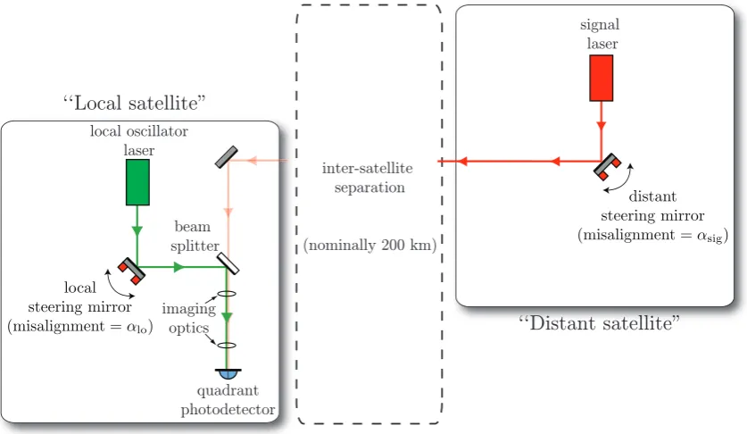
For the purpose of acquisition, the basic interferometric one-way ranging measurement can be thought of as that pictured in Figure 3.1. To find the resulting interference between

quadrant photodetector

signal laser

imaging optics

beam splitter ``Local satellite"

``Distant satellite" local oscillator

laser

inter-satellite separation

(nominally 200 km)

local steering mirror (misalignment =αlo)

[image:25.595.122.541.155.398.2]

distant steering mirror (misalignment =αsig)

Figure 3.1: Interferometric measurement concept on one satellite.

the two beams on the local satellite, the electric field of each beam is derived from Equation 3.1 and evaluated at the local satellite’s photodetector. Recall from §2.2.2 the resulting heterodyne beat note phase contains information about the spacecraft separation and the laser beam alignment. The on-board phasemeters will measure the phase of each quadrant, and the inter-satellite displacement measurement can be recovered by correctly combining the average phase on each detector.

These simulations aim to examine how the beat noteamplitude changes while varying the pointing of each beam αlo and αsig. This will enable us to determine the maximum

allowable misalignment in each beam after the acquisition sequence to give us a beat note amplitude strong enough that the phasemeter can reliably track.

3.1.2 ABCD matrices for ray tracing through an optical system

Equation 3.1 describes how the electric field of the beam evolves along the z axis. The amplitude of the field is highest along the optical axis, and drops off with a Gaussian shape in the transverse directions x & y. This can be combined with a ray optics approach to represent the field given various tilts of each beam due to changes in alignment of the steering mirrors. Given the planned waist size of 2.5 mm from Table 3.1, the beam divergence2_{(half-angle) will be}_θ

div = _πωλ₀ = 135µrad. A small divergence angle, where the

beam radius is large compared to the wavelength, allows use of the paraxial approximation [51]. This approximation—which applies as the beam makes small angles from the optical axis of the system under consideration and lies close to the axis3_{—enables system matrices}

to be used to describe the optical layout between the GRACE Follow-On satellites.

2

Assuming anM2value of 1. 3

(26)

An input ray with offsetyi and tilt αi,

yi

αi

, (3.6)

can be propagated through an arbitrary optical system to find the offset and tilt at the output. The resulting ray output can be described as

yo

αo

=

A B C D

yi

αi

, (3.7)

where theABCD matrix describes the properties of the system [51]. This system matrix approach was used to propagate the optical axes of the local and distant beams through our system, giving the offset and tilt of each optical axis with respect to a reference axis. The reference axis connects the center of each steering mirror to the center of the quadrant photodetector where the beam is to be evaluated. The ˜E field definition was applied to calculate the the electric field at these points around the reference axis. We assume each beam has a circular symmetry, where the spot sizes in each of the transverse axes are the same (ωx = ωy). We’ve also assumed that the beam-defining characteristics (waist,

wavelength, laser power) for each laser are the same.

Misalignments of the local and/or received beams — αlo and αsig — are included to

show how the detected beams are affected by various steering mirror angles. Note that each steering mirror can misalign in either pitchθ, yaw ψ, or both. The magnitude of the total misalignment α is

α=pθ2₊_ψ2_. _(3.8)

Imaging optics map beam tilt at the local steering mirror αlo or at the aperture of the

receive beam to pure tilt at the detector. The primary purpose of the imaging optics is to minimize the tilt-to-offset coupling. Otherwise, as the steering mirror is tilted to optimize interferometric contrast and steer the local beam toward the other satellite, the beam would walk off the detector area. This tilt-to-tilt mapping can be achieved using a lens system. B. Sheard shows mathematically this can be achieved using two lenses of focal lengths f1, f2 separated by a distance d2 [25], shown in Figure 3.2. Sheard shows

Object plane

d

1

d

2

d

3

f

1

f

2

Image plane

Figure 3.2: A two lens telescope, proposed for GRACE Follow-On, to achieve a tilt-to-tilt mapping from the steering mirror plane to the detector plane. Image from Reference [25].

that when lengthd2 is set such thatd2 =f1+f2 (the sum of the focal lengths), there is a

solution for the length d3 (between the second lens and the photodetector) such that the

matrix describing how the input beam responds to the lens system can be diagonalized according to

−f2/f1 0

0 ₋f1/f2

(27)

and tilt at the input maps into pure tilt at the output (and likewise for offset). This results whend3=−

f2

f1 2

d1+f2

1 +f2

f1

. This two lens telescope solution for tilt-to-tilt mapping was implemented in the laboratory setup, described in §4.1.4.

We do not directly include the imaging optics in this simulation, but instead apply their result. Beam tilts were performed in simulation by applying a coordinate transform via a rotation matrix, allowing the beam to be tilted with respect to the reference axis. As the waist of the local beam occurs at the steering mirror, it was imaged onto the detector by setting the detector position to zlo = 0 along the propagation axis; thus the detected

spot size equals the waist size (ω =ω0) and the radius of curvature is infinite (R =∞).

To capture 99% of the power in the local beam, the detector area was set so the radius

rpd>1.5ω0 [52]. The photodetector area may be smaller on GFO, but the imaging optics

will also result in a demagnification of the spot sizes, so our assumed ratio of the detector area to spot size is appropriate.

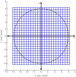
3.1.3 Numerical integration

The detection area was divided into a 300_×300 grid spanningrpd =±4 mm in thex&y

axes and the electric fields from both beams were evaluated at each grid segment. A 25×25 grid is shown in Figure 3.3 to convey the concept. Different masking functionsM(x, y) were

−5 −4 −3 −2 −1 0 1 2 3 4 5

−5

−4

−3

−2

−1 0 1 2 3 4 5

x axis [mm]

y

ax

is

[m

m

]

[image:27.595.205.459.381.638.2]

x y

Figure 3.3: Detection area divided into many grid segments for numeral integration. For illustrative purposes a 25×25 grid is shown here, however in our simulations a 300×300 grid was used.

(28)

large mask shown in Figure 3.4c, or by applying masks for the individual quadrants in Figure 3.4b and then summing the result. Both methods produced the same results in our simulations.

B

A

C

D

rpd g g (a)

B

A

C

D

rpd (b) rpd (c)

Figure 3.4: Different masking functionsM(x, y) applied in the simulations. (a) Quadrant detector of radius rpd with gap of width g. (b) Quadrant detector of radiusrpd with no

gap between quadrants. (c) Single element detector of radius rpd.

The electric field of the local beam on the local detector,Elo, is calculated by

numer-ically evaluating

Elo= s

2P0Tbs

πω2 0 e − x ω0 !2 e − y ω0 !2

eikψloxeikθloy (3.10)

at various steering mirror misalignmentsαloat the (x, y) coordinates in the detection grid.

The electric field of the distant beam (at the local detector), Esig, is found by

propa-gating its field over zsig= 270 km. When the beam from the distant satellite reaches the

local satellite, its wavefronts are nearly spherical4_{. However, on the scale over the detector}

area they are approximately planar, resulting in a flat-top profile. ThusEsig is calculated

according to

Esig= s

2P0R2_bs

πω2 0

ω0

ωsig(z)

e

− x−ψsigzsig

ωsig(z)

!2

e

− y−θsigzsig

ωsig(z)

!2

. (3.11)

Adding the electric fields of the local and distant beams at each grid segment gives the total field, both the DC (low frequency) and AC (high frequency) parts. The interfero-metric beat note – in the AC component – varies sinusoidally with time at the heterodyne frequency and is given by 2_<hEloEsig∗

i

. Depending on the relative tilt of the two beams, the phase of the interference at each grid segment could vary. Thus, to correctly deter-mine the beat note amplitude as measured by the detector, we perform the numerical integration of the complex interference over all grid segments

Z rpd −rpd

2EloEsig∗ M(x, y)dx dy (3.12)

for the various masking areas (each quadrant and the sum of the 4 quadrants). By first

in-4

(29)

tegrating over the complex interference term 2EloEsig∗ andthenevaluating the magnitude,

we solve for the amplitude directly and do not need to optimize the phase. 3.1.4 Beat note amplitude degradation with beam misalignment

These simulations predict how the beat note amplitude on each GRACE Follow-On satel-lite degrades as a function of steering mirror misalignment. For example, when tilting the local steering mirror in yaw only, e.g. αlo=θlo=±1 mrad, while the distant mirror stays

fixed, we get the response in Figure 3.5. Here, we have normalized for a total beat note amplitude of 1 for perfect alignment when detecting the sum of 4 quadrants.

−01 −0.8 −0.6 −0.4 −0.2 0 0.2 0.4 0.6 0.8 1

0.1 0.2 0.3 0.4 0.5 0.6 0.7 0.8 0.9 1

Misalignment in Yaw ψ [mrad]

N

or

m

al

iz

ed

b

ea

t

n

ot

e

am

p

lit

u

d

e

Sum of 4 quadrants

1 quadrant

Figure 3.5: Beat note amplitude degradation when misaligning the local beam in yaw, while the distant mirror stays fixed. The total amplitude is normalized to one for perfect alignment when detecting the sum of 4 quadrants.

Really we must examine how the beat note amplitude degrades with both local and distant misalignment, over the 3 mrad uncertainty expected for GRACE Follow-On. In general, the misalignments of the local and distant beams can be considered indepen-dently, as the local beam only affects the relative wavefront tilt whilst the distant beam misalignment predominately affects the received power at the local detector.

Local misalignment

Tilting the local steering mirror over αlo in any combination of pitch and yaw (while the

distant mirror stays fixed) yields the results in Figure 3.6. The response for the sum of 4 quadrants is shown in subfigures (a) and (b), and the response of a single quadrant is shown in (c) and (d). The left-hand plots show the responses in three dimensions, with their corresponding contours in the right-hand plots. Note that the area shown in these figures is only a small fraction of the total initial uncertainty.

(30)

−1 −0.5 0 0.5 1 −1 −0.5 0 0.5 1 0 0.2 0.4 0.6 0.8 1 Normalized beat note amplitude Local misalignment

in Yawψ[mrad]

Local misalignment

in Pitchθ[mrad]

(a) Sum of 4 quadrants.

Local misalignment in Yawψ[mrad]

Lo ca lm is a lignmen ti nP it ch θ [m ra d]

-1 -0.75 -0.5 -0.25 0 0.25 0.5 0.75 1 -1 -0.75 -0.5 -0.25 0 0.25 0.5 0.75 1 0.1 0.2 0.3 0.4 0.5 0.6 0.7 0.8 0.9

(b) Sum of 4 quadrants.

−1 −0.5 0 0.5 1 −1 −0.5 0 0.5 1 0.05 0.1 0.15 0.2 0.25 Normalized beat note amplitude Local misalignment

in Yawψ[mrad]

Local misalignment

in Pitchθ[mrad]

(c) Single quadrant.

Local misalignment in Yawψ[mrad]

-1 -0.75 -0.5 -0.25 0 0.25 0.5 0.75 11

-1 -0.75 -0.5 -0.25 0 0.25 0.5 0.75 11 0 0.05 0.1 0.15 0.2 0.25 L o ca l misalignme n t in Pit ch θ [mrad]

[image:30.595.55.485.101.492.2]

(d) Single quadrant.

Figure 3.6: Beat note amplitude degradation as a function of local beam misalignment, for the sum of 4 quadrants and a single quadrant. Three-dimensional plots are shown in (a) and (c), with corresponding contour plots in (b) and (d).

detector). This is because as the local beam misaligns, the relative tilt in wavefronts between the local and distant beams forms fringes across the detector. This effect was exploited in early acquisition strategies proposed by Miller and Shaddock [48]. Although the complex interference may add constructively over one quadrant, it can cancel when integrated over the entire detector area, resulting in a reduced beat note amplitude.

Although the beams are circularly symmetric, the individual quadrants are not, and so there is a dependence of the interference on the direction of misalignment when considering quadrants individually. For example, when misaligning the local beam along the 45o _axis,

note that in the single quadrant output the beat note degrades more quickly than for the same misalignment in pitch or yaw only.

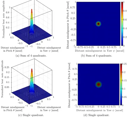
Distant misalignment

Misaligning the distant steering mirror byαsigin any combination of pitch and yaw (while

(31)

−1 −0.5

0 0.5 1 −1 −0.5 0 0.5 1 0.2 0.4 0.6 0.8 1 Normalized beat note amplitude Distant misalignment in Yawψ[mrad] Distant misalignment

in Pitchθ[mrad]

(a) Sum of 4 quadrants.

Distant misalignment in Yawψ [mrad] -1 -0.75 -0.5-0.25 0 0.25 0.5 0.75 1 -1 -0.75 -0.5 -0.25 0 0.25 0.5 0.75 1 0 0.2 0.4 0.6 0.8 1 Dista n t misalignme n t in Pit ch θ [mrad]

(b) Sum of 4 quadrants.

−1 −0.5

0 0.5 1 −1 −0.5 0 0.5 1 0.05 0.1 0.15 0.2 0.25 Normalized beat note amplitude Distant misalignment in Yawψ[mrad] Distant misalignment

in Pitch θ[mrad]

(c) Single quadrant.

Distant misalignment in Yawψ[mrad] -1 -0.75 -0.5-0.25 0 0.25 0.5 0.75 1 -1 -0.75 -0.5 -0.25 0 0.25 0.5 0.75 1 0 0.05 0.1 0.15 0.2 0.25 Dista n t misalignme n t in Pit ch θ [mrad]

[image:31.595.116.545.108.506.2]

(d) Single quadrant.

Figure 3.7: Beat note amplitude degradation as a function of distant beam misalignment.

the interference degradation is radially symmetric, even for the individual quadrants; less power is received at the local spacecraft independent of misalignment direction.

Remarks

In summary, as the local steering mirror misaligns, the beat note amplitude detected on both the local and distant satellites decreases. The beat note amplitude decreases on the local detector because of a relative tilt in wavefront between the local beam and the beam received from the other satellite, thus reducing the interferometric contrast. On the distant satellite, however, the beat note amplitude decreases because fewer photons reach the detector and contrast is unchanged.

(32)

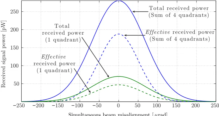
Effective received power

We calculated the total received power versus simultaneous steering mirror misalignment, where both steering mirrors were misaligned by the same amount (αlo = αsig) and the

result was evaluated. The results for the single quadrant and 4 quadrant sum are shown by the solid lines in Figure 3.8. Note that the total received power is independent of local beam misalignment. The effective received power—usable power that will contribute to a beat note—is found by multiplying the total received power by the heterodyne efficiency

η:

Psig, eff=ηPsig. (3.13)

The dashed lines in Figure 3.8 are the corresponding effective received powers at different

−250 −200 −150 −100 −50 0 50 100 150 200 250

50 100 150 200 250

R

ec

ei

v

ed

s

ig

n

al

p

ow

er

[p

W

]

Total received power (Sum of 4 quadrants)

Effective received power (Sum of 4 quadrants)

Simultaneous beam misalignment [µrad] Total

received power (1 quadrant)

Effective

[image:32.595.57.477.287.510.2]

received power (1 quadrant)

Figure 3.8: Total received power and effective received power as a function of simultaneous (local and distant) misalignment. The difference between the dashed and solid lines at zero misalignment is due to mode mismatch. The total received power is insensitive to local beam misalignment, whereas the effective received power is degraded by both distant and local misalignment.

steering mirror angles.

The phasemeter can reliably track 3 pW of effective received power per quadrant, so this sets the level of how precisely we must be pointed at the other satellite. Thus, we find the maximum misalignment that we can tolerate on each satellite that will yield the required power. From Figure 3.8, this corresponds to a simultaneous misalignment of 142µrad. Mahrdt refers to this as the worst-case misalignmentrwc needed for phasemeter

(33)

Comparison with Mahrdt’s results

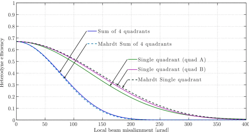
We compared our results with C. Mahrdt’s independent analysis at AEI [49]. In Figure 3.9 we show the comparison between our simulations of the heterodyne efficiency versus local misalignment. The results from the two simulations agree to within a few percent. The slight difference at larger misalignments could be due to the beams being approximated as Gaussian profiles in our simulations, whereas Mahrdt’s simulations more accurately modeled the output of a single mode fiber. Our calculations of the effective received power were also consistent—we both calculated a simultaneous misalignment of 142µrad corresponding to 3 pW of effective received power.

0 50 100 150 200 250 300 350 400

0 0.1 0.2 0.3 0.4 0.5 0.6 0.7 0.8 0.9 1

Heter

o

dyn

e

ffi

ciency

Sum of 4 quadrants

Mahrdt Sum of 4 quadrants

Single quadrant (quad A)

Single quadrant (quad B)

Mahrdt Single quadrant

[image:33.595.121.543.249.472.2]

Local beam misalignment [µrad]

Figure 3.9: Comparison of our heterodyne efficiency simulations with Mahrdt’s results showing consistency between our analyses.

Carrier to Noise Power Density Ratio

In reality, the phasemeter’s ability to track 3 pW of effective received power also depends on the level and distribution of noise present in the measurement. For this reason, specifying a carrier-to-noise-density ratioC/N0of a certain value is a more comprehensive requirement

to ensure reliable phasemeter tracking [53]. This number compares the signal power to the background white-noise power spectral density (the noise power in a 1 Hz bandwidth), and is often expressed in units of dB-Hz [54].

The resulting carrier-to-noise-density ratio given by 3 pW of effective received power is calculated below. The carrier power is determined by the strength of the beat note. The amplitude of the beat note incident on the detector is 2p

ηPloPsig (theseP values refer

to optical power). As the effective received power already incorporates interferometric heterodyne efficiency effects, we find the beat note amplitude according to 2p

PloPsig, eff.

To calculate the electrical power of the carrier, the beat note amplitude is propagated through photodetector’s electronics chain:

C[W_rms] = 2Psig, effPloρ

2 pdG2TIA

(34)

whereρpd is the detector’s responsivity in A/W,GTIA is the transimpedance gain in V/A,

and R is the resistance of the load in Ω. These detector terms will also be common to the noise chain so could be excluded from the analysis, as ultimately we will calculate the ratio between the carrier and noise contributions. We have also taken the 1/√2 factor into account when converting the 0-peak amplitude to an equivalent root-mean-square (rms) value, as we are calculating the power of the sinusoid [55].

For GRACE Follow-On, the noise at the heterodyne frequency is determined primarily by shot noise but also includes contributions from laser intensity noise and detector elec-tronic noise. Estimates of these single-sided spectral density noise levels were provided by R. Spero [50] and G. Heinzel [56] and are provided in Table 3.2. We calculate their noise

Quantity Symbol Value

Photodetector responsivity ρpd 0.7 A/W

LO power on 1 quadrant Plo 162µW

Effective signal power on 1 quadrant Psig, eff 3 pW

Shot noise on 1 quadrant N˜SN 8 pW/

√

Hz Laser relative intensity noise N˜RIN 3×10−8/

√

Hz Photodetector electronic noise N˜NEI 5 pA/

√

Hz

Table 3.2: Parameters and noise assumptions used to calculate the carrier-to-noise-density ratio C/N0 for GRACE Follow-On when each beam is simultaneously misaligned by

142µrad. The value of the laser relative intensity noise quoted here is at the lower fre-quency bin veto cutoff (_∼5 MHz).

powers so they can be directly compared.

• Shot noise: The incident power on the detector (for a weak signal beam, with strong local oscillator) gives a shot noise level of √2Plohν in W/

√

Hz [57, 58]. At the output of the detector this becomes (in noise density power)

N0, SN[W/Hz] =

2Plohνρ2_pdG2_TIA

R . (3.15)

• Relative intensity noise (RIN):The expected level of relative laser intensity noise ˜

NRIN at 5 MHz is shown in Table 3.2. The noise decreases at higher frequencies.

Below 5 MHz, the RIN dominates the noise, but these frequencies are ignored by rejecting them in a bin vetoing stage in the acquisition algorithm. For a given local oscillator power, the level of intensity noise becomesPlo·N˜RIN in W/

√

Hz. Converted to noise density power at the output of the detector this becomes

N0, RIN[W/Hz] =

P2

loN˜RIN2 ρ2pdG2TIA

R . (3.16)

• Photodetector electronic noise: The expected current noise generated within the detector (due to e.g. electronic shot noise and Johnson noise) is ˜NNEI. The

noise equivalent power can be deduced by dividing the noise equivalent current by the detector’s responsivity to give ˜NNEI/ρpd in W/

√

(35)

§3.2 Acquisition strategy 23

thus

N0, NEP[W/Hz] =

˜

N2

NEIG2TIA

R

= N˜

2 NEI

ρ2 pd

ρ2 pdG2TIA

R . (3.17)

The total noise power density is the sum of the contributing noise terms:

N0 = N0, SN+ N0, RIN+ N0, NEP. (3.18)

Thus, the resulting carrier-to-noise-density ratio is

C

N0

[Hz] = 2Psig, effPlo 2Plohν+P_lo2N˜_RIN2 +

˜ N2 NEI ρ2 pd . (3.19)

As C/N0 is often expressed in dB-Hz, Equation 3.19 becomes

C

N0

[dB-Hz] = 10 log₁₀



   

2Psig, effPlo

2Plohν+P_lo2N˜RIN2 +

˜ N2 NEI ρ2 pd      . (3.20)

With the numbers provided in Table 3.2, we calculate C/N0 = 68.6 dB-Hz. The GRACE

Follow-On project has set the requirement that the laser ranging instrument phasemeter is able to track beat notes with a minimum carrier-to-noise-density ratio of 67.5 dB-Hz per quadrant [50, 59]. Thus we will use this value (C/N0 = 67.5 dB-Hz) when setting the

experimental parameters in the laboratory.

3.2 Acquisition strategy

We can now predict how misalignments of the local and distant beam degrade the beat note amplitude and affect the ability of the phasemeter to track the interference. We must cover the 3 mrad uncertainty cone on each satellite with a spacing such that the maximum distance from any point to its nearest scan point (“nearest neighbor”) does not exceed

rwc = 142µrad. R. Spero refers to the distance between scan point centers as the grid

spacing, and is approximately 2rwc [60]. Recall in addition to the pointing uncertainty,

we have an unknown offset between the laser’s frequencies that could be well outside the bandwidth of our electronics. This means that even with perfect spatial alignment, if the lasers’ frequencies were offset by more than 20 MHz we would still not be able to measure the interference. Thus any acquisition strategy to establish the initial link for GRACE Follow-On must scan each of the 5 degrees of freedom over its respective uncertainty range. The goal is to bring the frequency offset between the lasers to within 20 MHz while aligning the two beams well enough such that the transition to differential wavefront sensing on each satellite can be established.

(36)

This approach was developed based on high fidelity simulations conducted over several years led by C. Mahrdt at the Albert Einstein Institute [44, 45] in collaboration with ANU and JPL. In this approach no additional hardware is required for the acquisition phase, instead relying on the photodetector and digital signal processing hardware used for science operation.

The acquisition strategy continues to be refined and the approach presented here rep-resents a point design and will likely be subject to further optimization. In this section we present the specifics of the strategy; the motivation and nuisances that went into choos-ing this method are found in Mahrdt’s thesis [45]. My major contribution to this work is the design and successful experimental demonstration of this approach, described in Chapter 4.

Our acquisition approach is broken into two parts: a commissioning scan and a reacqui-sition scan. The commissioning scan is a large-range scan envisaged to be performed once after launch, and will take significantly longer and may require input from the ground. The reacquisition scan is a smaller-range, faster scan that will be used after the initial uncertainties are known from the commissioning scan, and is designed to be autonomous.

Quadrant A Quadrant B Quadrant C

Quadrant D

+

Bin Veto Maximum

4096-point

FFT |Amplitude|

2 real

imag from

Figure 3.10: Signal processing on the FPGA during the commissioning and reacquisition scans.

A block diagram of the acquisition digital signal processing is shown in Figure 3.10. As mentioned, no new equipment will be added—the hardware already in place for science operation will be utilized, and the acquisition algorithms used for the commissioning and reacquisition scans will be implemented on the Laser Ranging Processor’s (LRP) field pro-grammable gate array (FPGA), which runs the phasemeter during science operation. Each photodetector quadrant is digitized by an analog-to-digital converter (ADC) and sent to the on-board FPGA for peak detection. Note that in science operation, each quadrant will have its own channel for phasemeter processing. In acquisition mode, however, each quad-rant will be digitized and immediately added with the signals from the other quadquad-rants to form the 4 quadrant sum on the FPGA mimicking a single element detector. A 4096-point FFT is continuously performed on this summed channel on each satellite during the spatial and frequency scanning. The resulting real and imaginary parts are combined to yield the signal power in each bin (this is described in more detail in §3.3). After every FFT, the bin with the highest amplitude is recorded, along with the corresponding pitch and yaw angles of its local steering mirror. The set point (command temperature) of the slave laser’s frequency will also be recorded.

(37)

§3.2 Acquisition strategy 25

after every FFT before the maximum value is picked.

3.2.1 Commissioning scan

One objective of the acquisition strategy is to minimize the time needed for the commis-sioning scan. During the spatial scanning, the frequency of the slave laser will be slowly ramped. After all scanning point combinations have been covered, the spatial scanning sequence will repeat until the entire frequency uncertainty rangefunc=±1 GHz has been

covered. Unwanted drifts in the laser’s frequency during the commissioning (due to the frequency noise of a free-running laser) could become significant over the timescale of the scan. Mahrdt’s analysis [45] also motivates the need for a short commissioning time, as many other effects problematic for acquisition also get worse over long timescales. For example, during the orbits the pointing between the satellites will change. The on-board attitude and orbit control system (AOCS) uses star camera data and orbit predictions to maintain the pointing of the microwave ranging instrument. These AOCS signals will also be fed-forward to the steering mirrors for the laser instrument pointing. One of Mahrdt’s examples examines how errors in the orbit prediction algorithms couple into pointing er-rors when this information is fed-forward. As orbit prediction erer-rors increase with time, a long commissioning time could result in the laser link never being established.

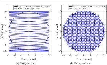
As the total acquisition time in our approach is limited by the steering mirror scanning speed, optimizing the scan patterns to cover all scanning point combinations as quickly as possible becomes critical. One steering mirror will be driven with a fast Lissajous figure, while the other steering mirror will cover the uncertainty cone with a slower hexagonal scan pattern, as shown in Figure 3.11. The Lissajous scan will have a 3 mrad amplitude and a fast-to-slow axis frequency ratio of ffast axis

fslow axis = 36 to give the required 2rwc grid spacing.

The centers between points in the hexagonal scan will also follow the required grid spacing and unlike the Lissajous pattern are evenly distributed over the total uncertainty cone area. The steering mirror with the hexagonal scan will dwell at each of its scan points long enough to allow the Lissajous steering mirror (on the other satellite) to cover its entire Ruc uncertainty space. Scanning over the 4 alignment degrees of freedom in the

commissioning scan with these parameters (when driving the fast-axis of the Lissajous near its estimated mechanical limit of 100 Hz) takes 214 seconds, and when combined with sweeping the laser frequency difference at a rate of 88 kHz/s over_±1 GHz, the entire commissioning sequence takes approximately 6.3 hours.

(38)

−3 −2 −1 0 1 2 3

−3

−2

−1 0 1 2 3

R uc = 3 mrad uncertainty cone 36-to-1 Lissa jous scan

Yawψ[mrad]

Pit

ch

θ

[mrad]

(a) Lissajous scan.

−3 −2 −1 0 1 2 3

R uc = 3 mrad uncertainty cone 595 scan points

Yawψ [mrad]

Pit

ch

θ

[mrad]

[image:38.595.51.479.82.343.2]

(b) Hexagonal scan.

Figure 3.11: Steering mirror scan patterns covering Ruc = 3 mrad with a maximum grid

spacing of 2rwc= 284µrad. (a) 36-to-1 Lissajous scan on steering mirror 1; (b) 595 point

hexagonal scan on steering mirror 2. The hexagonal steering mirror will dwell at each point in its scan long enough to allow the Lissajous steering mirror to cover an entireRuc

scan. During the spatial scanning, the frequency of the slave laser will be slowly swept, and the spatial scanning sequence will repeat until the entire frequency uncertainty range

func has been covered.

3.2.2 Reacquisition scan

To finalize the alignments, a reacquisition scan will be performed—a smaller, faster spatial and frequency scan—to confirm the commissioning results and optimize the pointing before transitioning to wavefront sensing-based alignment, and ultimately science operation. This reacquisition scan can potentially be utilized to automatically reacquire after a temporary loss of the laser link without intervention from the ground.

One approach for a reacquisition scan uses the same signal processing algorithms as for the commissioning scan on each satellite, but with reduced angular and frequency range (e.g. reducing Ruc and func, perhaps by a factor of 10). Another approach would be

to perform the reacquisition scans entirely on one satellite. For example, if the master laser dropped lock with its cavity, it would first re-lock to the cavity and steer its beam to the last best alignment point before the laser link was lost. The slave satellite would wait a fixed amount of time after the link was lost (to allow the master to re-lock to its cavity), then perform a fast spatial scan covering a 300µrad uncertainty cone with a more densely-packed pattern (decreased grid spacing). This finer scan performed only on the slave steering mirror could be enough to simultaneously increase the beat note amplitudes on each satellite. In our experiment, we adopted a hybrid between these, where each steering mirror scanned over a reduced angular uncertainty cone of 300µrad, but the grid spacing for only the Lissajous scan was reduced, from 2rwc = 284µrad to 28µrad. The

Inter-Satellite laser interferometry