Understanding spatial patterns in the production of multiple urban ecosystem services

Understanding spatial patterns in the production of multiple urban

ecosystem services

Alison R. Holt

, Meghann Mears, Lorraine Maltby, Philip Warren

Department of Animal and Plant Sciences, The University of Sheffield, Sheffield S10 2TN, UK

a r t i c l e i n f o

Article history: Received 26 March 2015 Received in revised form 20 August 2015 Accepted 21 August 2015

Keywords: Ecosystem services Mapping Spatial pattern Urbanisation Urban greenspace Urban planning

a b s t r a c t

Urbanisation is a key driver of land use change and urban growth is set to continue. The provision of ecosystem services depends on the existence of greenspace. Urban morphology is potentially an im-portant influence on ecosystem services. Therefore, it may be possible to promote service provision through an urban structure that supplies the processes and functions that underpin them. However, an understanding of the ability of urban areas to produce multiple ecosystem services, and the spatial pattern of their production, is required. We demonstrate an approach using easily accessible data, to generate maps of key urban ecosystem services for a case study city of Sheffield, UK. Urban greenspace with a mixture of land covers allowed areas of high production of multiple services in the city centre and edges. But crucially the detection of such‘hotspots’depended on the spatial resolution of the mapping unit. This shows there is potential to design cities to promote hotspots of production. We discuss how land cover type, its spatial location and how this relates to different suites of services, is key to promoting urban multifunctionality. Detecting trade-offs and synergies associated with particular urban designs will enable more informed decisions for achieving urban sustainability.

&2015 The Authors. Published by Elsevier B.V. This is an open access article under the CC BY license (http://creativecommons.org/licenses/by/4.0/).

1. Introduction

Urbanisation causes profound changes to natural systems (Grimm et al., 2008), and may result in a decline in ecosystem services – the benefits that humans derive from ecosystems (Millennium Ecosystem Assessment, 2005;Niemelä et al., 2010;

Tratalos et al., 2007). To adopt urban planning that can enhance ecosystem services requires an understanding of the spatial pat-tern of multiple ecosystem service production in and around cities. Urban ecosystems can provide a wide range of ecosystem services such as food supply, air purification, climate regulation (cooling), carbon sequestration, runoff mitigation and noise reduction, as well as recreational services and those that provide psycho-phy-sical and social health benefits (Bolund and Hunhammar, 1999;

Gómez-Baggethun and Barton, 2013;Niemelä et al., 2010). How-ever, the diversity and level of service provision depends largely on the green spaces that exist in and around urban areas, for in-stance road verges, cemeteries, allotments, gardens, parks and adjacent rural areas (Bastian et al., 2012).

The need to manage urban green spaces for services has be-come of policy importance at the UK and the EU level. For ex-ample, the UK Natural Environment White Paper (HM

Government, 2011) outlines a concern for the decline in the quality and quantity of urban greenspace in the UK, and recognises its role in reducing the risk offlooding and the heat island effect. The EU-wide strategy on Green Infrastructure (GI), Enhancing Europe’s Natural Capital (COM/2013/0249 final), identifies the importance of GI (a strategically planned network of green and blue spaces designed and managed to deliver a wide range of ecosystem services) in urban environments for providing health benefits through clean air and improved water quality. It also states that the consideration of GI is necessary in planning and decision-making processes to reduce the loss of ecosystem ser-vices as a consequence of land take (land that is converted for housing, industry, roads or recreation) and to help improve and restore soil functions.

Evidence is emerging to support the assertion that urban morphology (the biophysical structure of the urban environment, including green space, that is largely determined by urban plan-ning processes) may be an important factor influencing the pro-vision of multiple ecosystem services (Bierwagen, 2005; Kroll et al., 2012;Radford and James, 2013;Schneider et al., 2012; Tra-talos et al., 2007; Whitford et al., 2001). If this is so, the combi-nation of types and levels of ecosystem services produced could be optimised for particular circumstances through the creation of an urban morphology that enhances the environmental processes and functions that underpin them. However, such urban planning requires an understanding of the ability of urban areas to produce Contents lists available atScienceDirect

journal homepage:www.elsevier.com/locate/ecoser

Ecosystem Services

http://dx.doi.org/10.1016/j.ecoser.2015.08.007

2212-0416/&2015 The Authors. Published by Elsevier B.V. This is an open access article under the CC BY license (http://creativecommons.org/licenses/by/4.0/).

n_{Corresponding author.}

multiple ecosystem services, and the spatial pattern of multiple ecosystem service production in and around cities, of which there remains very little understanding (Haase et al., 2014).

Frameworks and methodologies have recently emerged that aim to assess ecosystem service provision and demand for urban and landscape scale planning (e.g.Bastian et al., 2012;Burkhard et al., 2012; Kopperoine et al., 2014; Koschke et al., 2012). But, accurate mapping of urban ecosystem service provision at differ-ent scales is necessary for effective spatial planning (UK NEA, 2011), and a better understanding of their trade-offs and re-lationships to land cover change is crucial (Haase et al., 2012,2014;

Lin and Fuller, 2013). The challenge remains the lack of accurate data with which to quantify ecosystem services or proxies of them (Naidoo et al., 2008;Seppelt et al., 2011;Wallace, 2007), particu-larly at the scales required for urban planning, management and policy-making. Indeed, most studies of this kind have mapped the supply of multiple ecosystem services at a much courser grain (global, continental, national and sub-national seeCrossman et al., 2013). Despite more recent studies atfiner scales (e.g.Vorstius and Spray, 2015) less is known about theflows of ecosystem services at local to regional scales (de Groot et al., 2010). There have been few attempts to quantify and map variation in ecosystem service provision across a city as a whole, and most have focused on single ecosystem services (Haase et al., 2014). In the absence of primary data at appropriate scales, the alternatives are the collection of the necessaryfield data and the use of ecological production functions. The former is resource intensive (Maes et al., 2012), even just for one ecosystem service, and for many practical applications, col-lection of significant newfield data is unlikely to be possible. It is important, therefore, to explore the utility and effectiveness of alternative approaches that can combine the use of field data where available with land cover and soils information, and other data likely to be readily available for urban areas (and therefore to urban planners), to generate maps of ecosystem service provision in urban systems.

In this paper, we demonstrate how multiple ecosystem services can be quantified using easily accessible/publically available data, to produce maps of a number of key ecosystem services in a large urban area: the city of Sheffield, UK. Importantly, this approach allows us to analyse the extent to which ecosystem services in

urban systems may co-occur and are correlated, and the simila-rities in spatial pattern of the levels of production between them. Furthermore we explore whether these patterns change depend-ing on the spatial unit at which the services are mapped. This enables an assessment of the extent to which urban ecosystem services may be managed and/or conserved together, whether it is possible to identify priority areas for creating hotspots of ecosys-tem service provision, and whether the unit at which services are mapped matters for decision-making.

2. Material and methods

2.1. Study area

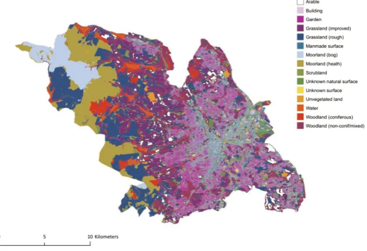
The city of Sheffield, (53°23′N, 1°28′W), is the ninth largest urban area in the UK (Fuller et al., 2008), with a human population of ca. 530,000 (Lovatt, 2007), in an area of 368 km2. Sheffield is hilly and lies over a wide altitudinal range, from 592 m above sea level in the west to 19 m a.s.l. in the east. There is a strong long-itudinal pattern in land cover and land use in Sheffield due to soils of loam and clay in the east and peat soils to the west, with blanket peat at higher altitudes (Cranfield University, 2009;Fine, 2003). Ninetyfive percent of the population live in the urbanised eastern part of the city (Beer, 2003). The west includes a sub-stantial area of the Peak District National Park (moorland and upland bogs), arable and pasture land interspersed with areas of woodland where the density of buildings is low (seeFig. 1).

We used the administrative boundary of the metropolitan borough of Shef_field as the study area because it is the unit most relevant to city-wide decision-making. Sheffield city is particularly suitable to this study as it (i) has an established and valued urban greenspace infrastructure, indicating that although management is not targeted at ecosystem services, they are indirectly valued, and (ii) the city boundary contains within it a number of broad eco-logical and environmental gradients giving rise to considerable variation in land use, land cover and thus the quality and quantity of ecosystem services produced.

2.2. Ecosystem services

A suite of ecosystem services were identified, chosen on the basis that they were likely to be of high priority to decision makers in an urban context, and that suitable models for each of them (or models that could be easily adapted) were available. The six eco-system services were (i) reduction of air pollution by vegetation, (ii) mitigation of the heat island effect by vegetation, (iii) reduction of storm water runoff through retention in soils and by vegetation, (iv) carbon storage in soils and vegetation, (v) opportunities for cultural ecosystem services (e.g. recreation and relaxation) in greenspace, and the (vi) provision of habitat forflora and fauna. These ecosystem services vary in the factors controlling their production and delivery, their spatial and temporal characteristics, and the type of benefits provided to humans. (seeTable SM1.3for a summary).

2.3. Spatial data

Three spatial data inputs were required for the ecosystem service models, a land cover map, a soil map (LANDis National Soil Map GIS dataset (NATMAP Vector)) and associated soil attribute data (SOILERIES and HORIZON data tables). The land cover map (Fig. 1, Table SM1.1) was made to suit the requirements of the study and was a combination of data from the level two vector version of the Land Cover Map 2000 (LCM 2000), and Ordnance Survey Mastermap (Ordnance Survey, 2008) topography layer. The resolution of the LCM2000 is low compared to the scale of land cover heterogeneity in densely urbanised areas, so the MasterMap topography layer was used to identify units of relatively homo-geneous land cover as a basis for land cover mapping. The topo-graphy area polygons were used to generate the land cover map polygons (each polygon was assigned to a single land cover type). However, there were some polygons for which it could not resolve a land cover type. For example, some polygons were classified as unknown, or a more speci_fic issue was that farmland was classi_fied as“general surface”. In these cases the LCM2000 was used to at-tempt to classify the polygon. To simplify the land cover data structure, and to facilitate integration with LCM2000 data (which only detects the tallest layer of vegetation from satellite imagery), the polygon was classified by the tallest layer of vegetation. Therefore, if a polygon included trees and scrub, the polygon was classified as having tree vegetation; or if it included scrub and grass, it was classified as scrub. The order of dominance was considered as follows: trees4scrub4heath/moorland4grass4

unvegetated. This land cover classification and typology were va-lidated by georeferencing aerial photography downloaded from Google Earth, and classifying the majority land cover within polygons by eye. The opportunities for cultural ecosystem services required an extra data source in the form of a land use map. The South Yorkshire Historic Environment Character Area (HECA) broad types classi_fication GIS layer was used for these purposes (seeTable SM1.2and below), in addition to using it simply as a spatial unit for mapping the modelled services (see below).

The modelled ecosystem services were mapped at three dif-ferent spatial units: 500 m grid squares (an arbitrary grid), Output Areas (OA) and HECA, in order to explore if the information on which mapping boundaries were delineated had implications for the modelled ecosystem service distribution. The OA boundaries were generated based on socioeconomic aspects of the resident population, following analysis of the UK 2001 Census data (see

http://www.ons.gov.uk/ons/guide-method/geography/beginner-s-guide/census/output-area–oas-/index.html). OAs consist of clus-ters of adjacent postcode areas, with social homogeneity de-termined from household tenure and dwelling type. The source of this dataset was the Office for National Statistics (2007) and

Vickers and Rees (2007). In contrast the HECA polygons signified areas of relatively homogeneous urban design, as they were based on areas identified as unique and characterised as one of twelve broad types, that include the date from which the current char-acter originated. The data were derived from the South Yorkshire Historic Environment Characterisation Project (South Yorkshire Archaeology Service, 2005, see〈http://sytimescapes.org.uk〉for full description). It is likely that decision-makers will map ecosystem services using spatial units that reflect the social and or environ-mental composition of a city rather than a uniform grid, therefore the consequences of such mapping should be investigated.

Initially, ecosystem services were modelled over the grid of 500 m500 m squares imposed within the boundaries of the unitary authority of Sheffield (derived from GIS data from the

Office for National Statistics, 2004). They were then, using means weighted by area, mapped at the OA and HECA spatial units. Each of the three spatial unit maps were clipped to the boundaries of the Sheffield unitary authority, with small fragments of polygons at the very edge of the area (presumed to be mostly outside of Sheffield) identified by eye and excluded from analyses. All GIS analyses were carried out in ARCGIS/ARCINFO 10 (ESRI, Redlands, CA, USA).

2.4. Spatially explicit ecosystem service models

Ecosystem service models were based on existing models that could be used, or adapted for use, in combination with the study area data on land cover, and land use to enable production func-tions to be calculated. In deriving estimates of the various eco-system services, our primary interest was to identify the additional service generated by the urban greenspace infrastructure, when compared to the non-green alternative, i.e. an entirely built en-vironment. So, for example we are interested in the difference in pollutant removal between the urban environment with green-space in it and the same area with the greengreen-space replaced by non-green (built) urban surfaces. The reason for this is that

arti-ficial surfaces will also influence the particular processes under-lying the services we are interested in, particularly in the case of storm water run-off, reduction of air pollution and carbon storage. For example, they can provide deposition surfaces for pollutants (Zhang et al., 2003), abstract small amounts of storm water ( USDA-NRCS, 1986) and urban soils can contain a substantial amount of organic carbon beneath impervious surfaces (Edmondson et al., 2012).

The ecosystem services of reduction of air pollution, heat island mitigation, storm water runoff reduction, carbon storage modelled were, therefore, quantified and mapped as the difference between the level of service (e.g. amount of air pollution reduced) that occurs given the actual land cover composition (including green space), and the level of service that would occur if the whole area were composed of 28% buildings and 72% other manmade surfaces (a hypothetical scenario replacing the current levels of greenspace with buildings and manmade surfaces to the same proportions as existing artificial surface areas of the city). Neither the opportu-nities for cultural services nor habitat provision for biodiversity were compared to a hypothetical land cover as the modelling was based on proportion of the area that is suitable for providing the services. That is, if greenspace did not exist the level of these services would be zero.

2.4.1. Reduction of air pollution

The air pollution reduction model focuses on the amount of pollution removed over and above that which would be removed in the absence of the greenspace infrastructure for Sheffield's two most problematic pollutants: nitrogen dioxide (NO2) and

2009;Sheffield City Council, 2008a,b). The potential production of air pollution reduction is either the capacity of plant and ground surfaces to intercept pollutants or the inverse of the resistance to deposition or the deposition velocity. The actual production of the ecosystem service is also dependent on how the interception ca-pacity is used, which is determined by the local levels of air pol-lution. Inputs to the model comprised land cover (e.g. total leaf area index, characteristic radius of particle collectors, derived by matching the general land cover typology for the study area to

Zhang et al. (2001,2002 and 2003)), meteorological and pollutant concentration data, as well as a number of empirical parameters such as process rates and constants. These data were used to es-timate the deposition velocity,Vd, of the pollutants to the different types of land cover found in the study area. The estimates were then superimposed on the land cover map and an average calcu-lated across each 500 m grid square. This was also the spatial re-solution of the estimates of pollutant concentration,C, from the Sheffield City Council’s AIRVIRO model. These two inputs were used to calculate the totalflux of pollutant deposition to the land covers,F, for each 500 m grid square, asF¼VdC.

A second estimate ofFwas made assuming that all land cover was artificial, i.e. no ecosystem service was being produced. The

first estimate (from the land cover map) was then divided by the second (assuming no natural land covers) to calculate the eco-system service provided by the presence of natural land covers, and the monthly _figures averaged to produce a single annual average for each pollutant. Thefigures were divided rather than subtracted in order to give equal weighting to the two pollutants, concentrations of which occur over different orders of magnitude. Finally, the mean of these twofigures was taken to generate a single index of ecosystem service production for each 500 m grid square area. The land cover composition of each polygon in the OA and HECA maps was used to calculate the deposition velocity, and was multiplied by the area-weighted mean (derived from the 500 m grid squares) pollutant concentration to calculate the pol-lutant_flux according to the equation above.

2.4.2. Heat island mitigation

Heat island mitigation is quanti_fied here as the reduction in surface temperature that results from the presence of greenspace in the land cover matrix, i.e. the difference between the tem-peratures modelled for the actual land cover and the hypothetical scenario in which no greenspace is present. We used the urban climate model developed byTso et al. (1991)that has been applied to towns and cities in the UK (seeGill, 2006;Tratalos et al., 2007;

Whitford et al., 2001). Surface temperatures were used as they determine the mean radiant temperature, which is a dominant factor contributing to human comfort levels (Gill, 2006; Matzar-akis et al., 1999), and are more reliable when estimating tem-peratures from a known surface composition over large scales (Whitford et al., 2001). The model estimates the maximum day-time surface temperature for a given set of meteorological para-meters, customised to represent an extremely hot summer day in Sheffield (29.23°C, the mean maximum temperature of the hottest day of each year from 1999 to 2008 (data from the UK Meteor-ological Office). Spatially variable model inputs included land cover and soil properties. The model is based on a traditional energy exchange equation, with an additional term to represent heat storage in buildings. This equation relates the heat storage in buildings,M, to the net radiationflux,R; the sensible heatflux to the air,H; the latent heat of water,L; the evaporation rate,E; and the heat flux to the soil substrate, G Tso et al. (1991) as

M¼RHL E G. The model estimates the temperature at ground level and in the soil layer during the course of 24 h (Gill, 2006), and the temperature for each cell in the grid of 500 m500 m squares superimposed over the study area. The

maximum temperature during the modelled 24 h period was re-corded, and from this value the estimated temperature for the hypothetical land cover was subtracted. The result of this sub-traction quantifies the production of the ecosystem service of heat island mitigation.

2.4.3. Storm water runoff reduction

Urbanisation replaces natural land covers with developed and often impermeable surfaces such as buildings and roads (Kline, 2006;USDA-NRCS, 1986). This reduces the amount of precipitation that is intercepted and later evapotranspired by vegetation, and that which infiltrates and is stored in the soil, greatly increasing surfaceflow (Booth et al., 2006;Whitford et al., 2001). The storm water runoff reduction model calculated the ability of the green-space to abstract more water than the hypothetical scenario using the curve number method to estimate surface runoff following a storm event (USDA-NRCS, 1986,Whitford et al., 2001):

⎧ ⎨ ⎪

⎩ ⎪ Q

P S

P S P S

P S

0.2

0.8 , if 0.2

0, if 0.2 1 2

=

( − ) + >

≤ ( )

S CN 2540

25.4

2 = −

( )

whereQ is the runoff depth (in cm),Pis the precipitation (cm),

Sis the maximum potential retention once runoff begins, andCN

is the curve number for a particular combination of land cover type, soil hydrological group (a categorisation of soil type based on infiltration rates, which is strongly related to soil texture) and antecedent soil moisture conditions (a categorisation of how dry or wet the soil is before the scenario precipitation event).

When applied to a specified precipitation scenario, the curve number can calculate the proportion of precipitation that runs off as surfaceflow (USDA-NRCS, 1986). The curve number method is suitable for application in urban areas (USDA-NRCS, 1986), and has previously been implemented in similar studies byWhitford et al. (2001)andTratalos et al. (2007). The model uses the land cover map and soils map (and associated soil texture data) as input. Curve numbers were assigned from lists given in a USDA-NRCS technical report (USDA-NRCS, 1986), using previous implementa-tions byWhitford et al. (2001)andTratalos et al. (2007) as gui-dance. Two rainfall event scenarios were designed: a‘typical heavy rainfall’scenario, representing a fairly common event in Sheffield, with 1.2 cm rainfall and soils not especially wet due to recent rainfall; and an‘extreme rainfall’event, based on the June 2007 rainfall that caused extensive flooding in Sheffield, with 6 cm rainfall onto already saturated soils. For each scenario, the runoff volume per m2was spatially assigned according to the land cover and soils maps, and from this value was subtracted the runoff that would have occurred if each m2 _{was covered by artificial,}

im-pervious surfaces. This calculated the reduction in runoff due to natural land covers. Ecosystem service production was calculated as the average reduction in runoff from the two scenarios.

2.4.4. Carbon storage

⎡ ⎣ ⎢ ⎢ ⎛ ⎝ ⎜ ⎜ ⎞ ⎠ ⎟ ⎟ ⎤ ⎦ ⎥ ⎥ x a a storage per area

3 j n ij ij j n ij 1 1

∑

Where the subscriptxijis the carbon storage value for all land cover map polygonsiof a land cover categoryj, andaijis the area, such that a

a ij j n ij 1 ∑=

is the proportional abundance of a land cover

category.

Soils under manmade surfaces and buildings were assumed to have half the carbon content that they would otherwise, because the development process generally causes large losses of carbon (Pouyat et al., 2006) (although there is now emerging evidence that existing assumptions about urban soil carbon may be open to question, see (Edmondson et al., 2012)). Soil carbon losses can occur during development regardless of whether the soil is di-rectly disturbed or not, due to the loss of plant, microbial and earthworm biomass, which reduces inputs of organic matter (the source of carbon) to the soil (Byrne et al., 2008). Direct disturbance can also expose the deeper soil layer to conditions in which carbon is likely to oxidise to the atmosphere (Jandl et al., 2007). To quantify the ecosystem service provided by natural land covers, an estimate was also made of the carbon content of the different soil types when under sealed surfaces. This second estimate was subtracted from thefigure for actual carbon storage. Carbon sto-rage in soils, or specifically organic carbon (estimates of inorganic carbon were not available) is estimated using a similar approach, using soil and horizon specific estimates of organic carbon by weight and bulk density to calculate the carbon per unit area of a soil map polygon:

⎡ ⎣ ⎢ ⎢ ⎛ ⎝ ⎜ ⎞ ⎠ ⎟⎤ ⎦ ⎥ ⎥ C

B H S carbon storage g m

100 100 10 ₄ j

n

i n

ij ij ij j 2 1 1 4

∑ ∑

WhereCis the percent of carbon by weight in horizoniof a soil series j (there are multiple soil series within any one soil map polygon),Bis the bulk density of the soil series in g cm3,His the soil horizon depth in cm, S is the percentage of the soil map polygon composed of the soil series and 104converts the estimate from 1 cm2to 1 m2. An area weighted mean of the polygon esti-mates for a speci_fic area of interest can then be made using Eq. (3), where the subscripts are the soil map polygonsiof a particular soil type j. A total estimate of carbon storage was made by adding the vegetation and soil estimates.

2.4.5. Opportunities for cultural ecosystem services in public greenspaces

The model of access to opportunities for cultural ecosystem services in greenspace describes the spatial availability of green-space infrastructure to the general public. The production of op-portunities is calculated as the proportion of an area of interest that is covered by land uses that are considered to provide such opportunities (e.g. public parks, moorland, woodlands). The supply of opportunities was quantified using the four distance-related greenspace provision standards (seeHandley et al., 2003). Areas of publicly accessible greenspace were identified from the HECA dataset. The land use map legend (Fig. 1) was studied in order to identify whether areas of each category were likely to fulfil two requirements: (i) that greenspace is a major component of that land use; and (ii) that the greenspace is freely publicly accessible.

Table SM2.1shows the land use categories that were considered to meet these requirements. These areas were identified on the land use map and used to generate a map of publicly accessible greenspace. The proportion of each area of interest meeting each of the standards was calculated, i.e. within 300 m of a 2 ha greenspace, 2 km of a 10 ha greenspace, 5 km of a 100 ha

greenspace and 10 km of a 500 ha greenspace (Handley et al., 2003). These proportions were summed and divided by four in order to calculate an index quantifying this ecosystem service. Areas of greenspace located only partially within, or nearby to the boundaries of the study area were also included in generating these proportions.

2.4.6. Provision of habitat for biodiversity

Biodiversity is thought to be critical to the production of many ecosystem processes, services and benefits (Cardinale et al., 2012;

Mace et al., 2011). Due to a lack of consistent and reliable records of biodiversity at the scale required for the study area, we devel-oped a land cover-based metric for ecosystem service providing biodiversity. It describes the degree of urbanisation and the variety of remnant natural habitats, similar to that of Whitford et al. (2001). Urban development increases impermeable surfaces, splitting the natural vegetation into smaller patches that may have low connectivity (Bolger et al., 2000;Crooks, 2002). Greenspace management by gardeners and landscape architects means that the remaining natural vegetation may also be converted to dif-ferent types of land cover, changing the availability of some types of habitat (McKinney, 2006). Given this, three metrics, proportion of area comprising of natural land covers, habitat diversity and natural land cover patch connectivity, were chosen to reflect dif-ferent components of these complex effects. Thefirst metric is the proportion of the area of interest that is covered by natural land covers. Habitat diversity was calculated using the Shannon di-versity index H′(Whitford et al., 2001):

H plogp

5 i k i i 1 2

(

)

∑

where pi are the proportions of each habitat type andkis the

number of habitat types present in the area of interest. Unknown surfaces and unknown natural surfaces were excluded from the calculation ofH′. However, manmade surfaces and buildings were included as a single habitat type, because some species thrive in close association with humans (McKinney, 2006). In order to have metrics with the same numerical range,H′was then scaled by the maximum possible value that would exist if all possible land covers were present in exactly equal proportions. The correlation length, also known as the area-weighted mean radius of gyration, is used to represent the connectivity of individual patches of natural land cover through their average size. Connectivity is portant because habitat fragmentation is thought to be an im-portant cause of the loss of some species from urban areas (Bolger et al. 2000, Crooks 2002). The radius of gyration is sensitive to shape as well as area: for two patches of equal area, the less cir-cular will have a higher radius of gyration. In the present context, it can be interpreted as a measure of the average distance in which a mobile organism confined to natural land cover can travel in an area of interest, from a random starting point, before reaching intraversible land. The radius of gyrationGof each area of natural land cover (any except buildings, manmade surfaces, unknown surfaces–but not unknown natural surfaces–and water) is cal-culated on a cell-by-cell basis within each patch of natural land cover as follows:

G h z ₆ i j z ij 1

∑

where hij is the distance (m) between cell j located within patch iand the centroid of patch i, and zis the number of cells within patchi.Gis in units of metres. The area-weighted meanG¯

⎡

⎣ ⎢ ⎢

⎛ ⎝ ⎜⎜ ⎞

⎠ ⎟⎟⎤

⎦ ⎥ ⎥

G G a

a ₇

i n

i i

i n

i

1 1

∑

¯ =

∑ _{( )}

= =

where ai is the area of patch i and nis the total number of patches. To account for differences in sizes of areas of interest,G¯ _is

then scaled to the maximum possible value ofG¯ _{if that area}

con-tained only natural land cover. However, if the area of interest contains patches of highly irregular shape, or is itself irregularly shaped, the land cover rasterisation methods used means it is occasionally possible for the scaled value to be greater than one; in these cases, a value of exactly one is assigned. All the metrics were computed using FRAGSTATS software (McGarigal et al., 2002).

They were then averaged to produce an index of habitat provision (seeSM2.3andFig. SM2.3for the calculation of each of the metrics and their asscoaited maps).

2.5. Analyses

Statistical analyses were carried out in R 2.14.1 (R Development Core Team, 2011). Spearman’srhorank correlations were used to quantify the degree of association between pairs of ecosystem services at each spatial unit (500 m grid squares, OA and HECA) as data were non-normal in distribution. Bonferroni corrections (Holm, 1979) were used due to multiple comparisons within the same data set. We used the Bonferroni probability threshold of

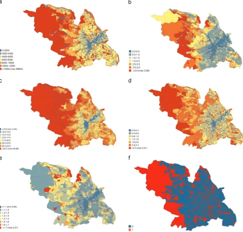
Fig. 2.(a) The ecosystem service of carbon storage (g m2

) aggregated to Historic Environment Character area boundaries. (b) Reduction of storm water run off (cm depth) aggregated to Historic EnvironmentCharacter area boundaries. (c) Heat island mitigation (°C) aggregated to Historic Environment Character areaboundaries. (d) Index of habitat forflora and fauna (average of proportion of area comprising of natural land covers, habitat diversity and natural land cover patch connectivity metrics) aggregated to Historic Environment Character area boundaries. (e) Air pollution reduction (pollutantflux to surfacesμg m2

s1

0.0002 as the corrected threshold equivalent of 0.001, the con-servative level to account for the fact that spatial statistics were not being used (as there is currently no straightforward option for dealing with spatial autocorrelation in data that is non-normal (seeEigenbrod et al., 2010)). Hotspots of service provision for each ecosystem service were calculated following Anderson et al. (2009). We used two thresholds, the top 10% and 25% of polygons with the highest ecosystem service values. These were used to

determine the number of ecosystem services for which each polygon, at each of the three spatial units, across the study area, is a hotspot. This was used to develop an understanding of the spatial covariance of ecosystem services by calculating the hotspot overlap (the number of ecosystem services for which each polygon is a hotspot), and the pair-wise co-occurrence of ecosystem service hotpots (the proportion of all polygons that are hotspots for two specific ecosystem services).

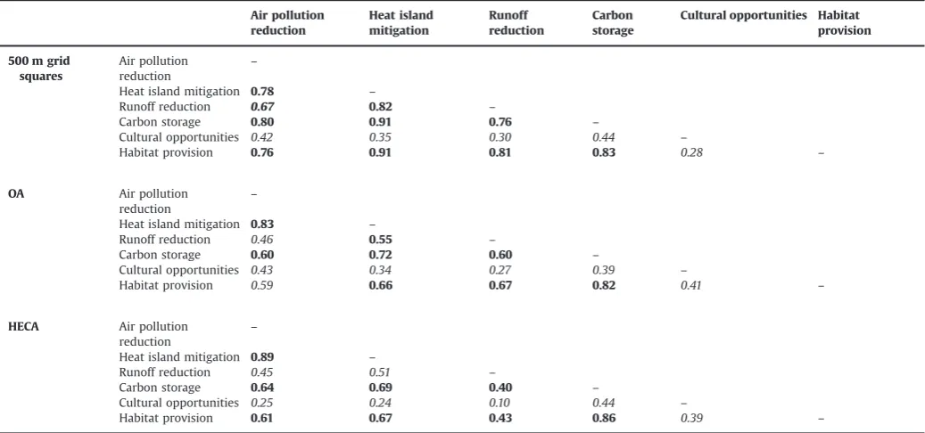
Table 1

Spearman’s rank correlation coefficient matrix for ecosystem services assessed over three spatial units of analysis. Bold values indicate strong correlations while italic values indicate weak correlations. Roman values indicate that the result is taken to be statistically non-significant, regardless of whether the Bonferroni corrected threshold is used (none are significant only at one threshold).

Air pollution reduction

Heat island mitigation

Runoff reduction

Carbon storage

Cultural opportunities Habitat provision

500 m grid squares

Air pollution reduction

–

Heat island mitigation 0.18 –

Runoff reduction 0.20 0.69 –

Carbon storage 0.20 0.92 0.67 –

Cultural opportunities 0.03 0.72 0.48 0.73 –

Habitat provision 0.52 0.65 0.62 0.60 0.33 –

OA Air pollution

reduction

–

Heat island mitigation 0.83 –

Runoff reduction 0.47 0.55 –

Carbon storage 0.61 0.72 0.60 –

Cultural opportunities 0.44 0.34 0.28 0.40 –

Habitat provision 0.59 0.66 0.67 0.82 0.42 –

HECA Air pollution

reduction

–

Heat island mitigation 0.89 –

Runoff reduction 0.64 0.71 –

Carbon storage 0.65 0.70 0.86 –

Cultural opportunities 0.28 0.28 0.40 0.44 –

Habitat provision 0.63 0.70 0.85 0.85 0.40 –

Table 2

Spearman's rank correlation coefficient matrix for ecosystem services assessed over three spatial units of analysis, for the urban area of Sheffield only. Bold values indicate strong correlations while italic values indicates weak correlations. Roman values indicate that the result is taken to be statistically non-significant.

Air pollution reduction

Heat island mitigation

Runoff reduction

Carbon storage

Cultural opportunities Habitat provision

500 m grid squares

Air pollution reduction

–

Heat island mitigation 0.78 –

Runoff reduction 0.67 0.82 –

Carbon storage 0.80 0.91 0.76 –

Cultural opportunities 0.42 0.35 0.30 0.44 –

Habitat provision 0.76 0.91 0.81 0.83 0.28 –

OA Air pollution

reduction

–

Heat island mitigation 0.83 –

Runoff reduction 0.46 0.55 –

Carbon storage 0.60 0.72 0.60 –

Cultural opportunities 0.43 0.34 0.27 0.39 –

Habitat provision 0.59 0.66 0.67 0.82 0.41 –

HECA Air pollution

reduction

–

Heat island mitigation 0.89 –

Runoff reduction 0.45 0.51 –

Carbon storage 0.64 0.69 0.40 –

Cultural opportunities 0.25 0.24 0.10 0.44 –

In order to understand how much difference the inclusion of the large rural area to the west of the city made to the spatial co-variation and hotspots of service provision, the analyses were re-peated for the ecosystem services at each spatial unit mapped for the predominantly urban area of Sheffield only, in which the majority of the human population live. A map, created following the definition of urban Sheffield used inDavies et al. (2008), was taken as a template to clip the metropolitan borough maps at each spatial scale for each ecosystem service, and polygons were ac-cepted as part of the urban area if they contained Z25% urban land use. Urban Sheffield was defined by the boundaries of

Shef-field city and the borough of Rotherham to the east, by the Der-byshire/South Yorkshire county border to the south, the north and west was defined by assigning 11 km2_{grid squares having more}

or less than 25% coverage of industrial and residential land use.

3. Results

The single ecosystem service maps (Fig. 2(a)–(f)) for services mapped at the HECA unit, and seeFig. SM3.1-12for maps at 500 m grid square and OA units) show a general trend for ecosystem service production to increase with distance from the city centre. However, the reduction of air pollution service is an exception (Fig. 2(a)–(f),SM3.1-12). Despite this general tendency, there is variation in the levels of service production in the urban centre, with fragments of low, moderate and high ecosystem service production. The HECA and OA spatial units show more variation in service production within the urban centre than the 500 m grid

square maps (Fig. 2(a)–(f),SM3.1-12).

3.1. The association between ecosystem services

The six services mapped within the metropolitan borough of Sheffield show positive associations, and all these, except the re-duction of air pollution and opportunities for cultural ecosystem services for 500 m grid squares (rho¼0.03) are statistically sig-nificant (Table 1). This shows that the six services have similar patterns of variation in production across the study area. However, whilst the associations remain positive, their strength differs de-pending on whether they have been mapped at 500 m grid squares, the OA or the HECA spatial units. For 500 m grid squares, there are strong associations (rhoZ0.33) between heat island mitigation, reduction of stormwater runoff, carbon storage, cul-tural ecosystem services and habitat provision. Those between the same ecosystem services and air pollution reduction are weaker (rhor0.2 except with habitat provision). Mapping the same ser-vices at the OA and HECA scales shows associations between all pairs of ecosystem services are at least moderately strong (rhoZ0.40), except with opportunities for cultural ecosystem services (rhor0.44). For these spatial units, unlike the 500 m grid squares, associations between the services and air pollution re-duction are only very slightly weaker than between other eco-system services.

Considering only the urban area of Sheffield, services showed similar patterns of variation in the level of production, as they did considering the whole metropolitan borough (Table 2). However, for the 500 m grid squares all associations were significant and in most cases much stronger, particularly between the air pollution reduction service and all other services, and between cultural opportunities and heat island mitigation, runoff reduction and carbon storage (Table 2). There was little change in the pattern of variation in the level of production between the services for the OA and HECA (Table 2). Removing the polygons in the largely rural component of the metropolitan borough from the analyses re-duced the disparity between the service associations of 500 m grid squares, OA and HECA spatial units. However, the associations between services in the OA and HECA spatial units still remained slightly more similar.

Table 3

Proportion of spatial units that are hotspots for multiple ecosystem services. Table entries indicate the proportion of spatial unit polygons that are a hotspot for the number of ecosystem services given in the column heading, where hotspots are defined as the top 10% of polygons for a given ecosystem service. Bold values in-dicate high proportions while italic values inin-dicate low proportions.

Top 10%

Number of ecosystem services 0 1 2 3 4 5 6

500 m grid squares 0.59 0.19 0.11 0.07 0.04 0.00 0.00

OA 0.72 0.13 0.06 0.03 0.04 0.01 0.00

HECA 0.73 0.12 0.07 0.04 0.03 0.02 0.01

3.2. Multiple service hotspots

A significant proportion of the metropolitan borough of

Shef-field supports high levels of production for between 1 and 6 eco-system services. Twenty eight to 41% of polygons, using the 10%

threshold, were hotspots for at least one ecosystem service ( Ta-ble 3,Fig. 3). Just over a third of this proportion of polygons sup-ports a high level of production for single ecosystem services (10% threshold: 43–46% of hotspot polygons, or 13–19% of the total number of polygons), with only a small proportion of this sup-porting high production of more than three ecosystem services at a time (10% threshold: 6%, regardless of the spatial unit at which they were mapped).

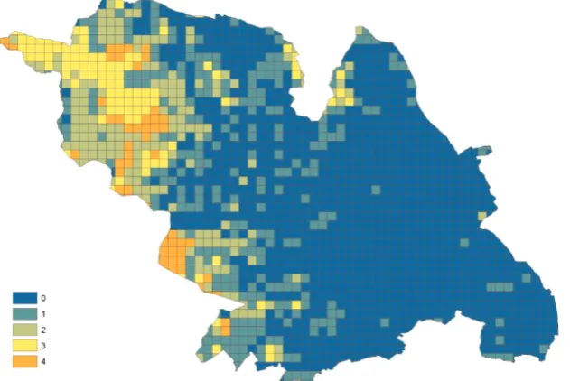
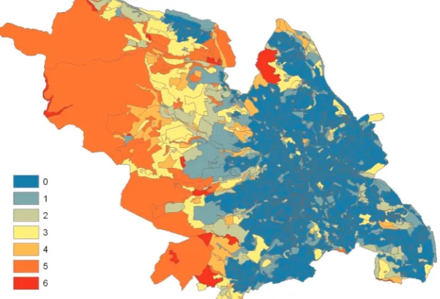
The distribution of hotspots within the metropolitan borough, when mapped at 500 m grid squares, is slightly different to that of the OA and HECA units, the latter two being more similar. This is particularly evident from the hotspots maps at the 10% threshold (Figs. 3–5). For the 500 m grid squares (Fig. 3), hotspots of more than three ecosystem services were mainly found in the west of the study area, a large proportion of the urban area supporting either no, or single service hotspots. At the OA and HECA units (Figs. 4 and 5) this is not the case. The smaller polygons in the

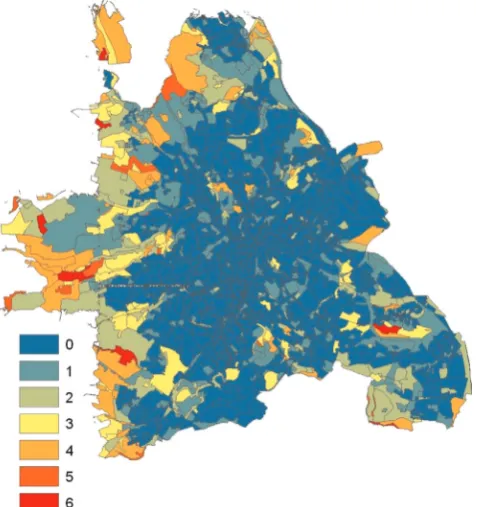
Fig. 4.Number of ecosystem services for which each Output Area is a hotspot. Hotspots are polygons in the top 10% of values for each ecosystem service.

Fig. 5.Number of ecosystem services for which each Historic Environment Character Area is a hotspot. Hotspots are polygons in the top 10% of values for each ecosystem service.

Table 4

Proportion of spatial units that are hotspots for multiple ecosystem services for the urban area of Sheffield only. Table entries indicate the proportion of spatial unit polygons that are a hotspot for the number of ecosystem services given in the column heading, where hotspots are defined as the top 10%. Bold values indicate high proportions while italic values indicate low proportions.

Top 10%

Number of ecosystem services 0 1 2 3 4 5 6

500 m grid squares 0.73 0.12 0.05 0.03 0.03 0.02 0.01

OA 0.72 0.14 0.05 0.04 0.04 0.02 0.00

urban area have revealed hotspots for three or more services, even 6 services in the urban south-east of the study for the OA unit, although a large proportion of this area still does not support high ecosystem service production. When the proportion of spatial units that are hotspots for multiple ecosystem services in urban Sheffield only were mapped, there was little difference in the re-sults for OAs using the 10% threshold, compared to the maps of the whole metropolitan borough (Table 4). However, there were some differences in the proportions in HECA and 500 m grid squares. In the case of the latter most notably the proportion of polygons that did not support any services increased, but there was also a slight

increase in polygons that supported high levels of production of 5 and 6 services simultaneously. The opposite was true for the HECA unit, the proportion of polygons that did not support any services decreased, and the number that supported 5 and 6 de-creased. All three spatial units now showed more similar propor-tions (Table 4). When viewing the hotspot maps (Figs.6–8) for the urban area only, the differences between the 500 m grid squares and the OA and HECA look pronounced. In the 500 m grid squares a larger proportion of the urban area (as opposed to the proportion of polygons) seems not to produce any ecosystem services to a high level (apart from at the urban fringes to the north west and

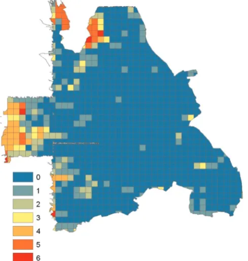
Fig. 6.Number of ecosystem services for which each 500 m grid square is a hotspot, for the urban area of Sheffield only. Hotspots are polygons in the top 10% of values for each ecosystem service.

west). This is in contrast to the more fragmented appearance of the blue area in HECA and OA maps (Figs. 6–8).

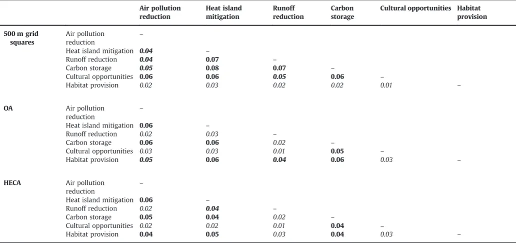
There was a tendency for certain services to occur together in hotspots (Table 5). Heat island mitigation, carbon storage and cultural opportunities co-occurred with each other as hotpots in 8–11% of polygons in the 500 m grid square unit at the 10% threshold. Runoff reduction and cultural opportunities was also one of the highest proportions among the services (9%). In OA and HECA maps co-occurrences were once again similar to each other, but quite different from 500 m grid squares. There were co-oc-currences between most ecosystem services (Table 5) at slightly lower proportions. When considering the urban area only, the trends in the results are very similar. However, the co-occurrence of hotpots for air pollution reduction with all other services were more pronounced. The OA and HECA spatial scales show no dif-ferences when compared to the whole metropolitan borough, but again show slightly different trends to the 500 m grid squares (Table 6), although this is now less marked.

4. Discussion

We have modelled multiple ecosystem service production in an urban system using readily accessible data sources, and this re-veals considerable variation in service production, and relation-ships between ecosystem services, across an urban system. There will inevitably be uncertainties associated with this type of ana-lysis (as discussed inHaase et al., 2012, see Supplementary ma-terial 2.1) through the use of land cover maps and the develop-ment of models that act as proxies for ecosystem services. To limit this we ensured that we validated the land cover classification by comparing the map to the most recent aerial photography of the area (see 2.3 Spatial data). Some ecosystem service models may also be more accurate than others. Air pollution reduction, heat island mitigation and stormwater runoff reduction are all

quanti-fied from process-based models of varying complexity (air pollu-tion reducpollu-tion being the most complex and runoff reducpollu-tion being

the least). The use of empirical parameters with unknown degrees of uncertainty or variability introduces some inaccuracy to the output from these models, however, they are based on well un-derstood science. We aimed to strike a balance between a greater potential reliability, resolution and data demand of more complex single service models and exploring the pattern of pro-duction across a greater breadth of ecosystem services. Indeed, the models such as heat island mitigation and stormwater runoff re-duction in this study are good examples of models whose im-plementation and use is sufficiently tractable as to make them viable for practical use in urban planning and policy. It also makes this study one of very few focused on the spatial distribution of multiple ecosystem services in an urban system (Haase et al., 2014), indeed of multiple ecosystem services in any context (Seppelt et al., 2011).

We found that individually the spatial pattern of provision of key urban ecosystem services showed their own distinct patterns (Fig. 2(a)–(f) andSM3.1-12). However, there was a general ten-dency for the production of ecosystem services to be high or low in the same places, with some of these coefficient values being quite high. For example, in this study the heat island mitigation, stormwater run off reduction, carbon storage and provision of habitat for biodiversity services had a strong association with each other over the different mapping units. This is likely to be because all these services require areas of natural, vegetated land cover to achieve high production levels. A similar trend was observed in

Haase et al. (2012), a temporal and spatial analysis offive urban ecosystem services, where synergies were also found between similar combinations of services (e.g. biodiversity potential, carbon storage and climate regulation). Where studies have looked for associations between ecosystem services they have quite often found low or negative correlations (e.g.Chan et al., 2006; Raud-sepp-Hearne et al., 2010). However, these studies have generally been measured over a greater spatial extent, at courser resolutions and across very different ecosystem services. In comparison, we have quantified ecosystem services at a much finer resolution. Here, where associations are weaker (e.g. reduction of air pollution

and cultural services) services do not show the same increasing production gradient outwards from the urban centre.

A keyfinding is that green space allows areas of high produc-tion (hotspots) of multiple services in both the urban centre and rural fringes of the city. High levels of ecosystem service produc-tion for single services can be supported, and commonly up to 3 services simultaneously. Areas that are hotspots for over 3 ser-vices occupy the more rural areas, but there are pockets in the urban centre, which are revealed when mapped using

environmental characteristics or local socio-economic factors as delineations. These tended to represent land uses such as parks, which contain a matrix of land covers that produce high levels of ecosystem services. Areas that were able to provide all 6 services were mainly woodland habitats on the edges of the city or the suburbs. Many studies have shown the importance of urban greenspace for maintaining both ecosystem and human health (e.g.Andersson et al., 2014;Cameron et al., 2012;Dallimer et al., 2012;Tzoulas et al., 2007). Our study reinforces the importance of

Table 5

Pairwise overlap in ecosystem service hotspots, with hotspots defined as the top 10% of polygons for a given ecosystem service. Table entries show the proportion of spatial unit polygons that are a hotspot for both the ecosystem services listed in the column and row headers. Bold values indicate high proportions while italic values indicate low proportions.

Air pollution reduction

Heat island mitigation

Runoff reduction

Carbon storage

Cultural opportunities Habitat provision

500 m grid squares

Air pollution reduction

–

Heat island mitigation 0.00 –

Runoff reduction 0.02 0.03 –

Carbon storage 0.00 0.08 0.04 –

Cultural opportunities 0.03 0.11 0.08 0.09 –

Habitat provision 0.02 0.00 0.01 0.00 0.01 –

OA Air pollution

reduction

–

Heat island mitigation 0.05 –

Runoff reduction 0.02 0.04 –

Carbon storage 0.06 0.06 0.02 –

Cultural opportunities 0.03 0.03 0.01 0.05 –

Habitat provision 0.04 0.06 0.04 0.06 0.03 –

HECA Air pollution

reduction

–

Heat island mitigation 0.05 –

Runoff reduction 0.04 0.06 –

Carbon storage 0.05 0.04 0.05 –

Cultural opportunities 0.03 0.03 0.03 0.04 –

Habitat provision 0.04 0.04 0.05 0.04 0.03 –

Table 6

Pairwise overlap in ecosystem service hotspots, with hotspots defined as the top 10% of polygons for a given ecosystem service, for the urban area of Sheffield only. Table entries show the proportion of spatial unit polygons that are a hotspot for both the ecosystem services listed in the column and row headers. Bold values indicate high proportions while italic values indicate low proportions.

Air pollution reduction

Heat island mitigation

Runoff reduction

Carbon storage

Cultural opportunities Habitat provision

500 m grid squares

Air pollution reduction

–

Heat island mitigation 0.04 –

Runoff reduction 0.04 0.07 –

Carbon storage 0.05 0.08 0.07 –

Cultural opportunities 0.06 0.06 0.05 0.06 –

Habitat provision 0.02 0.03 0.02 0.02 0.01 –

OA Air pollution

reduction

–

Heat island mitigation 0.06 –

Runoff reduction 0.02 0.03 –

Carbon storage 0.06 0.06 0.02 –

Cultural opportunities 0.03 0.03 0.01 0.05 –

Habitat provision 0.05 0.06 0.04 0.06 0.03 –

HECA Air pollution

reduction

–

Heat island mitigation 0.06 –

Runoff reduction 0.02 0.04 –

Carbon storage 0.05 0.04 0.02 –

Cultural opportunities 0.02 0.02 0.01 0.04 –

urban greenspace for providing multiple services. It begins to re-veal how greenspace, as a mosaic of different land covers, can produce bundles of ecosystem services. However, it is not only the land cover composition of greenspace that is important, but also its spatial location. For instance, a land cover will only provide important recreation and well-being enhancing services if it is physically accessible to people. The same combination of land covers that produce the heat island mitigation service in an urban system will be redundant in a rural landscape. This is particularly important in the context of the EU greening policies (COM/2013/ 0249final). How services co-vary (or not), and how land cover and its spatial location influences service level and production is cri-tical to creating city networks delivering a broad range of eco-system services for human well-being.

This study also revealed that the detection of ecosystem service hotspots is dependent on how services are mapped, in particular, on the spatial resolution of the mapping unit. We obtained con-sistently different results by using three distinct spatial units of analysis. The different spatial units represent fundamentally dif-ferent aspects of the system, and the fact that the choice of units has profoundly affected the conclusions drawn means that it is critical to choose a method of delineating spatial areas that is appropriate to the question or management decision of interest. For example, should a decision require an understanding of how altering urban form may influence ecosystem service production, boundaries similar to the HECA would be ideal as they delineate areas of relatively homogeneous land use, and by extension urban morphology. If a management decision requires knowledge about the relationship between the location of particular social groups and ecosystem service production, then a spatial unit that re-presents certain socioeconomic aspects of the resident population, such as OAs, would be much better suited.

5. Conclusions

This work suggests that there is a potential to design cities to encompass areas of high ecosystem service production (such as woodland habitat). However, it also emphasises that only certain ecosystem services can be provided simultaneously in certain lo-cations, suggesting there are limits to urban landscape multi-functionality. It is therefore important that urban planning con-siders which ecosystem services are required, the greenspace land cover that can provide the bundle of services desired, and whether the spatial location of the greenspaces within or on the edge of the city allows the desired services to be both provided, but also accessible.

Central to urban planning for an expanding population is the choice of whether to build up (densification) or out (land take and allowing sprawl). The former can lead to a reduction in service providing greenspace such as gardens (Cameron et al., 2012; Lor-am, et al., 2008). The alternative may also result in a reduction of greenspace through more greenfield or brownfield development. Even considering development in rural areas on the edges of cities will erode the space for the production of other important ser-vices, for example it may reduce food production (seeKroll et al., 2012) and biodiversity. So ensuring beneficial greenspace in cities is under pressure, and converting one land use to another creates different bundles of services between which we need to make hard decisions. It is, therefore, vital that approaches such as the one demonstrated in this study, can be used to reveal the service trade-offs associated with particular urban plans and designs, to enable more informed decisions for achieving urban sustainability.

Acknowledgements

This work was funded by a White Rose Network Research Studentship from the Universities of Sheffield, York and Leeds, a NERC Knowledge Exchange Fellowship NE/J500483/1 and by a NERC BESS project NE/J015369/1.

Appendix A. Supplementary material

Supplementary data associated with this article can be found in the online version at http://dx.doi.org/10.1016/j.ecoser.2015.08. 007.

References

Anderson, B.J., Armsworth, P.R., Eigenbrod, F., Thomas, C.D., Gillings, S., Heinemeyer, A., Roy, D.B., Gaston, K.J., 2009. Spatial covariance between biodiversity and other ecosystem service priorities. J. Appl. Ecol. 46, 888–896.

Andersson, E., Barthel., S., Borgström, S., Colding, J., Elmqvist, T., Folke, C., Gren, A., 2014. Reconnecting cities to the biosphere: stewardship of green infrastructure and urban ecosystem services. Ambio 43, 445–453.

Bastian, O., Haase, D., Grunewald, K., 2012. Ecosystem properties, potentials and services–The EPPS conceptual framework and an urban application example. Ecol. Indic. 21, 7–16.

Beer, A.R., 2003. Greenstructure and Urban Planning-Case Study-Sheffield, UK Re-port for COST C11 Project.

Bierwagen, B.G., 2005. Predicting ecological connectivity in urbanizing landscapes. Environ. Plan. B: Plan. Des. 32, 763–776.

Bolger, D.T., Suarez, A.V., Crooks, K.R., Morrison, S.A., Case, T.J., 2000. Arthropods in urban habitat fragments in southern California: area, age, and edge effects. Ecol. Appl. 10, 1230–1248.

Bolund, P., Hunhammar, S., 1999. Ecosystem services in urban areas. Ecol. Econ. 29, 293–301.

Booth, D.B., Visitacion, B., Steinemann, A.C., 2006. Damages and Costs Of Storm-water Runoff in the Puget Sound Region. The Water Center, Department of Civil and Environmental Engineering, University of Washington, Seattle, WA. Burkhard, B., Kroll, F., Nedkov, S., Müller, F., 2012. Mapping ecosystem service

supply, demand and budgets. Ecol. Indic. 21, 17–29.

Byrne, L.B., Bruns, M.A., Kim, K.C., 2008. Ecosystem properties of urban land covers at the aboveground–belowground interface. Ecosystems 11, 1065–1077. Cameron, R.W.F., Blanuša, T., Taylor, J.E., Salisbury, A., Halstead, A.J., Henricot, B.,

Thompson, K., 2012. The domestic garden–its contribution to urban green infrastructure. Urban For. Urban Green. 11, 129–137.

Cardinale, B.J., Duffy, J.E., Gonzalez, A., Hooper, D.U., Perrings, C., Venail, P., Narwani, A., Mace, G.M., Tilman, D., Wardles, D.A., Kinzig, A.P., Daily, G.C., Loreau, M., Grace, J.B., Larigauderie, A., Srivastava, D.S., Naeem, S., 2012. Biodiversity loss and its impact on humanity. Nature 486, 59–67.

Chan, K.M.A., Shaw, M.R., Cameron, D.R., Underwood, E.C., Daily, G.C., 2006. Con-servation planning for ecosystem services. PLoS Biol. 11, e379.http://dx.doi.org/ 10.1371/journal.pbio.0040379.

Cranfield University, 2009. LandIS-Land Information System-digital soils data〈http://www.landis.org.uk/data/index.cfm〉.

Crooks, K.R., 2002. Relative sensitivities of mammalian carnivores to habitat frag-mentation. Conserv. Biol. 16, 488–502.

Crossman, N.D., Burkhard, B., Nedkov, S., Willemen, L., Petz, K., Palomo, I., Drakou, E. G., Martín-Lopez, B., McPhearson, T., Boyanova, K., Alkemade, R., Egoh, B., Dunbar, M.B., Maes, J., 2013. A blueprint for mapping and modelling ecosystem services. Ecosyst. Serv. 4, 4–14.

Cruickshank, M.M., Tomlinson, R.W., Trew, S., 2000. Application of CORINE land-cover mapping to estimate carbon stored in the vegetation of Ireland. J. En-viron. Manag. 58, 269–287.

Dallimer, M., Irvine, K., Skinner, A.M.J., Davies, Z.G., Rouquette, J.R., Maltby, L.L., Warren, P.H., Armsworth, P.R., Gaston, K.J., 2012. Biodiversity and the feel-good factor: understanding associations between self-reported human well-being and species richness. BioScience 62, 47–55.

Davies, R., Barbosa, G., Fuller, O., Tratalos, R.A., Burke, J., Lewis, N., Warren, D., Gaston K.J., P.H., 2008. City-wide relationships between green spaces, urban land use and topography. Urban Ecosyst. 11, 269–287.

de Groot, R.S., Alkemade, R., Braat, L., Hein, L., Willemen, L., 2010. Challenges in integrating the concept of ecosystem services and values in landscape planning, management and decision making. Ecol. Complex. 7, 260–272.

Edmondson, J., Davies, Z.G., McHugh, N., Gaston, K.J., Leake, J.R., 2012. Organic carbon hidden in urban ecosystems. Sci. Rep. 2, 936.

Eigenbrod, F., Armsworth, P.R., Anderson, B.J., Heinemeyer, A., Gillings, S., Roy, D.B., Thomas, C.D., Gaston, K.J., 2010. The impact of proxy-based methods in map-ping the distribution of ecosystem services. J. Appl. Ecol. 47, 377–385. Elleker, A., 2009. Air Quality Updating and Screening Assessment for Sheffield City

Fine, D., 2003. History and Guide: Sheffield. Tempus Publishing Ltd., Stroud, Gloustershire.

Fuller, R.A., Warren, P.H., Armsworth, P.R., Barbosa, O., Gaston, K.J., 2008. Garden bird feeding predicts the structure of urban avian assemblages. Divers. Distrib. 14, 131–137.

Gill, S.E., 2006. Climate Change and Urban Greenspace. Ph.D. thesis. School of En-vironment and Development. University of Manchester.

Gómez-Baggethun, E., Barton, D.N., 2013. Classifying and valuing ecosystem ser-vices for urban planning. Ecol. Econ. 86, 235–245.

Grimm, N.B., Faeth, S.H., Golubiewski, C.L., Redman, C.L., Wu, J., Bai, X., Briggs, J.M., 2008. Global change and the ecology of cities. Science 319, 756–760. Handley, J., Pauleit, S., Slinn, P., Barber, A., Baker, M., Jones, C., Lindley, S., 2003.

Accessible Natural Green Space Standards in Towns and Cities: A Review and Toolkit for their Implementation. English Nature Research Reports Number 526. English Nature, Peterborough, UK.

Haase, D., Larondelle, N., Andersson, E., Artmann, M., Borgström, S., Breuste, J., Gomez-Baggethun, E., Gren, Å., Hamstead, Z., Hansen, R., Kabisch, N., Kremer, P., Langemeyer, J., Rall, E.L., McPhearson, T., Pauleit, S., Qureshi, S., Schwarz, N., Voigt, A., Wurster, D., Elmqvist, T., 2014. A quantitative review of urban eco-system service assessments: concepts, models, and implementation. Ambio 43, 413–433.http://dx.doi.org/10.1007/s13280-014-0504-0.

Haase, D., Schwarz, N., Strohbach, M., Kroll, F., Seppelt, R., 2012. Synergies, trade-offs, and losses of ecosystem services in urban regions: an integrated multiscale framework applied to the Leipzig-Halle region, Germany. Ecol. Soc. 17 (3), 22. HM Government, 2011. The natural choice: securing the value of nature, The

Sta-tionary Office.

Holm, S., 1979. A simple sequentially rejective multiple test procedure. Scand. J. Stat. 6, 65–70.

Jandl, R., Lindner, M., Vesterdal, L., Bauwens, B., Baritz, R., Hagedorn, F., Johnson, D. W., Minkkinen, K., Byrne, K.A., 2007. How strongly can forest management influence soil carbon sequestration? Geoderma 137, 253–268.

Kline, J.D., 2006. Public demand for preserving local open space. Soc. Nat. Res. 19, 645–659.

Kopperoine, L., Itkonen, P., Niemelä, J., 2014. Using expert knowledge in combining green infrastructure and ecosystem services in land use planning: an insight into a new place-based methodology. Landsc. Ecol. 29, 1361–1375. Koschke, L., Fürst, Frank, S., Makeschin, F., 2012. A multi-criteria approach for an

integrated land-cover-based assessment of ecosystem services provision to support landscape planning. Ecol. Indic. 21, 54–66.

Kroll, F., Muller, F., Haase, D., Fohrer, N., 2012. Rural–urban gradient analysis of ecosystem services supply and demand dynamics. Land Use Policy 29, 521–535. Lin, B.B., Fuller, R.A., 2013. Sharing or sparing? How should we grow the world’s

cities?. J. Appl. Ecol. 50, 1161–1168.

Loram, A., Warren, P.H., Gaston, K.J., 2008. Urban domestic gardens (XIV): the characteristics of gardens infive cities. Environ. Manag. 42, 361–376. Lovatt, R., 2007. Developments in the Sheffield Population. Corporate Policy Unit,

Sheffield City Council, Sheffield.

Mace, G.M., Norris, K., Fitter, A.H., 2011. Biodiversity and ecosystem services: a multilayered relationship. Trends Ecol. Evol. 27, 19–26.

Maes, J., Egog, B., Willemen, L., Liquete, C., Vihervaara, P., Schägner, J.P., Grizzetti, B., Drakou, E.G., La Notte, A., Zulian, G., Bouraoui, F., Paracchini, M.L., Braat, L., Bidoglio, G., 2012. Mapping ecosystem services for policy support and decision making in the European Union. Ecosyst. Serv. 1, 31–39.

Millennium Ecosystem Assessment, 2005. Ecosystems and Human Well-Being. Is-land Press, Washington D.C.

Matzarakis, A., Mayer, H., Iziomon, M.G., 1999. Applications of a universal thermal index: physiological equivalent temperature. Int. J. Biometeorol. 43, 76–84. McGarigal, K., Cushman, S.A., Neel, M.C., Ene, E., 2002. FRAGSTATS: Spatial Pattern

Analysis Program for Categorical Maps, University of Massachusetts, Amherst. Available from:〈www.umass.edu/landeco/research/fragstats/fragstats.html〉 (accessed 13.11.09).

McKinney, M.L., 2006. Urbanization as a major cause of biotic homogenization. Biol. Conserv. 127, 247–260.

Naidoo, R., Balmford, A., Costanza, R., Fisher, B., Green, R.E., Lehner, B.T., Malcolm, R., Ricketts, T.H., 2008. Global mapping of ecosystem services and conservation

priorities. Proc. Natl. Acad. Sci. 105, 9495–9500.

Niemelä, J., Saarela, S.-R., Söderman, T., Kopperoinen, L., Yli-Pelkonen, V., Väre, S., Kotze, D.J., 2010. Using the ecosystem services approach for better planning and conservation of urban green spaces: a Finland case study. Biodivers. Conserv. 19, 3225–3243.

Office for National Statistics, 2004. Census 2001 OA Boundaries for England and Wales in MID/MIF and Shapefile format. Supplied on computer DVD. Office for National Statistics, 2007. Census Geography. URL:〈http://www.statistics.

gov.uk/geography/census_geog.asp#oa〉.

Ordnance Survey, 2008. OS MasterMap topography layer. User guide and technical specification. Technical report, Ordnance Survey. URL:〈http://www.ordnance survey.co.uk/oswebsite/〉.

Pouyat, R.V., Yesilonis, I.D., Nowak, D.J., 2006. Carbon storage by urban soils in the United States. J. Environ. Qual. 35, 1566–1575.

R Development Core Team, 2011. R: a language and environment for statistical computing R Foundation for Statistical Computing, Vienna, Austria. URL: 〈http://www.R-project.org〉.

Radford, K.G., James, P., 2013. Changes in the value of ecosystem services along a rural-urban gradient: A case study of Greater Manchester, UK. Landsc. Urban Plan. 109, 117–127.

Raudsepp-Hearne, C., Peterson, G.D., Bennett, E.M., 2010. Ecosystem service bun-dles for analyzing tradeoffs in diverse landscapes. Proc. Natl. Acad. Sci. 107 (11), 5242–5247.

Schneider, A., Logan, K.E., Kucharik, C.J., 2012. Impacts of urbanization on ecosys-tem goods and services in the U.S. Corn Belt. Ecosysecosys-tems 15, 519–541. Seppelt, R., Dormann, C.F., Eppink, F.V., Lautenbach, S., Schmidt, S., 2011. A

quan-titative review of ecosystem service studies: approaches, shortcomings and the road ahead. J. Appl. Ecol. 48, 630–636.

Sheffield City Council, 2008a. Air Quality Progress Report August 2008. Sheffield City Council, Sheffield.

Sheffield City Council, 2008b. Detailed Asessment for PM10. Sheffield City Council, Sheffield.

South Yorkshire Archaeology Service, 2005. South Yorkshire Historic Environment Characterisation. URL:〈http://sytimescapes.org.uk〉.

Tratalos, J., Fuller, R.A., Warren, P.H., Davies, R.G., Gaston, K.J., 2007. Urban form, biodiversity potential and ecosystem services. Landsc. Urban Plan. 83, 308–317. Tso, C.P., Chan, B.K., Hashim, M.A., 1991. Analytical solutions to the near-neutral

atmospheric surface energy balance with and without heat storage for urban climatological studies. J. Appl. Meteorol. 30, 413–424.

Tzoulas, K., Korpela, K., Venn, S., Yli-Pelkonen, V., Kaźmierczak, A., Niemela, J., James, P., 2007. Promoting ecosystem and human health in urban areas using green infrastructure: a literature review. Landsc. Urban Plan. 81, 167–178. UK NEA, 2011. The UK National Ecosystem Assessment: technical report.

UNEP-WCMC, Cambridge.

USDA-NRCS, 1986. Urban hydrology for small watersheds. TR55. United States Department of Agriculture Natural Resources Conservation Service-Conserva-tion Engineering Division.

Vickers, D.W., Rees, P.H., 2007. Creating the National Statistics 2001 Output Area Classification. J. R. Stat. Soc. Ser. A 170, 379–403.

Vorstius, A.C., Spray, C.J., 2015. A comparison of ecosystem services mapping tools for their potential to support planning and decision-making on a local scale. Ecosyst. Serv. 15, 75–83.

Wallace, K.J., 2007. Classification of ecosystem services: problems and solutions. Biol. Conserv. 139, 235–246.

Whitford, V., Ennos, A.R., Handley, J.F., 2001. City form and natural process-in-dicators for the ecological performance of urban areas and their application to Merseyside, UK. Landsc. Urban Plan. 57, 91–103.

Zhang, L., Gong, S., Padro, J., Barrie, L., 2001. A size-segregated particle dry de-position scheme for an atmospheric aerosol module. Atmos. Environ. 35, 549–560.

Zhang, L., Moran, M.D., Makar, P.A., Brook, J.R., Gong, S., 2002. Modelling gaseous dry deposition in AURAMS: a unified regional air-quality modelling system. Atmos. Environ. 36, 537–560.