paper

1

Introducing a New Paradigm for Computational Earth Science–

A web-object-based approach to Earthquake Simulations

Geoffrey C. Fox

School for Computational Science and Information Technology and Department of Computer Science, Florida State University, Dirac Science Library, Tallahassee, Florida

Ken Hurst, Andrea Donnellan, and Jay Parker

Jet Propulsion Laboratory/California Institute of Technology, Pasadena California

Computer simulations will be key to substantial gains in understanding the earthquake process. Emerging information technologies make possible a major change in the way computers are used and data is accessed. An outline of a real-izable computational infrastructure includes standardization of data accessibil-ity, harnessing high-performance computing algorithms, and packaging simula-tion elements as distributed objects across wide networks. These advances promise to reduce dramatically the frustration and cost of doing earthquake sci-ence as they transform the fragmentary nature of the field into one of integration and community.

1: INTRODUCTION

Earthquakes in urban centers are capable of causing enormous damage. The recent January 16, 1995 Kobe, Japan earthquake was only a magnitude 6.9 event and yet produced an estimated $200 billion loss. Despite an active earthquake prediction pro-gram in Japan, this event was a complete surprise. The 1989 Loma Prieta and 1994 Northridge earthquakes were also unex-pected and caused billions of dollars of damage as well as loss of lives. Partly as a result of these events the volume of quake related data being collected is rapidly increasing. Simulations are the necessary next step in order to understand earth-quakes and examine the broad parameter space related to them.

The overarching goal of earthquake physics is to characterize and predict the behavior of systems of earthquake faults. One way to address this question is to take advantage of the currently available computational power and ever increasing wealth of data to construct realistic models of the earthquake process. These models can then be run for hundreds of thousands of virtual years to span several cycles of the entire system, and a statistical mechanics approach applied to look for patterns in both the synthetic and real seismicity and crustal deformation catalogues.

Recent work in earthquake physics has focused largely on understanding dynamic rupture processes, such as how ruptures grow into large earthquakes and how faults heal themselves. Other work has focused on analyzing observed seismicity in an attempt to look for precursory activity. Much more recently investigators have begun studying earthquakes using a systems approach in which individual faults interact with an entire system of faults.

In parallel efforts, a great wealth of geophysical data pertaining directly to the earthquake problem is being collected. The traditional seismic networks are being improved with broadband and strong ground motion instruments. GPS networks have been expanding globally and have virtually replaced the more traditional trilateration and triangulation networks. Concerted efforts in paleoseismology have added a wealth of data on the surface characteristics of major faults, particularly in southern California.

2

Simulations are critical to understanding the behavior of fault systems, a major problem in earth science, because earth-quakes occur in the real earth at irregular intervals on timescales of hundreds to thousands of years. Simulations generate arbi-trarily long seismicity catalogs and provide a numerical laboratory in which the physics of earthquakes can be investigated from a systems viewpoint.

Simulations also provide invaluable feedback for the planning and design of future data collection efforts. Emerging infor-mation technology applied to the data and analysis will result in a revolutionary change in the manner in which earth scientists explore and analyze data . The cost of data access will plummet while the usefulness of data will multiply. Forging the feed-back loop between the simulations and design of data collection efforts will further enhance the value and utility of the data.

Recent research indicates that the phenomena associated with earthquakes occur over many scales of space and time. Under-standing the dynamic processes responsible for these events will require not only a commitment to develop the necessary ob-servational datasets, but also the technology required to use these data in the development of sophisticated, state-of-the-art nu-merical simulations and models. The models can then be used to develop an analytical and predictive understanding of these large and damaging events, thus moving beyond the current, more descriptive approaches routinely employed. Future ap-proaches emphasizing the development of predictive models and simulations for earthquakes will be similar to methods now used to understand global climate change, the onset of the El Niño-Southern Oscillation events, and the evolution of the polar ozone depletion zones.

1.1: Current Problems in Earthquake Physics

The goal of the earthquake physics working group of the Southern California Earthquake Center (SCEC) is to model the evolution of seismic histories and time evolution of the stress field in southern California in order to understand space-time clustering of earthquakes. The focus has been on modeling two-dimensional networks of faults and on simulating the oc-currence of large and intermediate-magnitude earthquakes to compare with contemporary earthquake catalogs.

It is not surprising that until recently the major focus in earthquake physics has been on the rupture process since seismic data represent the largest data set and the catalogue extends approximately half a century back from present. Since seismo-graphs record earthquakes they give us insight into the elastic response of the earth's crust and into the rupture process. In con-trast, new data types such as crustal deformation data provide us with information about the processes leading up to failure as well as information on the static response from earthquakes. Surface deformation data can be used as boundary conditions to continuum models of the earthquake cycle.

The current state of the science of earthquake physics is rather disjoint. Several investigators have constructed complex and realistic models of a single facet of earthquake processes, while others have performed statistical analysis of seismicity. Com-puter performance is now such that these facets can be joined together into comprehensive models of the entire earthquake process.

Simulations are the only comprehensive means to study earthquake fault systems because earthquakes occur on timescales of decades to thousands of years. Creating physically realistic simulations requires an understanding of the mechanical proper-ties of faults and the bulk material surrounding the faults, perhaps inclusive of the entire lithosphere. Building such under-standing requires a concentrated modeling effort. Thus earthquake simulations of increasing realism will help aid planning ef-forts by predicting the level of shaking from a hypothetical event, and will also help focus attention on areas and phenomena that need additional measurements or theoretical development, leading to yet more realism in the simulations.

1.2: Computational Overview

There is substantial international interest in the use of large-scale computation in the earthquake field including an activity in Japan where major computational resources are being deployed and an effort among several Asia-Pacific nations including USA (the so-called APEC initiative). Here we will focus on an American activity known as GEM for its goal to produce a "General Earthquake Model" (http://www.npac.syr.edu/projects/gem, http://milhouse.jp-l.nasa.gov/gem).

There are currently no approaches to earthquake forecasting that are uniformly reliable. The field uses phenomenological approaches, which attempt to forecast individual events or more reliably statistical analyses giving probabilistic predictions. The development of these methods has been complicated by the fact that large events responsible for the greatest damage re-peat at irregular intervals of hundreds to thousands of years, and so the limited historical record has frustrated phenomenologi-cal studies. Direct numeriphenomenologi-cal simulation has not been extensively pursued due to the complexity of the problem and the (pre-sumed) sensitivity of the occurrence of large events to detailed understanding of earth constituent make up, myriad initial con-ditions, and the relevant micro-scale physics which determines the underlying friction laws.

3

realistic earthquakes which will enable development and testing of other more phenomenological methods based on pattern recognition. Also, simulations provide a powerful way of integrating data into statistical and other such forecasting methods as has been demonstrated in the use of data assimilation techniques in other fields.

This field has some very challenging individual simulations but it has only just started to use high performance computers. Therefore the most promising computations at this stage involve either scaling up existing simulations to large system sizes with modern algorithms or integrating several computational components with assimilated data, thus creating prototype full fault-system simulations. The latter has important real-world applications in the area of crisis response and planning. For ex-ample, one may carry the computations through from initial sensing of stress build up through the structural simulation of building and civil infrastructure responding to propagating waves. This is discussed briefly in Sections 5.3 and 5.4.

Earthquake fault modeling exhibits many different types of codes discussed in Section 3, which eventually could be linked together to support either real time response to a crisis or fundamental scientific studies. The computational framework GEMCI introduced in Section 2 has been carefully designed to support multiple types of component-component linkage in-cluding rich user front ends, termed problem solving environments.

Indeed, such a comprehensive modeling environment must be established to enable full exploitation of the new and expand-ing types of geophysical data relevent to both earthquake science and engineerexpand-ing. Codes must be able to communicate to al-low for cross-validation between models. The wealth of geophysical data and modeling codes now being collected and devel-oped needs to be standardized to allow rapid and easy sharing of information, retrieval of data, and model development and validation. At present, researchers laboriously transform the data formats into ones useable by their own individual programs. Current practices that are frustrating and wasteful include FTP of data sets larger than needed, parsing and reformatting of data, and transcription of information directly from printed papers.

Existing modeling and simulation programs are fragmented; however, most of the pieces are in place to construct powerful integrated simulations. We can envision this approach providing the key to crustal data assimilation, and successfully address-ing the self-consistent use of physics at multiple scales. For example, kinematic models use surface deformation data, and digital elevation models (DEMs) to estimate plate and microplate motions. Elastic models use surface observations to estimate fault geometries and slip rates. Viscoelastic calculations incorporate surface deformation, DEMs, and lab, heat-flow, stress, seismic and geologic data into models that produce estimates of crustal rheology and structure, fault geometry, fault slip and stress rates, heat flow, gravity, and refined estimates of surface deformation. These provide the inputs for quasi-static dynamic models of single faults and systems of faults. The quasi-static dynamic models provide space-time patterns, correlations, and information about fault interactions.

As the models become more complex and as the data volume continues to increase we must harness high-performance tech-niques that allow fast data incorporation and running more and more complex models in shorter and shorter times. Some promising new techniques include fast multipole methods (descibed in Section 4), pattern recognition, statistical mechanics, and adaptive meshing techniques. Tasks easily carried out for simple problems need to be automated for complex problems such as southern California.

A comprehensive computational infrastructure would result in numerous investigators utilizing the solid earth data and mod-els produced. Rather than current practices which rarely go beyond sharing results, these technologies will make it easy (when desired) to share and probe mathematical assumptions and cross-check the simulations and analysis methods while a particular topic is hot (for example during the data collection and analysis phase that always follows major earthquakes). The cost per scientific output would drop dramatically. Instead of spending long hours manipulating data, investigators will be exploring and interpreting the data.

The value will further increase because more sophisticated models and tools will be created and tested speedily within this comprehensive environment. For example, data assimilation tools will allow ingestion and comparison of large volumes of data rather than small subsets; three-dimensional adaptive meshing technology for constructing finite element meshes makes three-dimensional finite element modeling of complex interacting fault systems practicable.

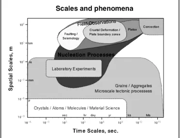
1.3: Geoscience Overview

Earthquake science embodies a richness present in many physical sciences as there are effects present spread over more than ten orders of magnitude in spatial and temporal scales (Figure 1).

4

The microscopic scale (~ 10-6 m to 10-1 m) associated with static and dynamic friction (the primary nonlinearities associ-ated with the earthquake process).

The fault-zone scale (~ 10-1 m to 102 m) that features complex structures containing multiple fractures and crushed rock. The fault-system scale (102 m to 104 m), in which faults are seen to be neither straight nor simply connected, but in which bends, offsetting jogs and sub-parallel strands are common and known to have important mechanical consequences during fault slip.

The regional fault-network scale (104 m to 105 m), where seismicity on an individual fault cannot be understood in isola-tion from the seismicity on the entire regional network of surrounding faults. Here concepts such as "correlaisola-tion length" and "critical state" borrowed from statistical physics have led to new approaches to understanding regional seismicity.

The tectonic plate-boundary scale (105 m to 107 m), at which Planetary Scale boundaries between plates can be approxi-mated as thin shear zones and the motion is uniform at long time scales.

2: GEM COMPUTATIONAL INFRASTRUCTURE (GEMCI)

2.1: Introduction

The components of GEMCI can be divided into eight areas.

1) Overall Framework including agreement to use appropriate “commodity industry standards” such as XML (a language for metadata) and CORBA (a distributed object access standard and broker), as well as more specialized high performance com-puting standards like MPI (Message Passing Interface).

2) Use of GEMCI to construct multiple Problem Solving Environments(PSE’s) to address different scenarios. 3) Web-based User Interface to each PSE

4) Simulation engines built in terms of the GEMCI framework

5) Geophysical-specific libraries such as modules to estimate local physics and friction. These would also use the GEMCI framework which would already include generic libraries

6) Data analysis and Visualization

7) Data Storage, indexing and access for experimental and computational information

8) Complex Systems and Pattern Dynamics Interactive Rapid Prototyping Environment (RPE) for developing new phe-nomenological models -- RPE includes analysis and visualization aspects and would be largely on the client (the local light-weight workstation). In contrast, the large simulations in 4) above, are naturally thought of as distributed server side computa-tional objects.

In the remainder of this Section, we describe the overall GEMCI framework and how it can be constructed in terms of com-ponents built according to emerging distributed object and Web standards and technologies. This describes the “coarse grain” (program level) structure of the GEMCI environment. There are myriad important details inside each module (or grain), which could be a finite element simulation code, data streaming from a sensor, a visualization subsystem, a Java eigensolver used in the client RPE or field data archived in a web-linked database. In Section 3, we describe some of the existing simulation mod-ules available to the GEM collaboration while Section 4 goes into one case in detail. This is the use of fast multipole methods in large-scale Green’s function computations. Section 5 illustrates how these ideas can be integrated together into a variety of different scenarios. These essentially correspond to different problem solving environments that can be built by using the same GEMCI framework to link GEM components in various ways. In Section 6, we make brief remarks on other parts of the GEMCI framework and speculate a little on the future.

There are several important activities which have pioneered the use of object based techniques in computational science. Le-gion has developed a sophisticated object model optimized for computing (http://www.cs.viginia.eu/ ~legion/) and such a framework could be integrated into GEMCI. Currently we are focussing on broad capabilities available in all important dis-tributed object approaches and we can refine this later as we develop more infrastructure. Nile developed the use of CORBA for experimental data analysis (http://www.nile.utexas.edu/) but we need a broader functionality. POOMA is an interesting technology developed at Los Alamos (http://www.acl.lanl.gov/Poo-maFramework/) aimed at object oriented methods for finer grain objects used to build libraries as discussed in Section 2.5. GEMCI could use modules produced by POOMA as part of its repository of coarse grain distributed components.

2.2: Distributed Objects and the Web

5

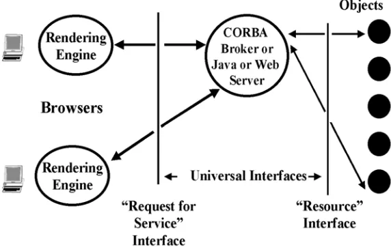
2.2.1: Multi-Tier Architectures. Modern information systems are built with a multi-tier architecture that generalizes the tra-ditional client-server to become a client-broker-service model. This is seen in its simplest realization with the classic web ac-cess which involves 3 tiers – the Browser runs on a client; the middle-tier is a Web server; the final tier or backend is the file system containing the Web page (Figure 2). One could combine the Web server and file system into a single entity and return to the client-server model. However the 3-tier view is better as it also captures the increasingly common cases where the Web Server does not access a file system but rather the Web Page is generated dynamically from a backend database or from a computer program invoked by a CGI script. More generally the middle tier can act as an intermediary or broker that allows many clients to share and choose between many different backend resources. This is illustrated in Figure 3, which shows this architecture with the two interfaces separating the layers. As we will discuss later the specific needs and resources of the Earthquake community will be expressed by metadata at these interfaces using the new XML technology.

This 3-tier architecture (often generalized to a multi-tier system with several server layers) captures several information sys-tems which generalize both the web-page access model of Figure 2 and the remote computer program invocation model of Figure 4.

The architecture builds on modern distributed object technology and this approach underlies the “Object Web” approach to building distributed systems. Before describing this, let us define and discuss several computing concepts.

2.2.2: Clients, Servers and Objects. A server is a free standing computer program that is typically multi-user and in its most simplistic definition, accepts one or more inputs and produces one or more outputs. This capability could be implemented completely by software on the server machine or require access to one or more (super)computers, databases or other informa-tion resources such as (seismic) instruments.

A client is typically single-user and provides the interface for user input and output. In a distributed system, multiple servers and clients, which are in general geographically distributed, are linked together. The clients and servers communicate with messages for which there are several different standard formats.

An (electronic) object is essentially any artifact in our computer system. Two examples among many are displayed in Figure 4. One kind is simply a computer program. The best-known distributed object is a web page.

In the example of Figure 2, a Web Server accepts an HTTP request and returns a web page. HTTP is a simple but universal protocol (i.e. format for control information) for messages specifying how Web Clients can access a particular distributed ob-ject – the web page. A Database Server accepts an SQL request and returns records selected from the database. SQL defines a particular “Request for Service” in the interface of Figure 3 but usually the messages containing these requests use a proprie-tary format. New standards such as JDBC (The Java Database Connectivity) imply a universal message format for database access with vendor dependent bridges converting between universal and proprietary formats. An Object Broker as in Figure 4 uses the industry CORBA standard IIOP message protocol to control the invocation of methods of a distributed object (e.g. run a program). IIOP and HTTP are two standard but different protocols for communicating between distributed objects.

2.2.3: Services in a Distributed System. Distributed objects are the units of information in our architecture and we need to provide certain critical operating system services to support them. Services include general capabilities such as “persistence” (store information unit as a disk file, in a database or otherwise), and “security” as well as more specialized capabilities for sci-ence such as visualization. One critical set of services is associated with the unique labeling of objects and their look-up. We are familiar with this with Domain Name Servers and Yellow Page services for computers on the Internet. Web pages with URL’s build on this technology and Web search engines like Alta Vista provide a sophisticated look-up service. More general objects can use natural variants of this approach with a possibly arcane URL linking to a database, supercomputer or similar resource. The “resource” interface in Figure 3 defines the properties of back-end resources and how to access them. In particu-lar it defines the equivalent of a URL for each object. The set of these resource specifications forms a database, which defines a distributed object repository.

2.2.4: XML Extended Markup Language. The new XML technology is used to specify all resources in the GEMCI. A good overview of the use and importance of XML in Science can be found in Bosak and Bray (1999, http://www.sciam.com/1999/0599issue/0599bosak.html) and we illustrate it in Figure 5, which specifies a computer program used in a prototype GEM problem solving environment described later and shown in Figure 15.

6

information, which is expressed as a stream of objects. These objects need to be “serialized” so as to be transportable between servers. There are many ways of converting complex data-structures into a stream of bytes but XML is one of the most general and often the best choice.

2.2.5: Dynamic Resources. Traditionally one labels a computer with an IP address that reflects a particular physical domain, or addresses a web page with a URL, which reflects a particular server and file system. This approach is appropriate for a fixed resource but not well designed for mobile or dynamic resources such as palm top devices and the growing number of Internet enabled consumer products. These resources are often transient and one cannot assume their continuous availability. There is substantial academic and commercial interest in new object registration, look-up and connection approaches supporting fault tolerance and dynamic clients and servers. Objects must be self defining and able to announce themselves universally to a net-work of registration servers. Jini from Sun Microsystems (http://www.sun.com/jini/) and the Ninja system from UC Berkeley (http://ninja.cs.berkeley.edu/) are well known examples of new approaches to dynamic objects. This technique can be used for both programs and data sets as objects. Thereby either new compute capabilities or new information (raw from sensors or processed) can be dynamically incorporated into simulation systems.

2.2.6: The Object Web. The Object Web signifies the merger of distributed object and web technologies, which is implicitly embodied in the discussion above. There are four rather distinct but important object standards.

CORBA is the Industry Standard supporting objects in any language on any platform. New features in CORBA tend to be deployed relatively slowly as they have a cumbersome approval process and must satisfy complex constraints.

COM is the Microsoft standard, which is confined to PC’s but broadly deployed there and high performance.

Java is the software infrastructure of the web and although single language, the same object can be used on any computer supporting the Java VM.

XML comes from the Web Consortium and has been briefly described above. It can be used to define general objects in an intuitive format illustrated in Figure 5.

The Pragmatic Object Web implies that there is no outright winner in the distributed object field and one should mix and match approaches as needed. For instance, CORBA Objects can use interfaces (as in Figure 3) defined in XML, Clients and Servers programmed in Java, with rendered displays using COM.

2.3: Architecture of the GEMCI Problem Solving Environment

A Problem Solving Environment or PSE is an application that integrates access to the data, computers and tools needed for a particular computational science area. There is general agreement that Object Web technology is the natural software infra-structure for building PSE’s, for the entities one needs to integrate can be considered as distributed objects. With this choice, there is a growing trend to term web-based PSE’s as portals in analogy to the term used to describe environments built com-mercially to allow access to personal or business information. Commercial portals allow both administrative and user custom-izability from a suite of objects and services supporting them.

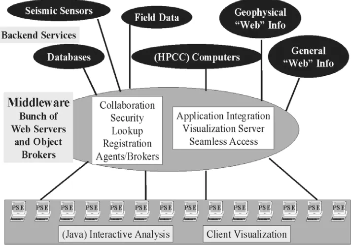
GEMCI illustrated in Figure 6, is an Object Web PSE and has the classic three-tier structure discussed above.

In GEMCI, everything is a “distributed object” whether it be a simulation on a supercomputer, the basic GEM Web pages, the notes from a field trip entered on a palm top, CNN real-time coverage of the latest earthquake or the data streaming in from sensors. GEMCI provides an integrated view of these diverse resources with XML definitions for the raw objects themselves and the data they produce. The services shown in Figure 6, from collaboration, security, object discovery, visualization and computer access, are generic to all computing portals. Building GEMCI using the same approach and tools as other portals en-sures the availability of these services. They will require customization as for instance there are many different visualization packages and each requires non-trivial work to include in such a portal. Again, collaboration corresponds to sharing distributed objects, and this can currently only be automated for some objects. Many web pages can be shared using generic techniques illustrated in Figure 5 but sharing say the control and output of a general simulation can require quite a lot of custom modifica-tions.

Most importantly, to use GEMCI shown in Figure 6, one needs to define the entities in the GEM environment as distributed objects. For computer programs this implies a rather arcane process termed “wrapping the program as a distributed object”. Operationally this implies allowing a middle-tier server (the CORBA object broker or Java application Server) to be able to run the program on one or more machines, specify the input files and either specify output files or access them as streams of data in the fashion of UNIX pipes. Each distributed object technology has a rather different approach to this using what is termed an IDL or Interface Definition Language and specialized Java and C++ code to implement the wrapping.

7

– COM CORBA, and Java – by changing the filter. In this way one can adapt to changes in the commercial infrastructure used in the middle tier.

One must apply the XML object definition strategy to all entities in GEMCI; programs, instruments and other data sources and repositories. This gives the metadata defining macroscopically the object structure. In addition, one needs to look at the data stored in, produced by or exchanged between these objects. This data is itself a typically a stream of objects, each an ar-ray, a table or more complex data structure. One could choose to treat the data at some level as an unspecified (binary) “blob” with XML defining the overall structure but detailed input and output filters used for the data blobs. As an example, consider the approach that an electronic news organization could take for their data. The text of news flashes would be defined in XML but the high volume multimedia data (JPEG images and MPEG movies) would be stored in binary fashion with XML used to specify <IMAGEOBJECT> or <MOVIEOBJECT> metadata.

As explained earlier, systematic use of XML allows use of a growing number of tools to search for, manipulate, persistently store and render the information. It facilitates the linkage of general and specific tools/data sources/programs with clearly de-fined interfaces. This will help the distributed GEM collaborators to separately develop programs or generate data, which will be easily able to interoperate.

More generally XML standards will be defined hierarchically starting with distributed information systems, then general sci-entific computing and finally application specific object specifications.

For example GEMCI would develop its own syntax for seismic data sensors but could build on general frameworks like the XSIL scientific data framework developed by Roy Williams at Caltech (http://www.cacr.caltech.edu/SDA/x-sil/index.html). XSIL supports natural scientific data structures like arrays and the necessary multi-level storage specification.

Another example is MathML which provides XML support for the display and formulation of Mathematics. We can expect MathML to be supported by tools like Web Browsers and white boards in collaborative scientific notebooks and allow one to enhance theoretical collaboration in GEM. There will for instance be modules that can be inserted into applications for parsing MathML or providing graphical user specification of mathematical formulae. This could be used in sophisticated implementa-tions of the Complex Systems and Pattern Dynamics Interactive Rapid Prototyping Environment with scripted client side specification of new analysis methods. One can also use MathML in high level tools allowing specification of basic differential equations that are translated into numerical code. This has been demonstrated in prototype problem solving environments like PDELab but have so far not had much practical application (Houstis et al., 1998 and http://www.cs.pur-due.edu/research/cse/pdelab/pdelab.html). Greater availability of standards like MathML should eventually allow more power-ful interchangeable tools of this type.

Finally we can mention a set of graphical XML standards such as X3D (3 dimensional objects) and VML which is a vector graphics standard, which can be expected to be important as basis of application specific plot and drawing systems.

2.4: Building the GEMCI Problem Solving Environment

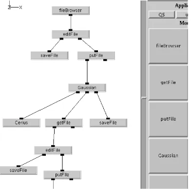
We have described above some aspects of the base strategy of defining GEM components as distributed objects. Here we discuss some existing experience from NPAC at Syracuse in integrating such objects and tools that manipulate them into an overall environment. The NPAC team has built several exemplar problem solving environments for both the NSF and DoD HPCMO (High Performance Computing Modernization Office) supercomputer centers. In Figure 7, we show some useful tools including a first cut at a “wizard” that helps produce the distributed object wrappers described above.

This AAD (Abstract Application Descriptor) can be extended to allow specification of all needed input parameters of an ap-plication, with an automatic generation of input forms respecting default values and allowed value ranges. The object wrappers of an application should not only invoke the code and allow parameter specification but have built in description/help systems.

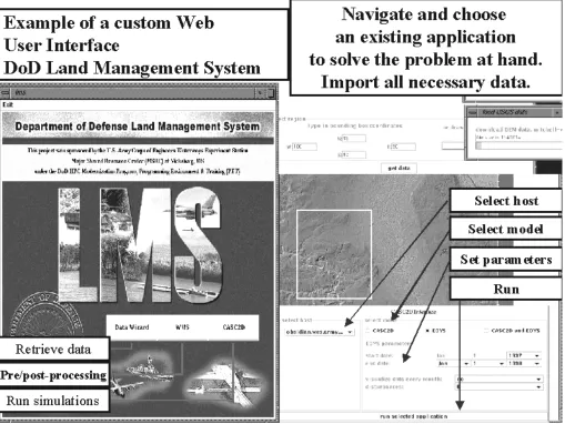
One major NPAC Problem Solving Environment was built for the Landscape Management System (LMS) project at the U.S. Army Corps of Engineers Waterways Experiment Station (ERDC) Major Shared Resource Center (MSRC) at Vicksburg, MS, under the DoD HPC Modernization Program, Programming Environment and Training (PET). The application can be idealized as follows.

A decision maker (the end user of the system) wants to evaluate changes in vegetation in some geographical region over a long time period caused by some short term disturbances such as a fire or human activities. One of the critical parameters of the vegetation model is soil condition at the time of the disturbance. This in turn is dominated by rainfall that possibly occurs at that time. Consequently as shown in Figure 8, the implementation of this project requires:

1) Data retrieval from remote sources including DEM (data elevation models) data, land use maps, soil textures, dominating flora species, and their growing characteristics, to name a few. The data are available from many different sources, for example from public services such as USGS web servers, or from proprietary databases. The data come in different formats, and with different spatial resolutions.

8

3) Execution of two simulation programs: EDYS for vegetation simulation including the disturbances and CASC2D for wa-tershed simulations during rainfalls. The latter results in generating maps of the soil condition after the rainfall. The initial conditions for CASC2D are set by EDYS just before the rainfall event, and the output of CASC2D after the event is used to update parameters of EDYS and the data transfer between the two codes had to be performed several times during one simula-tion. EDYS is not CPU demanding, and it is implemented only for Windows95/98/NT systems. On the other hand, CASC2D is very computationally intensive and typically is run on powerful backend supercomputer systems.

4) Visualization of the results of the simulation. Again, WMS is used for this purpose.

One requirement of this project was to demonstrate the feasibility of implementing a system that would allow launching and controlling the complete simulation from a networked laptop. We successfully implemented it using WebFlow middle-tier servers with WMS and EDYS encapsulated as WebFlow modules running locally on the laptop and CASC2D executed by WebFlow on remote hosts. Further the applications involved showed a typical mix of supercomputer and computationally less demanding personal computer codes. LMS was originally built using specialized Java Servers but these are now being re-placed by commercial CORBA object brokers but in either case the architecture of Figure 8 is consistent with the general structure of Figures 6 and 3.

For this project we developed a custom front-end shown in Figure 9, that allows the user to interactively select the region of interest by drawing a rectangle on a map. Then one could select the data type to be retrieved, launch WMS to preprocess the data and make visualizations, and finally launch the simulation with CASC2D running on a host of choice.

Our use of XML standards at the two interfaces in Figure 3, allows us to change front end and middle-tier independently. This allowed us the middle tier upgrade described above which will bring security and “seamless access” capability to our PSE’s.

Seamless access is an important service, which is aimed at allowing applications to be run on an arbitrary appropriate backend. Most users wish their job to just run and usually do not mind what machine is used. Such seamless capability is rather natural in the architecture of Figure 3. Essentially the front end defines the “abstract” job passing its XML specification to a middle tier server. This acts as a broker and instantiates the abstract job on one of the available backend computers. The middle-tier backend XML interface is used to specify both the available machines sent to the servers and the “instantiated job” sent from the servers. We build the back end mapping of jobs to machine using the important Globus technology (http://www.glo-bus.org). Globus is a distributed or meta-computing toolkit providing important services such as resource look-up, security, message passing etc.

One can view WebFlow (Figures 7 and 8) as a “kit” of services, which can be used in different ways in different applica-tions. In Figure 10, we show another capability of WebFlow, which supports the ability to compose complex problems by link-ing different applications together with data flowlink-ing between different modules chosen from a palette. This WebFlow service is supported by a Java front end and a middle tier service matching abstract modules to back end computers and supporting the piping of data between the modules.

2.5: Libraries or Distributed Components?

Since the beginning of (computing) time, large programs have been built from components that are assembled together into a complete job. One can do this in many ways and perhaps the best known is the use of libraries linked together. Modern “ob-ject-oriented” approaches can be used in this fashion with method calls. Design frameworks can be used to establish a system-atic methodology with say specific interfaces (“calling sequences”) to be followed by for instance different implementations of friction laws. The discussion in Section 2.4 above describes a rather different component model where possibly distributed modules are linked together in a dynamic fashion. This is more flexible than the library approach and further as explained above, this supports distributed components. The component approach is not surprisingly less efficient than the library ap-proach as component linkage is typically obtained through explicit exchange of messages rather than efficient compiled gener-ated parameter passing as for library methods. The inefficiency is particularly serious for small components as the component mechanisms come with large start up (latency) overheads. Thus we adopt a hybrid approach with small objects using the tradi-tional library mechanism within a set of agreed interfaces and design frameworks to promote easier interchange of modules. On the other hand, large objects (roughly “complete programs”) use a component approach within a distributed object frame-work, which is defined in XML.

3: CURRENT GEM COMPUTATIONAL COMPONENTS

9

The categories covered by the existing codes include codes for understanding dislocations: elastic models - both half-space and layered, viscoelastic models, finite element and boundary element codes, and inversion codes. There are a set of codes for understanding how faults interact: cellular automata, finite element and boundary element codes, fault friction models. Some codes are designed to understand the dynamics of the earthquake rupture itself. Finally there are codes for displaying the re-sults of various simulations. We follow with short descriptions of the codes grouped by type.

Elastic

3D-DEF -- Performs elastic dislocation boundary-element calculations

coulomb -- Computes 3D elastic dislocation & 2D boundary element stress and strain DYNELF -- Models 3D elastodynamic finite difference with frictional faults

faultpatch -- Generates earthquake sequences, given fault geometries and loading rates using

FLTSLP -- Inverts groups of focal mechanism solutions or slickenline data for orientation and relative magnitudes of prin-cipal strain rates and for relative micropolar vorticity.

GNStress -- Model stresses induced by faulting, for studying fault interaction.

layer -- Calculates surface displacements and strains for vertical strike-slip point source in horizontal layer above half-space. RNGCHN -- Calculate surface displacements and strains in elastic half space.

scoot -- 2D elastodynamic finite difference with frictional fault simplex -- 3D inversion of geodetic data for displacement on faults.

Viscoelastic

DYNELF -- Models 3D elastodynamic finite difference with frictional faults

FLTGRV and FLTGRH -- Compute 3 vector components of surface displacement from slip on a dipping thrust fault con-tained within an elastic layer overlying a viscoelastic-gravitational half space.

STRGRH and STRGRV -- Computes 3 vector components of surface displacement from slip on a dipping strike slip fault contained within an elastic layer overlying a viscoelastic-gravitational half space.

Virtual_California -- Realistic cellular automata (CA) viscoelastic earthquake simulator. VISCO1D -- Computes viscoelastic spherical deformation due to faulting or dike emplacement.

Cellular Automata

faultpatch -- Generates earthquake sequences, given fault geometry’s and loading rates using Cellular automata methods. Virtual_California -- Realistic cellular automata (CA) viscoelastic earthquake simulator.

Dynamic

DYNELF -- Models 3D elastodynamic finite difference with frictional faults scoot -- 2D elastodynamic finite difference with frictional fault

Inverse

FLTSLP -- Inverts groups of focal mechanism solutions or slickenline data for orientation and relative magnitudes of prin-cipal strain rates and for relative micropolar vorticity.

simplex -- 3D inversion of geodetic data for displacement on faults.

qoca – optimal combining of various geodetic measurments resulting in a consistent deformation field.

Visualization

10

4: LARGE-SCALE SIMULATIONS IN GEMCI

4.1: Overview of Earthquake Fault System Simulations

With reasonable approximation, one may model the long-term evolution of stresses and strains on interacting fault segments with a Green's function approach. As in other fields this method leads to a boundary (the faults) value formulation, which looks numerically, like the long-range force problem. The faults are paneled with segments (with area of some 100 m2 _in

de-finitive computations) which interact as though they were dipoles. The original calculations of this model used the basic O(N2₎

algorithm but a new set of codes will be using the "fast multipole" method adapted from gravitational-particle astrophysics. There are interesting differences between the earthquake and gravitational applications. In gravity we get wide ranges in den-sity and dynamical effects from the natural clustering of the gravitating particles. Earthquake "particles" are essentially fixed on complex fault geometries and their interactions fall off faster than those in the astrophysical problem.

Several variants of this model have been explored including approximations, which only keep interactions between nearby fault segments. These "cellular automata" or "slider-block" models look very like statistical physics with an earthquake corre-sponding to clusters of particles slipping together when the correlation length gets long near a critical point. The full Green's function approach should parallelize straightforwardly in either O(N2_{) or multipole formulation. However cellular automata}

models will be harder to parallelize, as we know from experience with the corresponding statistical physics case where cluster-ing models have been extensively studied.

An interesting aspect of these simulations is that they give the "numerical laboratory" for the study of space-time patterns in seismicity information. This type of analysis was used successfully in the climate field to aid the prediction of "El Nino" phe-nomena. These pattern analyses may or may not need large computational resources although they can involve determination of eigensolutions of large matrices which is potentially time consuming.

4.2: Green’s Function Formulation and Approximations

4.2.1: Basic Equations. Let us consider in more detail the problem addressed by the Virtual_California code described in Section 3 and introduced in Rundle 1988a. If one is given a network of faults embedded in an Earth with a given rheology, subject to loading by distant stresses, and neglecting elastic waves (see discussion below), the evolution of the state of slip s(x, t) on a fault at (x, t) is determined from the equilibrium of stresses according to Newton's Laws:

∂s(x, t) / ∂t = Φ{

Σ

where Φ{} is a nonlinear functional, and

Σ

in-clude

1) The interaction stress σint[x,t; s(x',t'); p] provided by transmission of stress through the Earth's crust arising from

back-ground tractions p, as well as stresses due to slip on other faults at other sites x' at times t';

2) The cohesive fault frictional stress σf[x,t; s(x,t)] at the site (x,t) associated with the state of slip s(x,t); and

3) Other stresses such as those due to dynamic stress transmission and inertia.

The transmission of stress through the Earth's crust involves both dynamic effects arising from the transient propagation of seismic waves, and from static effects that persist after wave motion has ceased. Rheologic models typically used for the Earth's crust between faults are all linear (e.g., Rundle and Turcotte, 1993) and include

1) A purely elastic material on both long and short time scales;

2) A material whose instantaneous response is elastic but whose long term deformation involves bulk flow (viscoelastic); and

3) A material that is again elastic over short times, but whose long term response involves stress changes due to the flow of pore fluids through the rock matrix (poroelastic).

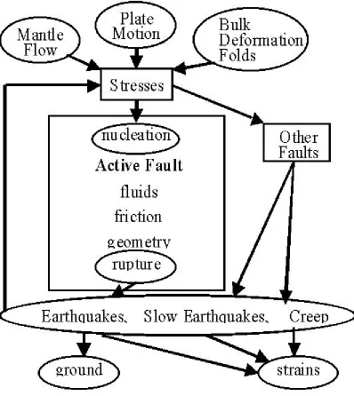
In Figure 11, we show the basic conceptual "wiring diagram" for the model, which indicates the interplay between loading stresses, rupture, interactions with other faults, and relaxation processes following a major earthquake.

4.2.2: The Green's Function Approximation. Considering GEM models that assume a linear interaction rheology between the faults implies that the interaction stress can be expressed as a spatial and temporal convolution of a stress Green's function Tijkl(x – x', t – t') with the slip deficit variable φ(x, t) = s(x, t) – Vt, where V is the long term rate of offset on the fault. Once

the slip deficit is known, the displacement Green's function Gijk(x – x', t – t') can be used to compute, again by convolution, the

11

evidence supports the hypothesis that simulations carried out without including inertia and waves will have substantial physi-cal meaning. Kanamori and Anderson (1975) estimated that the seismic efficiency η, which measures the fraction of energy in the earthquake lost to seismic radiation, is less than 5%-10%. This implies that inertial effects in the dynamical evolution of slip in studying large populations of earthquakes will be of lesser importance for initial calculations. Elastic waves will be in-cluded in later simulations when errors arising from other effects are reduced to the 5%-10% level. At present, inclusion of these effects is severely limited by available computational capability, so we anticipate that it may be practical to include only the longest wavelengths or largest spatial scales.

4.2.3: Inelastic Rheologies. In quasistatic interactions, the time dependence of the Green's function typically enters only im-plicitly through time dependence of the elastic moduli (e.g., Lee, 1955). Because of linearity, the fundamental problem is re-duced to that of calculating the stress and deformation Green's function for the rheology of interest. For materials that are ho-mogenous within horizontal layers, numerical methods to compute these Green's functions are well known (e.g., Okada, 1985, 1992; Rundle, 1982a,b, 1988; Rice and Cleary, 1976; Cleary, 1977; Burridge and Varga, 1979; Maruyama, 1994). Problems in heterogeneous media, especially media with a distribution of cracks too small and too numerous to model individually, are often solved by using effective medium approaches, self-consistency assumptions (Hill, 1965; Berryman and Milton, 1985; Ivins, 1995a,b), or damage models Lyakovsky et al. (1997). Suffice to say that a considerable amount of effort has gone into constructing quasistatic Green's functions for these types of media, and while the computational problems present certain chal-lenges, the methods are straightforward as long as the problems are linear. In the initial work, we expect to focus on elastic (with possible incorporation of damage parameters) and layered viscoelastic models only.

4.3: Friction Models:

Friction models to determine the slip condition must augment the overall differential equations. At the present time, six basic classes of friction laws have been incorporated into computational models. They fall into three families as follows.

1)Two basic classes of friction models arise from laboratory experiments:

Slip Weakening. This friction law (Rabinowicz, 1965; Bowdon and Tabor, 1950; Beeler et al., 1996; Li, 1987; Rice, 1993; Stuart and Tullis, 1995) assumes that the frictional stress at a site on the fault σ_f = σ_f[s(x, t)] is a functional of the state of slip. In general, σ_f[s(x, t)] is peaked at regular intervals. The current state of the system is found from enforcing the equality

σf[s(x, t)] = σint[x, t; s(x', t'); p] prior to, and just after, a sliding event.

Rate and State. These friction laws are based on laboratory sliding experiments in which two frictional surfaces are slid over each other at varying velocities, usually without experiencing arrest (Dieterich, 1972; 1978; 1981; Ruina, 1983; Rice and Ruina, 1983; Ben Zion and Rice, 1993; 1995; 1997; Rice, 1993; Rice and Ben Zion, 1996). In these experiments, the labora-tory apparatus is arranged so as to be much “stiffer” than the experimental “fault” surfaces. The rate dependence of these fric-tion laws refers to a dependence on logarithm of sliding velocity, and the state dependence to one or more state variables θ_i(t), each of which follows an independent relaxation equation.

2)Two classes of models have been developed and used that are based on laboratory observations, but are computationally simpler.

Coulomb-Automata. These are widely used because they are so simple (e.g., Rundle and Jackson, 1977; Nakanishi, 1991; Brown et al., 1991; Rundle and Brown, 1991; Rundle and Klein, 1992; Ben Zion and Rice, 1993, 1995, 1997). A static failure threshold, or equivalently a coefficient of static friction µS _{is prescribed, along with a residual strength, or equivalently a}

dy-namic coefficient of friction µD_{. When the stress at a site increases, either gradually or suddenly, to equal or exceed the static}

value, a sudden jump in slip (change of state) occurs, that takes the local stress down to the residual value. These models natu-rally lend themselves to a Cellular Automaton (CA) method of implementation.

Velocity Weakening. This model (Burridge and Knopoff, 1967; Carlson and Langer, 1989) is based on the observation that frictional strength diminishes as sliding proceeds. A constant static strength σf = σF is used as above, after which the

assump-tion is made that during sliding, fricassump-tional resistance must be inversely proporassump-tional to sliding velocity.

3) Two classes of models are based on the use of statistical mechanics involving the physical variables that characterize stress accumulation and failure. Their basic goal is to construct a series of nonlinear stochastic equations whose solutions can be approached by numerical means:

Traveling Density Wave. These models (Rundle et al., 1996) are based on the slip weakening model. The principle of evo-lution towards maximum stability is used to obtain a kinetic equation in which the rate of change of slip depends on the func-tional derivative of a Lyapunov funcfunc-tional potential. This model can be expected only to apply in the mean field regime of long range interactions, which is the regime of interest for elasticity in the Earth. Other models in this class include those of Fisher et al. (1997) and Dahmen et al. (1997).

12

models in which hierarchies of blocks or asperity sites are assigned probabilities of failure. As the level of external stress rises, probabilities of failure increase, and as a site fails, it influences the probability of failure of nearby sites.

4.4: Multipole Methods and Fast Numerical Simulation

4.4.1: Introduction. The GEM group has started to investigate the use of advanced parallel solvers for the codes described in Section 3. The Green’s function approach can be formulated numerically as a long-range all-pairs interaction problem and this can be straightforwardly parallelized using well-known algorithms. However one cannot reach the required level of resolution without switching from an order O(N2) to one of the O(N) or O(N logN) approaches. As in other fields, this can be achieved by dropping or approximating the long-range components and implementing a neighbor-list based algorithm. However it is more attractive to formulate the problem as interacting dipoles and adapt existing fast-multipole technology developed for particle dynamics problems. We have already produced a prototype general purpose “fast multipole template code” by adapting the very successful work of Salmon and Warren (1997). These codes have already simulated over 300 million gravitating bodies on a large distributed memory system (a 4500-processor subset of the ASCI “Red” machine), so we expect these parallel algo-rithms to scale efficiently up to the problem sizes needed by GEM.

4.4.2: Multipolar Representation of Fault Systems. A primary key to a successful implementation of GEM models of faults systems will be to utilize computationally efficient algorithms for updating the interactions between fault segments. Convert-ing the Green's function integrals to sums, without truncation or approximation, would require O(N2) operations between earthquakes, and possibly more for segments of faults experiencing an earthquake. For quasistatic interactions, the Green's functions Tijkl and Gijk for linear elasticity have a simple time dependence. Moreover, the Green's functions for linear

viscoe-lasticity and for linear poroeviscoe-lasticity can be obtained from the elastic Green's functions using the correspondence principle (e.g., Lee, 1955; Rundle 1982a,b). These simplifications strongly suggest that multipole expansions (Goil, 1994; Goil and Ranka, 1995) will be computationally efficient algorithms.

The stress and displacement Green's functions Tijkl and Gijk represent the tensor stress and vector displacement at x due to a

point double couple located at x' (Steketee, 1958). The orientation at x' of the equivalent fault surface normal vector, and of the vector displacement on that fault surface, are described by the indices i and j. Displacement and stress indices at the field point x are described by indices k and l. Integration of Tijkl and Gijk over the fault surface then corresponds to a distribution of

dou-ble couples. For that reason, representation of the stress over segments of fault in terms of a multipole expansion is the natural basis to use for the GEM computational problem. In fact, the use of multipolar expansions to represent source fields in earth-quake and explosion seismology was introduced by Archambeau (1968) and Archambeau and Minster (1978), and later revis-ited from a different perspective by Backus and Mulcahy (1976). Minster (1985) gives a review of these early representations. 4.4.3:Application of Fast Multipole Methods to GEM. In the gravitational N-body problem, each body interacts with every other one in the system according to the familiar law of gravitational attraction. Simply computing all pairs of interactions re-quires N(N-1)/2 separate evaluations of the interaction law. This formulation of the problem has some important advantages: it is easy to code, it is easy to vectorize and parallelize, it is readily expressible in High Performance Fortran, and it is even ame-nable to special-purpose hardware [e.g. GRAPE]. Nevertheless, even today's fastest special-purpose systems, running in a dedicated mode for extended times at rates of nearly 1 TERAFLOP, cannot simulate systems larger than about 100,000 bodies. Tremendous computational savings may be realized by combining bodies into “cells” and approximating their external field with a truncated multipole expansion. When this idea is applied systematically, the number of interactions may be reduced to O(N logN) (Appel, 1985; Barnes and Hut, 1986) or O(N) (Greengard and Rokhlin, 1987; Anderson, 1992). The cells are gen-erally arranged in a tree, with the root of the tree representing the entire system, and descendants representing successively smaller regions of space. Salmon and Warren (1997) have demonstrated that such codes can run in parallel on thousands of processors and have simulated highly irregular cosmological systems of over 300 million bodies using ASCI facilities.

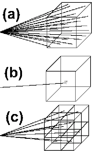
The basic idea of fast multipole methods is shown in the three versions of Figure 12. In 12(a), we show the simple O(N2₎

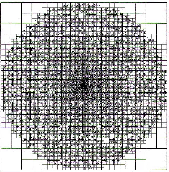
ap-proach with a single particle on the left interacting with all the individual particles in a box on the right. The naïve computa-tional simplification shown in Figure 12(b) is to replace (in the gravity case) the particles by their center of mass and use a sin-gle force calculation. However this approximation may not be accurate enough and so in Figure 12(c) we show the original box broken into 8 sub-boxes with the total summed over the individual sub-box contributions. This idea can be automated and implemented in a clever way so that the boxes used get smaller as you move closer to a given particle or if there is significant variation in particle density. Further there are subtle but very efficient parallel versions of the method to build the set of hierar-chical sub-boxes (which form a tree so that these are often termed tree codes) which in the case of gravity is rebuilt each time step. In Figure 13 below, we illustrate the adaptive division generated for 10,000 particles clustered in a two-dimensional disk.

13

sources in a region by a multipole expansion, the external field generated by a large number of bodies can be computed to any desired degree of accuracy in constant time. Thus, the GEM problem can also be reduced to O(NlogN) or O(N) total interac-tions, so that large calculations are tractable. On the other hand, although multipole methods can deliver large performance gains, they also require a considerable infrastructure. This is especially true of efficient parallel implementations. We intend to develop the multipole version of GEM using a library that has been abstracted from Salmon and Warren's successful astro-physical N-body codes. This new library is:

Modular - The “physics” is cleanly separated from the “computer science”, so that in principle, alternative physics modules such as the evaluation of the GEM Green's functions, can simply be “plugged in”. The first non-gravitational demonstration was a vortex dynamics code written by Winckelmans et al. (1995).The interface to the physics modules is extremely flexible. A general decision-making function tells the treecode whether or not a multipole, or any other approximation, is adequate for a given field evaluation. Short-range interactions, which vanish outside a given radius, can be handled as well.

Tunable - Careful attention to analytical error bounds has led to significant speed-ups of the astrophysical codes, while re-taining the same level of accuracy. Analytic error bounds may be characterized as quantifying the fact that the multipole for-malism is more accurate when the interaction is weak: when the analytic form of the fundamental interaction is well-approximated by its lower derivatives; when the sources are distributed over a small region; when the field is evaluated near the center of a “local expansion"; when more terms in the multipole expansion are used, and when the truncated multipole moments are small. These issues are primarily the concern of the “physics” modules, but the library provides a sufficiently powerful interface to make these parameters adjustable. The formulation is general enough that the same library can be used to support evaluation of O(N), O(NlogN) and O(N2) approximation strategies, simply by changing the decision criteria and inter-action functions.

Adaptive - The tree automatically adapts to local variations in the density of sources. This can be important for GEM as it is expected that large earthquakes are the result of phenomena occurring over a wide range of length and time scales.

Scalable - The library has been successfully used on thousands of processors, and has sustained 170 Gflops aggregate per-formance on a distributed system of 4096 200Mhz PentiumPro processors.

Out of core - The library can construct trees, and facilitates use of data sets that do not fit in primary storage. This can allow one to invest hardware resources into processing rather than memory, resulting in more computations at constant resources.

Dynamically load balanced - The tree data structure can be dynamically load-balanced extremely rapidly by sorting bodies and cells according to an easily computed key.

Portable - The library uses a minimal set of MPI primitives and is written entirely in ANSI C. It has been ported to a wide variety of distributed memory systems - both 32-bit and 64-bit. Shared memory systems are, of course, also supported simply by use of an MPI library tuned to the shared memory environment.

Versatile - Early versions of the library have already been applied outside the astrophysics and molecular dynamics area. In particular the Caltech and Los Alamos groups have successfully used it for the vortex method in Computational Fluid Dynam-ics.

14

4.5: Computational Complexity

Current evidence suggests that forecasting earthquakes of magnitude ~6 and greater will depend upon understanding the space-time patterns displayed by smaller events; i.e., the magnitude 3's, 4's and 5's. With at least 40,000 km2 _{of fault area in}

southern California, as many as 108 _{grid sites (10-meter segment size) will be needed to accommodate events down to}

magni-tude 3. Extrapolations based upon existing calculations indicate that using time steps of ~100 seconds implies ~108 _{time steps}

will be required to simulate several earthquake cycles. This leads to the need for teraflop class computers in this as in many physical simulations.

Here we make the conservative assumption that the GEM dipole-dipole Green's function evaluations are ten times as compu-tationally expensive as the Newtonian Green's functions evaluated in Salmon and Warren's code. At this stage, we cannot guess how far the teraflop class of computer will take us and the systems needed to support research, crisis managers or insur-ance companies assessing possible earthquake risk, may require much higher performinsur-ance.

4.6: Integration of Simulation Modules into GEMCI

As we described in Section 2.5, we will adopt a hierarchical model for the simulation components used in GEMCI. The full Greens function programs would be macroscopic distributed objects which can be manipulated by systems like WebFlow and linked with other coarse grain components such as sensor data, other programs such as finite-element solvers and visualization systems. These components are made up of smaller objects used in library fashion. Here we have the friction modules and dif-ferent solver engines such as the conventional O(N2_{) and fast multipole methods with each having sequential and parallel}

ver-sions. The latter would often exist in multiple forms including an openMP version for shared memory and MPI version for dis-tributed memory.

5: TYPICAL COMPUTATIONAL PROBLEMS

Here we give three sample scenarios, which would correspond to distinct problem solving environments built using GEMCI.

5.1: Seismicity Models and Data Assimilation

Our first example of how the GEMCI might be used is drawn from an attempt to create a computer model of the seismicity of California or other seismically active region. Such a model, to the extent that it is realistic, could be quite useful in guiding intuition about the earthquake process, and suggesting new measurements or lines of inquiry.

Making such a model realistic requires many different types of data and there are for instance already substantial archives accumulated by the Southern California Earthquake Center (SCEC), as well as the Seismological Laboratory of the California Institute of Technology, and the Pasadena field office of the United States Geological Survey. The relevant data includes:

1) Broadband seismic data from the TERRASCOPE array. 2) Continuous (SCIGN) and “campaign style” geodetic data.

3) Paleoseismic data collected on the major faults of southern California. 4) Near field strong motion accelerograms of recent earthquakes. 5) Field structural geology of major active faults.

6) Other data including GPS data, leveling data, pore fluid pressure, in situ stress, heat flow, downhole seismic data, multi-channel seismic data, laboratory measurements of mechanical properties of various rocks, 3-D geologic structure, gravity data, magneto-telluric data, hydrology data, and ocean tide data (to constrain coastal uplift).

These will be used, for example, to update the fault geometry models used by GEM, and to update fault slip histories used to validate earthquake models.

A new and extremely promising type of geodetic data is Synthetic Aperture Radar Interferometry (InSAR), which permits “stress analysis of the Earth.” A number of SAR missions are currently acquiring data over southern California, including the C-band (5.8 cm) European ERS 1/2 satellites and the L-band Japanese JERS satellite. These missions have already produced revolutionary images of the complete deformation fields associated with earthquakes in the United States and Japan (e.g., Mas-sonnet et al., 1993). These techniques rely on radar interferograms that represent the deformation field at a pixel resolution of a few tens of meters over areas of tens of thousands of square kilometers, and over time intervals of weeks to years. We are now essentially able to see the complete surface deformation field due to an earthquake, with excellent prospects for similar views of deformation due to interseismic strain-accumulation processes.