XXX-X-XXXX-XXXX-X/XX/$XX.00 ©20XX IEEE
Learning Everywhere: A Taxonomy for the
Integration of Machine Learning and Simulations
Geoffrey Fox Indiana University
Bloomington, IN [email protected]
Shantenu Jha Rutgers University and Brookhaven National Laboratory
Abstract—We present a taxonomy of research on Machine Learning (ML) applied to enhance simulations together with a catalog of some activities. We cover eight patterns for the link of ML to the simulations or systems plus three algorithmic areas: particle dynamics, agent-based models and partial differential equations. The patterns are further divided into three action areas: Improving simulation with Configurations and Integration of Data, Learn Structure, Theory and Model for Simulation, and Learn to make Surrogates.
Keywords—HPC, Machine Learning, Simulation
I.
I
NTRODUCTION [image:1.612.45.296.316.489.2]A.
Introduction
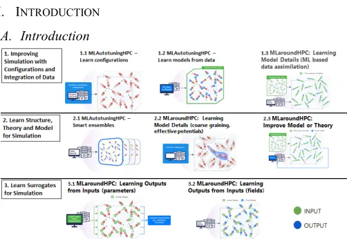
Fig. 1. The 8 MLAutotuning and MLaroundHPC scenarios described in text
This taxonomy of research at the intersection of Machine
Learning and Simulations builds on papers below.
1)
A quadrology of papers on learning everywhere [1]–[4].
The first paper gives an overview and the unpublished
second report adds detail on
Technology, Network
Science, nanoengineering, biomolecular and
computational biology (virtual tissues). The third paper
develops the underpinnings of learning everywhere and the
fourth is this paper. There are also presentations at BDEC
[5]
and at IPDPS
[6]
.
2)
Jeffrey Dean presentation at NeurIPS 2017 on Machine
learning for systems and systems for machine learning [7]
3)
Microsoft 2018 Faculty Summit presentations on AI for
Systems
[8], [9]
4)
Satoshi Matsuoka on the convergence of AI and HPC
[10]
5)
An NSF funded project mainly focused on HPCforML
[11], [12]
We now describe the categories used below to categorize
papers [1-3], [5], [13]
•
HPCforML: Using HPC to execute and enhance ML
performance, or using HPC simulations to train ML
algorithms (theory-guided machine learning), which are
then used to understand experimental data or simulations.
•
MLforHPC: Using ML to enhance HPC applications and
systems
We further subdivide HPCforML as
•
HPCrunsML: Using HPC to execute ML with high
performance
•
SimulationTrainedML: Using HPC simulations to train
ML algorithms, which are then used to understand
experimental data or simulations.
We also subdivide MLforHPC into several categories. First we
identify
•
MLControl: Using simulations (with HPC) in control of
experiments and in objective driven computational
campaigns. Here simulation surrogates of MLaroundHPC
are very valuable to allow real-time predictions. This is
discussed in [3]
Then can divide other aspects by whether they are before -
termed MLAutotuningHPC, during the execution - termed
MLaroundHPC, or after - termed MLafterHPC.
•
MLafterHPC: ML analyzing results of HPC as in
trajectory analysis and structure identification in
biomolecular simulations
The other two terms where we focus in this paper are
•
MLAutotuning: Using ML to configure (autotune) ML or
HPC simulations.
•
MLaroundHPC: Using ML to learn from simulations and
produce learned surrogates for the simulations. The same
ML wrapper can also learn configurations as well as
results. This differs from SimulationTrainedML as the
latter is typically using learned network to predict
observation whereas in MLaroundHPC we are using the
ML to improve the HPC performance.
areas and divide them into three types of actions represented
into the three rows of fig. 1 and sections 2, 3 and 4 of this
detailed taxonomy paper. The three action areas are:
II.
Improving simulation with Configurations and
Integration of Data
II.A.
MLAutotuningHPC – Learn configurations of system
and software for particular hardware and input
parameters
II.B.
MLAutotuningHPC – Learn models from data at start
of simulation
II.C.
MLaroundHPC: Learning model details (ML based
data assimilation) dynamically during simulation.
III.
Learn Structure, Theory and Model for Simulation
III.A.
MLAutotuningHPC – Smart ensembles
III.B.
MLaroundHPC: Learning Model Details (coarse
graining, effective potentials)
III.C.
MLaroundHPC: Learning Model Details - Improving
Model or Theory
IV.
Learn to make Surrogates
Here we use ML (typically neural networks) to learn the
function representing the output of the simulation.
IV.A.
MLaroundHPC: Learning Outputs from Inputs
(parameters)
IV.B.
MLaroundHPC: Learning Outputs from Inputs (fields)
These clean atomic categories can appear differently as they
are applied dynamically or differently in different (space or
time) parts of simulation.
In later sections, ABM stands for Agent-Based Simulations
and Data-driven Approaches to ABM systems. The work is
divided into three broad application areas: Particle dynamics,
ABM and Partial Differential Equation based problems. We list
MLAutotuningHPC and MLaroundHPC references divided by
these 3 application areas and the 8 categories summarized in Fig.
1. In this and following 8 expanded figures we use a prototypical
particle dynamics simulation to represent the ML interaction
with green representing input and blue output of interaction.
II.
T
AXONOMY OFMLA
UTOTUNING ANDML
AROUNDHPC:
I
MPROVINGS
IMULATION WITHC
ONFIGURATIONS ANDI
NTEGRATION OFD
ATAA.
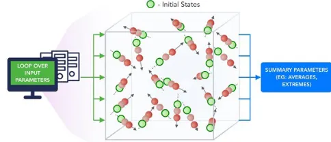
MLAutotuningHPC – Learn configurations
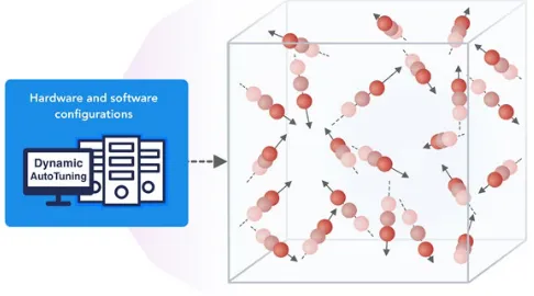
Figure 2 illustrates this category, which is classic Autotuning
and one optimizes some mix of performance and quality of
results with the learning network inputting the configuration
parameters of the computation. The configuration includes
initial values and also dynamic choices such as block sizes for
cache use, variable step sizes in space and time. This category
can also include discrete choices as to the type of solver to be
used.
1)
Particle Dynamics-MLAutotuningHPC – Learn
configurations
1.
Nanoparticle simulations using
ML
to improve
performance
[14]
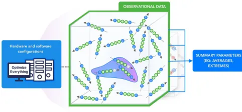
B.
MLAutoTuningHPC: Learning Model Setups from
[image:2.612.316.559.99.234.2]Observational Data
[image:2.612.320.559.288.414.2]Fig. 2. MLAutotuningHPC – Learn configurations
Fig. 3. MLAutoTuningHPC: Learning Model Setups from Observational Data
This category is seen when a simulation set up as a set of
agents, perhaps each representing a cell in a virtual tissue
simulation. Tuning agent (model) parameters to optimize agent
outputs to available empirical data presents one of the greatest
challenges in model construction. As well as directly setting cell
parameters, one can use ML to learn the dynamics of cells
replacing detailed computations by ML surrogates. As there can
be millions to billions of such agents the performance gain can
be huge as each agent uses the same learned model. In this case
one is using MLaroundHPC: Learning Outputs from Inputs for
cells or alternately MLAutotuning for multi-cell (tissue) built
from the cells.
1)
Particle Dynamics-MLAutotuningHPC – Learning
Model Setups from Observational Data
2.
Use of ANN’s to represent dynamics of robots [15]
2)
ABM-MLAutotuningHPC – Learning Model Setups
from Observational Data
4.
Using machine learning (modest emphasis) to represent
cell (agent) behavior based on data for prediction of
cancer cell behavior [17]
5.
Automatic inference of a model of the escape response
behavior in a roundworm directly from time series data
[18] building on [19], [20]. The unknown parameters in a
set of ODE’s are determined by fitting data in a
hierarchical fashion
3)
PDE-MLAutotuningHPC – Learning Model Setups from
Observational Data
6.
Use ANN’s to discover the PDE form of biological
transport equations from noisy data. [21]
C.
MLaroundHPC: Learning Model Details - ML for Data
[image:3.612.48.288.249.403.2]Assimilation (predictor-corrector approach)
Fig. 4. MLaroundHPC: Learning Model Details - ML for Data Assimilation (predictor-corrector approach)
Data assimilation involves continuous integration of time
dependent simulations with observations to correct the model
with a suitable combined data plus simulation model. This is for
example common practice in weather prediction field. We see
this approach becoming even more important with new machine
learning approaches now available and under intense research
for many time series based problems such as work on ride
hailing [22]. Such current state of the art expresses the spatial
structure as a convolutional neural net and the time dependence
as recurrent neural net (LSTM). We expect this category to grow
in importance and interest. This category extends the previous
one in sec. 2.1.2 with dynamic interplay between model and
data.
Often the data consists of “videos” recording observational
data, which is a high dimensional (spatial extent) time series.
Then as a function of time one iterates a predictor corrector
approach, where one time steps models and at each step optimize
the parameters to minimize divergence between simulation and
ground truth data. As an example considered by a team led by
Glazier at Indiana University, one produces a generic
agent-based model organism such as an embryo. Then one could take
this generic model as a template and learn the different
adjustments for particular individual organisms.
1)
ABM-MLaroundHPC: Learning Model Details (ML
based data assimilation)
7.
Using data to predict solutions of complex coupled
Agents for metabolic pathway dynamics [23]
8.
Deep Learning RNN and CNN to predict epidemics
viewed as time series [24]
9.
LSTM based Flu epidemic forecasting enhanced by
environmental data such as climate [25]
2)
PDE-MLaroundHPC: Learning Model Details (ML
based data assimilation)
10.
Deep Learning to find sub-grid processes (such as cloud
processes) for Climate prediction [26]
III.
T
AXONOMY OFML
AROUNDHPC:L
EARNS
TRUCTURE,
T
HEORY ANDM
ODEL FORS
IMULATIONA.
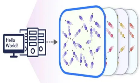
MLAutotuningHPC – Smart ensembles
Here we choose the best strategy to achieve some
computation goal such as providing the most efficient training
set with defining parameters spread well over the relevant phase
space. Ensembles are also essential in many computational
studies such as weather forecasting or search for new drugs
where regions of defining parameters need to be searched. This
category overlaps with the following Learning Model Details
(effective potentials and coarse graining) category as both look
at the structure of the simulation. Different papers tackle related
but distinct goals. Some look for reaction coordinates that are
collective variables (CV) that can be used to accelerate the
simulation; these are typically the slowest varying with time
modes of the system. Others look for structure (order
parameters) of the system such as “has the protein folded”.
Fig. 5. MLAutotuningHPC – Smart ensembles
1)
General Simulations-MLAutotuningHPC – Smart
ensembles
11.
Use of visualization to control smart ensembles of
simulations [27]
2)
Particle Dynamics-MLAutotuningHPC – Smart
ensembles
[image:3.612.329.561.454.591.2]13.
Use of machine learning to guide molecular dynamics
simulations to explore full range of phase space [29].
Manifold learning is used to find a low dimension set of
collective variables and then to learn dynamics in those
variables.
14.
Use of Machine Learning (Best Arm Identification
method) to optimize determination of protein-ligand
binding (docking) energies when total compute resources
are constrained, [30]
15.
Efficient exploration of configuration space by adding an
adaptively computed biasing potential using machine
learning to the original dynamics. [31]–[35]
16.
Use of the “information Bottleneck” approach to design
an ANN that will identify a collective coordinate that will
guide simulations with importance sampling to correct
bias [36], [37].This leads to a collective coordinator with
good physical (chemical) interpretation.
17.
Loop over multiple molecular dynamics and Deep
Learning steps to more accurately sample phase for long
time computations - termed “Reweighted autoencoded
variational Bayes for enhanced sampling (RAVE)” [38],
[39]
18.
Use reinforcement learning to learn a ANN representation
of the Free Energy based on an uncertainty estimate
comping from a set of ANN’s with the same updates and
different random starting weights [40]. The choice of
collective variables (CV) is not discussed except to note
that approach can accommodate a quite large number
(10-20) of CV’s.
19.
Study of protein folding using machine learning to
identify the special regions of phase space where proteins
do indeed fold [41], [42]. Google’s Alphafold [43], [44]
won [45] the 13th Critical Assessment of Structure
Prediction (CASP) competition [46] with deep learning
used to identify how specific proteins fold. Such studies
can be followed up by traditional MD simulations. In [47]
convolutions and a variational autoencoder (CVAE) are
used for dimension reduction to identify folding region.
3)
ABM-MLAutotuningHPC – Smart ensembles
20.
Smart ensembles for cancer agent-based models with
PhysiCell. [48]
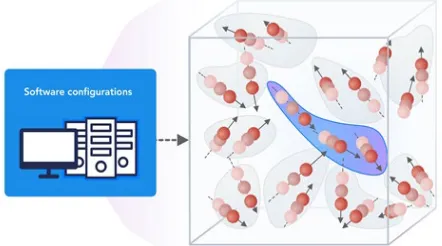
B.
MLaroundHPC: Learning Model Details (effective
potentials and coarse graining)
This is classic coarse graining strategy with recently, deep
learning replacing dimension reduction techniques.) One can
learn effective potentials and interaction graphs. An effective
potential is an analytic, empirical or
quasi-phenomenological potential that combines multiple, perhaps
opposing, effects into a single potential.
1)
Particle Dynamics-MLaroundHPC: Learning Model
Details (effective potentials)
21.
Use of machine learning to generate an effective
Hamiltonian using initial local updates as training data to
choose correlated update spins with Wolff’s method near
a critical point [49]. This is applied in [50]
22.
Neural-network representation [51]–[54] of DFT
potential-energy surfaces
23.
General framework for calculating a many-body
coarse-grained potential. [55]
24.
Formulate coarse-graining as a supervised machine
learning problem and use coarse-graining error and
cross-validation to select and compare the performance of
different models. [56]
25.
Review of the use of neural networks to represent
potentials and speed up simulations [57]. Has plot of
physics, chemistry and materials papers per year using
ANN’s. There are 1500 per year after 2010.
2)
Particle Dynamics-MLaroundHPC: Learning Model
Details (coarse graining)
26.
VAMP(variational approach for Markov processes)nets to
learn end to end reduced complexity surrogates of
molecular dynamics without custom modelling such as
transformation of simulated coordinates into structural
features, dimension reduction, clustering the
dimension-reduced data, and estimation of a Markov state models
[58]
27.
Use of collective variables (dimension reduction) to study
protein dynamics [59]
28.
Obtains one-dimensional collective variables for studying
rarely occurring transitions between two metastable states
separated by a high free energy barrier [60].
29.
Collective variables to sample molecular dynamics and
free energy landscape using autoencoders [61]–[64].
Includes MLAutotuningHPC – Smart ensembles
30.
Use of machine learning to support long time scale
molecular simulations [65] Reviews other approaches
such as RAVE and VAMP. Includes MLAutotuningHPC
– Smart ensembles.
3)
PDE-MLaroundHPC: Learning Model Details (coarse
graining)
31.
Use of equation free modeling [66] for coarse graining
combined with manifold learning (dimension reduction)
[67]
[image:4.612.318.539.551.674.2]32.
Uses neural nets as expansion functions for solutions of
partial differential equations [68].
C.
MLaroundHPC: Learning Model Details - Inference of
Missing Model Structure
[image:5.612.57.283.225.376.2]The final category in the Structure, Theory and Model class
and represented in the above figure imagines a future where AI
will essentially be able to derive theories from data, or more
practically a mix of data and models. This is especially
promising in agent based models which often contain
phenomenological approaches such as the predictor-corrector
method of sec. 2.1.3. We expect that will take the results of such
assimilation and effective potentials and interactions discussed
earlier and use them as the master model or theory for future
research.
Fig. 7. MLaroundHPC: Learning Model Details - Inference of Missing Model Structure
IV.
T
AXONOMY OFMLA
UTOTUNING ANDML
AROUNDHPC:
L
EARNS
URROGATES FORS
IMULATIONA.
MLaroundHPC: Learning Outputs from Inputs: a)
Computation Results from Computation defining
Parameters
Fig. 8. MLaroundHPC: Learning Outputs from Inputs: Computation Results from Computation defining Parameters
In this category, one just feeds in a modest number of
meta-parameters that define the problem and learn a modest number
of calculated answers. In many circumstances, summary
parameters are joined with observed properties to specify
compounds. This task presumably requires fewer training
samples than “fields from fields” (next category) and is main
MLaroundHPC use so far.
Operationally this category is the same as
SimulationTrainedML but with a different goal: In
SimulationTrainedML the simulations are performed to directly
train an AI system rather than the case here where the AI system
is being added to learn a simulation.
1)
Particle Dynamics- MLaroundHPC: Learning Outputs
from Inputs (parameters)
33.
An early paper in 2012 using non-ANN machine learning
to learn energies from molecular properties [69]
34.
Use of generative and predictive ANN to predict drug
properties from their SMILES representation using
existing databases [70].Use of DNN to learn crystal
energies and stability with training data calculated by
DFT. [71]
35.
Review of machine learning (emphasized) for molecular
and materials science [72]
36.
Nanoparticle simulations [73] defining surrogates learnt
as a function of defining parameters
37.
Review article on machine learning to predict material
properties from structure of compounds. Uses observation
and simulations to determine structure-property
relationships for training [74]
38.
Use of neural nets to describe potentials and simulation
results for Infrared Spectra [75] The input features to the
ANN’s are the parameters of Frenkel exciton
Hamiltonians and the output average exciton transfer
times and overall transfer efficiencies.
39.
Machine Learning (kernel ridge regression) to map
database (of DFT simulations) into material properties.
[76]
40.
Machine Learning (kernel ridge regression) to map
database (of DFT simulations) into valence charge
densities. [77], [78]
41.
ANN’s for fast estimate of excitation energy transfer
properties (used in solar cells) [79]. The ANN is used to
map Hamiltonian specifications into material properties.
42.
Machine Learning to predict the energies and forces and
avoid repetitive computations [80]. A decision engine
decides whether to use learnt result or calculate using full
simulation.
43.
Machine Learning used to estimate forces in molecular
simulations choosing between ab initio Quantum
mechanics or regression based ML estimate from a
database enhanced dynamically. [32], [81]
44.
Review of machine learning with dimensionality
reduction and clustering algorithms, drug discovery
DeepTox, free-energy surface of molecules, ligand
binding site detection, ligand pose prediction, ligand,
active/inactive classification, ligand binding affinity
prediction, and protein design, DeepChem software,
MoleculeNet challenge and access to relevant QSAR
prediction datasets. Two cases covered in detail - ML
representation of Quantum forces and prediction of
binding affinities. [82]
[image:5.612.52.294.491.595.2]intermediate size. Focus on use of a particular
representation of input molecular structure [83].
46.
Specifying atom representations for input into machine
learning [84]
47.
MLaroundHPC: Learning Outputs from Inputs
(parameters)
is reviewed but generalized to learn system
wavefunction in its hamiltonian matrix element form
allowing richer set of predictions with
MLaroundHPC:
Learning Outputs from Inputs (fields)
[85]
2)
PDE-MLaroundHPC - Learning Outputs from Inputs
(parameters)
48.
Finding coefficients of a PDE that reproduce observed
data [86]
49.
Machine Learning surrogates of heart simulations to
speed up aortic aneurysm studies [87]
B.
MLaroundHPC: Learning Outputs from Inputs: b) Fields
[image:6.612.51.271.284.419.2]from Fields
Fig. 9. MLaroundHPC: b) Learning Outputs from Inputs: Fields from Fields
Here one feeds in initial conditions and the neural network
learns the result where initial and final results are fields
There is also a mixed category c) Learning Outputs from
Inputs: output fields from computation defining parameters
combining a) and b), which we don’t illustrate.
1)
Particle Dynamics-MLaroundHPC: Learning Outputs
from Inputs (fields)
50.
An early paper using in 1994 neural nets to solve ODE’s.
[88]]
51.
Investigation of different neural network structures to
learn the results of an Ising model simulation near its
critical point comparing with classic Monte Carlo using a
combination of single-site Metropolis and Wolff cluster
updates [89]
52.
MLaroundHPC: Learning Outputs from Inputs
(parameters) is reviewed but generalized to learn system
wavefunction in its hamiltonian matrix element form
allowing richer set of predictions with MLaroundHPC:
Learning Outputs from Inputs (fields) [85]
53.
Using Generative Adversarial Networks to produce
surrogates of large scale simulations of the effect of
gravitational lensing used to study early universe
CosmoGAN [90], [91] with supplement [92] on Github
54.
Uses LSTM’s to learn time series represented by
molecular dynamics simulation [93]. Promising results on
small model systems.
55.
Uses deep learning to find a clean set of collective
coordinates that can be easily sampled to efficiently move
through phase space [94].
2)
ABM-MLaroundHPC: Learning Outputs from Inputs
(fields)
56.
Use of Deep Learning LSTM to produce surrogates of a
one-dimensional biological agent simulation [95]. Errors
were estimated by training four neural networks differing
in initial (random) choices of weights. 105 simulations
took 2 months on a 400 node cluster and were followed
by looking at 108 surrogate runs for an in depth survey
over the full phase space. The speedup was 30,000 using
surrogates.
57.
Deep Learning for Agent-based Epidemic Forecasting
DEFSI with ANN’s learning detailed (county level)
information from simulations. [96]
3)
PDE-MLaroundHPC: Learning Outputs from Inputs
(fields)
58.
Finding forward (direct) and inverse mapping functions of
input to output. The inverse map is particularly interesting
as it is no harder than direct method for ANN’s but classic
PDE solvers only give direct map straightforwardly. [97],
[98]
59.
Deep Learning for solving partial differential equations
[99], [100] (called Physics Informed Neural Net PINN)
extended to nonlinear systems [101]
60.
Uses PINN to solve stochastic forward and inverse
problems with separate DNN to learn error. [102]
61.
Deep learning to find surrogates for fluid flow
simulations [103]
62.
Use of machine learning to improve Extended dynamic
mode decomposition for representing Koopman Operator
to represent dynamical systems. The ANN learns the
operators used to represent the solution.[104]
63.
Solving high dimensional (up to 1000’s) partial
differential equations using deep learning surrogates with
differentiation of neural net form and no mesh points.
Exact solutions used to train surrogates [105], [106]
64.
Explicitly differentiating the ANN in [87] solving
advection and diffusion type PDEs in complex
geometries[107]
V.
C
ONCLUSIONSmethods into the 8 categories, one can expect them all to be
combined in future projects as illustrated in fig. 10.
Fig. 10.8 MLAutotuning and MLaroundHPC appoaches combined.
Acknowledgements
Partial support by NSF CIF21 DIBBS 1443054, NSF nanoBIO
1720625, NSF CINES 1835598 and NSF BDEC2 1849625 is
gratefully acknowledged. We thank the “Learning
Everywhere” collaboration James A. Glazier, JCS Kadupitiya,
Vikram Jadhao, Minje Kim, Judy Qiu, James P. Sluka, Endre
Somogyi, Madhav Marathe, Abhijin Adiga, Jiangzhuo Chen,
and Oliver Beckstein for many discussions. SJ is partially
supported by DOE ECP “ExaLearn”.
R
EFERENCES[1] Geoffrey Fox, James A. Glazier, JCS Kadupitiya, Vikram Jadhao, Minje Kim, Judy Qiu, James P. Sluka, Endre Somogyi, Madhav Marathe, Abhijin Adiga, Jiangzhuo Chen, Oliver Beckstein, and Shantenu Jha, “Learning Everywhere: Pervasive Machine Learning for Effective High-Performance Computation,” presented at the HPDC Workshop at IPDPS, Rio de Janeiro [Online]. Available: https://arxiv.org/abs/1902.10810, http://dsc.soic.indiana.edu/publications/Learning_Everywhere_Summar y.pdf
[2] Geoffrey Fox, James A. Glazier, JCS Kadupitiya, Vikram Jadhao, Minje Kim, Judy Qiu, James P. Sluka, Endre Somogyi, Madhav Marathe, Abhijin Adiga, Jiangzhuo Chen, Oliver Beckstein, and Shantenu Jha, “Learning Everywhere: Pervasive Machine Learning for Effective High-Performance Computation: Application Background,” Feb. 2019
[Online]. Available: http://dsc.soic.indiana.edu/publications/Learning_Everywhere.pdf
[3] Geoffrey Fox, Shantenu Jha, “Understanding ML driven HPC: Applications and Infrastructure,” in IEEE eScience 2019 Conference, San Diego, California [Online]. Available: https://escience2019.sdsc.edu/ [4] Geoffrey Fox, Shantenu Jha, “Learning Everywhere: A Taxonomy for the
Integration of Machine Learning and Simulations,” in IEEE eScience 2019 Conference, San Diego, California [Online]. Available: https://escience2019.sdsc.edu/
[5] Geoffrey Fox, Shantenu Jha, “The Promise of Learning Everywhere and MLforHPC,” in Online Resource for BDEC2 Second Meeting at Kobe Japan, Kobe Japan [Online]. Available:
http://dsc.soic.indiana.edu/presentations/JhaFox_BDEC2_Kobe_02-2019.pptx
[6] Shantenu Jha, Geoffrey Fox, “Presentation: Learning Everywhere: Pervasive Machine Learning for Effective High-Performance Computing,” presented at the HPBDC workshop at IPDPS Conference, Rio de Janeiro, Brazil, 2019 [Online]. Available: http://dsc.soic.indiana.edu/presentations/LE-ipdps19.pdf. [Accessed: 07-Jun-2019]
[7] Jeff Dean, “Machine Learning for Systems and Systems for Machine Learning,” in Presentation at 2017 Conference on Neural Information
Processing Systems, Long Beach, CA [Online]. Available: http://learningsys.org/nips17/assets/slides/dean-nips17.pdf
[8] Microsoft Research, “AI for AI Systems at Microsoft Faculty Summit,” August 1-2 2018. [Online]. Available: https://youtu.be/MqBOuoLflpU. [Accessed: 29-Jan-2019]
[9] Microsoft Research, “AI for Database and Data Analytic Systems at Microsoft Faculty Summit,” August 1-2, 2018. [Online]. Available: https://youtu.be/Tkl6ERLWAbA. [Accessed: 29-Jan-2019]
[10] S. Matsuoka, “Post-K: A Game Changing Supercomputer for Convergence of HPC and Big Data / AI,” 13-Feb-2019 [Online]. Available: https://drive.google.com/file/d/1t_F_shSU-48uDh4FKHhpZQXWIhk-BgJX/view?usp=sharing
[11] G. Fox, D. Crandall, J. Qiu, G. Von Laszewski, S. Jha, J. Paden, O. Beckstein, T. Cheatham, M. Marathe, and F. Wang, “NSF 1443054: CIF21 DIBBs: Middleware and High Performance Analytics Libraries for Scalable Data Science, Poster,” presented at the DIBBs18 NSF Workshop, Data Infrastructure Building Blocks (DIBBs) https://dibbs18.ucsd.edu/, Washington DC, 2018 [Online]. Available: http://dsc.soic.indiana.edu/presentations/SPIDALPosterDibbsNSF14430 54_0622.pdf
[12] O. Beckstein, G. Fox, J. Qiu, D. Crandall, G. von Laszewski, J. Paden, S. Jha, F. Wang, M. Marathe, A. Vullikanti, and T. Cheatham, “Contributions to High-Performance Big Data Computing,” Sep. 2018
[Online]. Available: http://dsc.soic.indiana.edu/publications/SPIDALPaperSept2018.pdf
[13] Geoffrey Fox, “HPC, Big Data, and Machine Learning Convergence,” Presentation Washington DC, 17-Jul-2019. [Online]. Available:
http://dsc.soic.indiana.edu/presentations/HPC-BigDataConvergenceJuly16-2019.pdf
[14] JCS Kadupitiya, Geoffrey C. Fox, Vikram Jadhao, “Machine Learning for Parameter Auto-tuning in Molecular Dynamics Simulations: Efficient Dynamics of Ions near Polarizable Nanoparticles,” Indiana University,
Nov. 2018 [Online]. Available: http://dsc.soic.indiana.edu/publications/Manuscript.IJHPCA.Nov2018.p
df
[15] C. J. Pretorius, M. C. du Plessis, and C. B. Cilliers, “Simulating Robots Without Conventional Physics: A Neural Network Approach,” J. Intell. Rob. Syst., vol. 71, no. 3–4, pp. 319–348, Sep. 2013 [Online]. Available: https://link.springer.com/article/10.1007/s10846-012-9782-6. [Accessed: 21-Jul-2019]
[16] F. Lamperti, A. Roventini, and A. Sani, “Agent-based model calibration using machine learning surrogates,” J. Econ. Dyn. Control, vol. 90, pp. 366–389, May 2018 [Online]. Available: http://www.sciencedirect.com/science/article/pii/S0165188918301088
[17] M. H. Zangooei and J. Habibi, “Hybrid multiscale modeling and prediction of cancer cell behavior,” PLoS One, vol. 12, no. 8, p. e0183810, Aug. 2017 [Online]. Available: http://dx.doi.org/10.1371/journal.pone.0183810
[18] B. C. Daniels, W. S. Ryu, and I. Nemenman, “Automated, predictive, and interpretable inference of Caenorhabditis elegans escape dynamics,” Proc. Natl. Acad. Sci. U. S. A., vol. 116, no. 15, pp. 7226–7231, Apr. 2019 [Online]. Available: http://dx.doi.org/10.1073/pnas.1816531116 [19] B. C. Daniels and I. Nemenman, “Automated adaptive inference of
phenomenological dynamical models,” Nat. Commun., vol. 6, p. 8133, Aug. 2015 [Online]. Available: http://dx.doi.org/10.1038/ncomms9133 [20] B. C. Daniels and I. Nemenman, “Automated adaptive inference of
coarse-grained dynamical models in systems biology,” arXiv [q-bio.QM], 24-Apr-2014 [Online]. Available: http://arxiv.org/abs/1404.6283 [21] J. Lagergren, J. T. Nardini, G. Michael Lavigne, E. M. Rutter, and K. B.
Flores, “Learning partial differential equations for biological transport models from noisy spatiotemporal data,” arXiv [math.DS], 13-Feb-2019 [Online]. Available: http://arxiv.org/abs/1902.04733
[22] X. Geng, X. Wu, L. Zhang, Q. Yang, Y. Liu, and J. Ye, “Multi-Modal Graph Interaction for Multi-Graph Convolution Network in Urban Spatiotemporal Forecasting,” arXiv [cs.LG], 27-May-2019 [Online]. Available: http://arxiv.org/abs/1905.11395
Syst Biol Appl, vol. 4, p. 19, May 2018 [Online]. Available: http://dx.doi.org/10.1038/s41540-018-0054-3
[24] Y. Wu, Y. Yang, H. Nishiura, and M. Saitoh, “Deep Learning for Epidemiological Predictions,” in The 41st International ACM SIGIR Conference on Research & Development in Information Retrieval, 2018,
pp. 1085–1088 [Online]. Available: https://dl.acm.org/citation.cfm?id=3209978.3210077. [Accessed:
08-Jun-2019]
[25] S. R. Venna, A. Tavanaei, R. N. Gottumukkala, V. V. Raghavan, A. S. Maida, and S. Nichols, “A Novel Data-Driven Model for Real-Time Influenza Forecasting,” IEEE Access, vol. 7, pp. 7691–7701, 2019 [Online]. Available: http://dx.doi.org/10.1109/ACCESS.2018.2888585 [26] S. Rasp, M. S. Pritchard, and P. Gentine, “Deep learning to represent
subgrid processes in climate models,” Proc. Natl. Acad. Sci. U. S. A., vol. 115, no. 39, p. 9684, Sep. 2018 [Online]. Available: http://www.pnas.org/content/115/39/9684.abstract
[27] K. Matković, D. Gračanin, and H. Hauser, “Visual Analytics for Simulation Ensembles,” in Proceedings of the 2018 Winter Simulation Conference, Gothenburg, Sweden, 2018, pp. 321–335 [Online]. Available: http://dl.acm.org/citation.cfm?id=3320516.3320563
[28] P. M. Kasson and S. Jha, “Adaptive ensemble simulations of biomolecules,” arXiv [q-bio.QM], 13-Sep-2018 [Online]. Available: http://arxiv.org/abs/1809.04804
[29] E. Chiavazzo, R. Covino, R. R. Coifman, C. W. Gear, A. S. Georgiou, G. Hummer, and I. G. Kevrekidis, “Intrinsic map dynamics exploration for uncharted effective free-energy landscapes,” Proc. Natl. Acad. Sci. U. S. A., vol. 114, no. 28, pp. E5494–E5503, Jul. 2017 [Online]. Available: http://dx.doi.org/10.1073/pnas.1621481114
[30] K. Terayama, H. Iwata, M. Araki, Y. Okuno, and K. Tsuda, “Machine learning accelerates MD-based binding pose prediction between ligands and proteins,” Bioinformatics, vol. 34, no. 5, pp. 770–778, Mar. 2018 [Online]. Available: https://www.ncbi.nlm.nih.gov/pubmed/29040432 [31] R. Galvelis and Y. Sugita, “Neural Network and Nearest Neighbor
Algorithms for Enhancing Sampling of Molecular Dynamics,” J. Chem. Theory Comput., vol. 13, no. 6, pp. 2489–2500, Jun. 2017 [Online]. Available: http://dx.doi.org/10.1021/acs.jctc.7b00188
[32] A. Z. Guo, E. Sevgen, H. Sidky, J. K. Whitmer, J. A. Hubbell, and J. J. de Pablo, “Adaptive enhanced sampling by force-biasing using neural networks,” J. Chem. Phys., vol. 148, no. 13, p. 134108, Apr. 2018 [Online]. Available: http://dx.doi.org/10.1063/1.5020733
[33] H. Sidky and J. K. Whitmer, “Learning free energy landscapes using artificial neural networks,” J. Chem. Phys., vol. 148, no. 10, p. 104111, Mar. 2018 [Online]. Available: http://dx.doi.org/10.1063/1.5018708 [34] Jun Zhang, Yi Isaac Yang, and Frank Noé, “Targeted Adversarial
Learning Optimized Sampling,” May 2019 [Online]. Available: https://chemrxiv.org/articles/Targeted_Adversarial_Learning_Optimized _Sampling/7932371
[35] E. Schneider, L. Dai, R. Q. Topper, C. Drechsel-Grau, and M. E. Tuckerman, “Stochastic Neural Network Approach for Learning High-Dimensional Free Energy Surfaces,” Phys. Rev. Lett., vol. 119, no. 15, p. 150601, Oct. 2017 [Online]. Available: http://dx.doi.org/10.1103/PhysRevLett.119.150601
[36] Y. Wang, J. Ribeiro, and P. Tiwary, “Past-future information bottleneck framework for simultaneously sampling biomolecular reaction coordinate, thermodynamics and kinetics,” BioRxiv, p. 507822, 2018
[Online]. Available: https://www.biorxiv.org/content/10.1101/507822v1.abstract
[37] Y. Wang, J. M. L. Ribeiro, and P. Tiwary, “Past–future information bottleneck for sampling molecular reaction coordinate simultaneously with thermodynamics and kinetics,” Nat. Commun., vol. 10, no. 1, p. 3573, Aug. 2019 [Online]. Available: https://doi.org/10.1038/s41467-019-11405-4
[38] J. M. Lamim Ribeiro and P. Tiwary, “Toward Achieving Efficient and Accurate Ligand-Protein Unbinding with Deep Learning and Molecular Dynamics through RAVE,” J. Chem. Theory Comput., vol. 15, no. 1, pp. 708–719, Jan. 2019 [Online]. Available: http://dx.doi.org/10.1021/acs.jctc.8b00869
[39] J. M. L. Ribeiro, P. Bravo, Y. Wang, and P. Tiwary, “Reweighted autoencoded variational Bayes for enhanced sampling (RAVE),” J.
Chem. Phys., vol. 149, no. 7, p. 072301, Aug. 2018 [Online]. Available: http://dx.doi.org/10.1063/1.5025487
[40] L. Zhang, H. Wang, and E. Weinan, “Reinforced dynamics for enhanced sampling in large atomic and molecular systems,” J. Chem. Phys., vol. 148, no. 12, p. 124113, Mar. 2018 [Online]. Available: http://dx.doi.org/10.1063/1.5019675
[41] M. Gao, H. Zhou, and J. Skolnick, “DESTINI: A deep-learning approach to contact-driven protein structure prediction,” Sci. Rep., vol. 9, no. 1, p. 3514, Mar. 2019 [Online]. Available: http://dx.doi.org/10.1038/s41598-019-40314-1
[42] N. Anand and P. Huang, “Generative modeling for protein structures,” in Advances in Neural Information Processing Systems 31, S. Bengio, H. Wallach, H. Larochelle, K. Grauman, N. Cesa-Bianchi, and R. Garnett, Eds. Curran Associates, Inc., 2018, pp. 7494–7505 [Online]. Available: http://papers.nips.cc/paper/7978-generative-modeling-for-protein-structures.pdf
[43] Google Deepmind, “AlphaFold: Using AI for scientific discovery,” 02-Dec-2018. [Online]. Available: https://deepmind.com/blog/alphafold/. [Accessed: 02-Aug-2019]
[44] R. Evans, J. Jumper, J. Kirkpatrick, L. Sifre, T. F. G. Green, C. Qin, A. Zidek, A. Nelson, A. Bridgland, H. Penedones, S. Petersen, K. Simonyan, S. Crossan, D. T. Jones, D. Silver, et al., “De novo structure prediction with deep-learning based scoring” [Online]. Available: https://deepmind.com/documents/262/A7D_AlphaFold.pdf
[45] Robert F. Service, “Google’s DeepMind aces protein folding,”
06-Dec-2018. [Online]. Available:
https://www.sciencemag.org/news/2018/12/google-s-deepmind-aces-protein-folding. [Accessed: 18-Aug-2018]
[46] “13th Community Wide Experiment on the Critical Assessment of Techniques for Protein Structure Prediction CASP.” [Online]. Available: http://www.predictioncenter.org/casp13/index.cgi. [Accessed: 18-Aug-2019]
[47] Heng Ma, Debsindhu Bhowmik, Hyungro Lee, Matteo Turilli, Michael T. Young, Shantenu Jha, Arvind Ramanathan, “Deep Generative Model Driven Protein Folding Simulation,” Aug. 2019 [Online]. Available: https://arxiv.org/abs/1908.00496
[48] J. Ozik, N. Collier, R. Heiland, G. An, and P. Macklin, “Learning-accelerated Discovery of Immune-Tumour Interactions,” bioRxiv, p. 573972, Jan. 2019 [Online]. Available: http://biorxiv.org/content/early/2019/04/15/573972.abstract
[49] Z. Y. Meng, J. Liu, Y. Qi, and L. Fu, “Self-learning Monte Carlo method,” Physical Review B, vol. 95, no. 041101, Jan. 2017 [Online]. Available: https://dspace.mit.edu/handle/1721.1/106311. [Accessed: 08-Jun-2019] [50] X. Y. Xu, Z. H. Liu, G. Pan, Y. Qi, K. Sun, and Z. Y. Meng, “Revealing
Fermionic Quantum Criticality from New Monte Carlo Techniques,” arXiv [cond-mat.str-el], 15-Apr-2019 [Online]. Available: http://arxiv.org/abs/1904.07355
[51] J. S. Smith, O. Isayev, and A. E. Roitberg, “ANI-1: an extensible neural network potential with DFT accuracy at force field computational cost,” Chem. Sci., vol. 8, no. 4, pp. 3192–3203, Apr. 2017 [Online]. Available: http://dx.doi.org/10.1039/c6sc05720a
[52] J. S. Smith, B. Nebgen, N. Lubbers, O. Isayev, and A. E. Roitberg, “Less is more: Sampling chemical space with active learning,” J. Chem. Phys., vol. 148, no. 24, p. 241733, Jun. 2018 [Online]. Available: http://dx.doi.org/10.1063/1.5023802
[53] J. S Smith, B. T. Nebgen, R. Zubatyuk, N. Lubbers, C. Devereux, K. Barros, S. Tretiak, O. Isayev, and A. Roitberg, “Outsmarting quantum chemistry through transfer learning,” 2018 [Online]. Available: https://chemrxiv.org/articles/Outsmarting_Quantum_Chemistry_Throug h_Transfer_Learning/6744440/files/12304376.pdf
[54] J. Behler and M. Parrinello, “Generalized neural-network representation of high-dimensional potential-energy surfaces,” Phys. Rev. Lett., vol. 98, no. 14, p. 146401, Apr. 2007 [Online]. Available: http://dx.doi.org/10.1103/PhysRevLett.98.146401
[56] J. Wang, S. Olsson, C. Wehmeyer, A. Pérez, N. E. Charron, G. de Fabritiis, F. Noé, and C. Clementi, “Machine Learning of Coarse-Grained Molecular Dynamics Force Fields,” ACS Cent. Sci., vol. 5, no. 5, pp. 755–767, May 2019 [Online]. Available: https://doi.org/10.1021/acscentsci.8b00913
[57] J. Behler, “First Principles Neural Network Potentials for Reactive Simulations of Large Molecular and Condensed Systems,” Angew. Chem. Int. Ed Engl., vol. 56, no. 42, pp. 12828–12840, Oct. 2017 [Online]. Available: http://dx.doi.org/10.1002/anie.201703114
[58] A. Mardt, L. Pasquali, H. Wu, and F. Noé, “VAMPnets for deep learning of molecular kinetics,” Nat. Commun., vol. 9, no. 1, p. 5, Jan. 2018 [Online]. Available: http://dx.doi.org/10.1038/s41467-017-02388-1 [59] F. Sittel and G. Stock, “Perspective: Identification of collective variables
and metastable states of protein dynamics,” J. Chem. Phys., vol. 149, no. 15, p. 150901, Oct. 2018 [Online]. Available: http://dx.doi.org/10.1063/1.5049637
[60] D. Mendels, G. Piccini, and M. Parrinello, “Collective Variables from Local Fluctuations,” J. Phys. Chem. Lett., vol. 9, no. 11, pp. 2776–2781,
Jun. 2018 [Online]. Available: http://dx.doi.org/10.1021/acs.jpclett.8b00733
[61] W. Chen and A. L. Ferguson, “Molecular enhanced sampling with autoencoders: On-the-fly collective variable discovery and accelerated free energy landscape exploration,” arXiv [physics.bio-ph], 30-Dec-2017 [Online]. Available: http://arxiv.org/abs/1801.00203
[62] W. Chen, A. R. Tan, and A. L. Ferguson, “Collective variable discovery and enhanced sampling using autoencoders: Innovations in network architecture and error function design,” J. Chem. Phys., vol. 149, no. 7, p. 072312, Aug. 2018 [Online]. Available: http://dx.doi.org/10.1063/1.5023804
[63] M. M. Sultan, H. K. Wayment-Steele, and V. S. Pande, “Transferable Neural Networks for Enhanced Sampling of Protein Dynamics,” J. Chem. Theory Comput., vol. 14, no. 4, pp. 1887–1894, Apr. 2018 [Online]. Available: http://dx.doi.org/10.1021/acs.jctc.8b00025
[64] C. Wehmeyer and F. Noé, “Time-lagged autoencoders: Deep learning of slow collective variables for molecular kinetics,” J. Chem. Phys., vol. 148, no. 24, p. 241703, Jun. 2018 [Online]. Available: http://dx.doi.org/10.1063/1.5011399
[65] F. Noé, “Machine Learning for Molecular Dynamics on Long Timescales,” arXiv [physics.chem-ph], 18-Dec-2018 [Online]. Available: http://arxiv.org/abs/1812.07669
[66] I. G. Kevrekidis, C. W. Gear, and G. Hummer, “Equation-free: The computer-aided analysis of complex multiscale systems,” AIChE J., vol. 50, no. 7, pp. 1346–1355, 2004 [Online]. Available: https://onlinelibrary.wiley.com/doi/abs/10.1002/aic.10106
[67] I. G. Kevrekidis, “Equation-free and variable free modeling for complex/multiscale systems. Coarse-grained computation in science and engineering using fine-grained models,” Princeton Univ., NJ (United States), DOE-PRINCETON-25877, Feb. 2017 [Online]. Available: https://www.osti.gov/biblio/1347549-equation-free-variable-free- modeling-complex-multiscale-systems-coarse-grained-computation-science-engineering-using-fine-grained-models. [Accessed: 09-Jun-2019]
[68] Esteban Samaniego, Cosmin Anitescu, Somdatta Goswami, Vien Minh Nguyen-Thanh, Hongwei Guo, Khader Hamdia, Timon Rabczuk, Xiaoying Zhuang, “An Energy Approach to the Solution of Partial Differential Equations in Computational Mechanics via Machine Learning: Concepts, Implementation and Applications,” arXiv [stat.ML], , 27 Aug 2019 [Online]. Available: https://arxiv.org/abs/1908.10407 [69] M. Rupp, A. Tkatchenko, K.-R. Müller, and O. A. von Lilienfeld, “Fast
and accurate modeling of molecular atomization energies with machine learning,” Phys. Rev. Lett., vol. 108, no. 5, p. 058301, Feb. 2012 [Online]. Available: http://dx.doi.org/10.1103/PhysRevLett.108.058301
[70] M. Popova, O. Isayev, and A. Tropsha, “Deep reinforcement learning for de novo drug design,” Sci Adv, vol. 4, no. 7, p. eaap7885, Jul. 2018 [Online]. Available: http://dx.doi.org/10.1126/sciadv.aap7885
[71] W. Ye, C. Chen, Z. Wang, I.-H. Chu, and S. P. Ong, “Deep neural networks for accurate predictions of crystal stability,” Nat. Commun., vol. 9, no. 1, p. 3800, Sep. 2018 [Online]. Available: http://dx.doi.org/10.1038/s41467-018-06322-x
[72] K. T. Butler, D. W. Davies, H. Cartwright, O. Isayev, and A. Walsh, “Machine learning for molecular and materials science,” Nature, vol. 559, no. 7715, pp. 547–555, Jul. 2018 [Online]. Available: http://dx.doi.org/10.1038/s41586-018-0337-2
[73] JCS Kadupitiya , Geoffrey C. Fox , and Vikram Jadhao, “Machine learning for performance enhancement of molecular dynamics simulations,” presented at the International Conference on Computational Science ICCS2019 , Faro, Algarve, Portugal, 2018 [Online]. Available: http://dsc.soic.indiana.edu/publications/ICCS8.pdf
[74] P. V. Balachandran, “Machine learning guided design of functional materials with targeted properties,” Comput. Mater. Sci., vol. 164, pp. 82– 90, Jun. 2019 [Online]. Available: http://www.sciencedirect.com/science/article/pii/S0927025619301922
[75] M. Gastegger, J. Behler, and P. Marquetand, “Machine learning molecular dynamics for the simulation of infrared spectra,” Chem. Sci., vol. 8, no. 10, pp. 6924–6935, Oct. 2017 [Online]. Available: http://dx.doi.org/10.1039/c7sc02267k
[76] A. P. Bartók, S. De, C. Poelking, N. Bernstein, J. R. Kermode, G. Csányi, and M. Ceriotti, “Machine learning unifies the modeling of materials and molecules,” Sci Adv, vol. 3, no. 12, p. e1701816, Dec. 2017 [Online]. Available: http://dx.doi.org/10.1126/sciadv.1701816
[77] A. Grisafi, A. Fabrizio, B. Meyer, D. M. Wilkins, C. Corminboeuf, and M. Ceriotti, “Transferable Machine-Learning Model of the Electron Density,” ACS Cent Sci, vol. 5, no. 1, pp. 57–64, Jan. 2019 [Online]. Available: http://dx.doi.org/10.1021/acscentsci.8b00551
[78] A. Grisafi, D. M. Wilkins, G. Csányi, and M. Ceriotti, “Symmetry-Adapted Machine Learning for Tensorial Properties of Atomistic Systems,” Phys. Rev. Lett., vol. 120, no. 3, p. 036002, Jan. 2018 [Online]. Available: http://dx.doi.org/10.1103/PhysRevLett.120.036002
[79] F. Häse, C. Kreisbeck, and A. Aspuru-Guzik, “Machine learning for quantum dynamics: deep learning of excitation energy transfer properties,” Chem. Sci., vol. 8, no. 12, pp. 8419–8426, Dec. 2017 [Online]. Available: http://dx.doi.org/10.1039/c7sc03542j
[80] V. Botu and R. Ramprasad, “Adaptive machine learning framework to accelerate ab initio molecular dynamics,” Int. J. Quantum Chem., vol. 115, no. 16, pp. 1074–1083, Aug. 2015 [Online]. Available: http://doi.wiley.com/10.1002/qua.24836
[81] Z. Li, J. R. Kermode, and A. De Vita, “Molecular dynamics with on-the-fly machine learning of quantum-mechanical forces,” Phys. Rev. Lett., vol. 114, no. 9, p. 096405, Mar. 2015 [Online]. Available: http://dx.doi.org/10.1103/PhysRevLett.114.096405
[82] A. Pérez, G. Martínez-Rosell, and G. De Fabritiis, “Simulations meet machine learning in structural biology,” Theory and simulation • Macromolecular assemblies, vol. 49, pp. 139–144, Apr. 2018 [Online]. Available:
http://www.sciencedirect.com/science/article/pii/S0959440X17301069 [83] K. T. Schütt, F. Arbabzadah, S. Chmiela, K. R. Müller, and A.
Tkatchenko, “Quantum-chemical insights from deep tensor neural networks,” Nat. Commun., vol. 8, p. 13890, Jan. 2017 [Online]. Available: http://dx.doi.org/10.1038/ncomms13890
[84] M. J. Willatt, F. Musil, and M. Ceriotti, “Atom-density representations for machine learning,” J. Chem. Phys., vol. 150, no. 15, p. 154110, Apr. 2019 [Online]. Available: https://doi.org/10.1063/1.5090481
[85] K. T. Schütt, M. Gastegger, A. Tkatchenko, K. -R. Müller, and R. J. Maurer, “Unifying machine learning and quantum chemistry -- a deep neural network for molecular wavefunctions,” arXiv [physics.chem-ph], 24-Jun-2019 [Online]. Available: http://arxiv.org/abs/1906.10033 [86] Y. Khoo, J. Lu, and L. Ying, “Solving parametric PDE problems with
artificial neural networks,” arXiv [math.NA], 11-Jul-2017 [Online]. Available: http://arxiv.org/abs/1707.03351
[87] L. Liang, M. Liu, C. Martin, J. A. Elefteriades, and W. Sun, “A machine learning approach to investigate the relationship between shape features and numerically predicted risk of ascending aortic aneurysm,” Biomech. Model. Mechanobiol., vol. 16, no. 5, pp. 1519–1533, Oct. 2017 [Online]. Available: http://dx.doi.org/10.1007/s10237-017-0903-9
[89] A. Morningstar and R. G. Melko, “Deep Learning the Ising Model Near Criticality,” J. Mach. Learn. Res., vol. 18, no. 163, pp. 1–17, 2018 [Online]. Available: http://jmlr.org/papers/v18/17-527.html. [Accessed: 08-Jun-2019]
[90] M. Mustafa, D. Bard, W. Bhimji, Z. Lukić, R. Al-Rfou, and J. Kratochvil, “CosmoGAN: creating high-fidelity weak lensing convergence maps using Generative Adversarial Networks,” arXiv [astro-ph.IM], 07-Jun-2017 [Online]. Available: http://arxiv.org/abs/1706.02390
[91] “Popular account of CosmoGAN: Training a neural network to study dark matter.” [Online]. Available: https://phys.org/news/2019-05-cosmogan-neural-network-dark.html. [Accessed: 08-Jun-2019]
[92] “Code is to accompany ‘Creating Virtual Universes Using Generative Adversarial Networks’ CosmoGAN manuscript.” [Online]. Available: https://github.com/MustafaMustafa/cosmoGAN. [Accessed: 08-Jun-2019]
[93] K. Endo, K. Tomobe, and K. Yasuoka, “Multi-step time series generator for molecular dynamics,” in Thirty-Second AAAI Conference on Artificial Intelligence, 2018 [Online]. Available: https://www.aaai.org/ocs/index.php/AAAI/AAAI18/paper/viewPaper/16 477
[94] F. Noé, S. Olsson, J. Köhler, and H. Wu, “Boltzmann Generators -- Sampling Equilibrium States of Many-Body Systems with Deep Learning,” arXiv [stat.ML], 04-Dec-2018 [Online]. Available: http://arxiv.org/abs/1812.01729
[95] S. Wang, F. Kai, N. Luo, Y. Cao, F. Wu, C. Zhang, K. A. Heller, and L. You, “Massive computational acceleration by using neural networks to emulate mechanism-based biological models,” bioRxiv, p. 559559,
03-Mar-2019 [Online]. Available: https://www.biorxiv.org/content/10.1101/559559v2. [Accessed:
06-Jun-2019]
[96] Lijing Wang, J Chen, and Madhav Marathe., “DEFSI : Deep Learning Based Epidemic Forecasting with Synthetic Information,” presented at the Thirty-Third AAAI Conference on Artificial Intelligence (AAAI-19), Hilton Hawaiian Village, Honolulu, Hawaii, USA [Online]. Available: https://www.researchgate.net/publication/328639130_DEFSI_Deep_Lea rning_Based_Epidemic_Forecasting_with_Synthetic_Information [97] Y. Khoo, J. Lu, and L. Ying, “Solving for high-dimensional committor
functions using artificial neural networks,” Publ. Res. Inst. Math. Sci., vol. 6, no. 1, p. 1, Oct. 2018 [Online]. Available: https://doi.org/10.1007/s40687-018-0160-2
[98] Y. Khoo and L. Ying, “SwitchNet: a neural network model for forward and inverse scattering problems,” arXiv [math.NA], 23-Oct-2018 [Online]. Available: http://arxiv.org/abs/1810.09675
[99] M. Raissi, P. Perdikaris, and G. E. Karniadakis, “Physics Informed Deep Learning (Part I): Data-driven Solutions of Nonlinear Partial Differential Equations,” arXiv [cs.AI], 28-Nov-2017 [Online]. Available: http://arxiv.org/abs/1711.10561
[100]M. Raissi, P. Perdikaris, and G. E. Karniadakis, “Physics Informed Deep Learning (Part II): Data-driven Discovery of Nonlinear Partial Differential Equations,” arXiv [cs.AI], 28-Nov-2017 [Online]. Available: http://arxiv.org/abs/1711.10566
[101]M. Raissi, “Deep Hidden Physics Models: Deep Learning of Nonlinear Partial Differential Equations,” J. Mach. Learn. Res., vol. 19, no. 25, pp. 1–24, 2018 [Online]. Available: http://jmlr.org/papers/v19/18-046.html. [Accessed: 08-Jun-2019]
[102]D. Zhang, L. Lu, L. Guo, and G. E. Karniadakis, “Quantifying total uncertainty in physics-informed neural networks for solving forward and inverse stochastic problems,” arXiv [math.AP], 21-Sep-2018 [Online]. Available: http://arxiv.org/abs/1809.08327
[103]W. Gentzsch, “Deep Learning for Fluid Flow Prediction in the Cloud.” 08-Dec-2018 [Online]. Available: https://www.linkedin.com/pulse/deep-learning-fluid-flow-prediction-cloud-wolfgang-gentzsch/. [Accessed: 01-Mar-2019]
[104]Q. Li, F. Dietrich, E. M. Bollt, and I. G. Kevrekidis, “Extended dynamic mode decomposition with dictionary learning: A data-driven adaptive spectral decomposition of the Koopman operator,” Chaos: An Interdisciplinary Journal of Nonlinear Science, vol. 27, no. 10, p. 103111, 2017 [Online]. Available: https://doi.org/10.1063/1.4993854
[105]J. Sirignano and K. Spiliopoulos, “DGM: A deep learning algorithm for solving partial differential equations,” J. Comput. Phys., vol. 375, pp. 1339–1364, Dec. 2018 [Online]. Available: http://www.sciencedirect.com/science/article/pii/S0021999118305527 [106]J. Han, A. Jentzen, and W. E, “Solving high-dimensional partial
differential equations using deep learning,” Proc. Natl. Acad. Sci. U. S. A., vol. 115, no. 34, pp. 8505–8510, Aug. 2018 [Online]. Available: http://dx.doi.org/10.1073/pnas.1718942115