Real time water simulation and rendering using features of the latest OpenGL capable graphics hardware

Retrospective Theses and Dissertations Iowa State University Capstones, Theses and Dissertations

2007

Real-time water simulation and rendering using

features of the latest OpenGL-capable graphics

hardware

Kenneth Edward Kopecky II

Iowa State University

Follow this and additional works at:https://lib.dr.iastate.edu/rtd

Part of theComputer Sciences Commons

This Thesis is brought to you for free and open access by the Iowa State University Capstones, Theses and Dissertations at Iowa State University Digital Repository. It has been accepted for inclusion in Retrospective Theses and Dissertations by an authorized administrator of Iowa State University Digital Repository. For more information, please [email protected].

Recommended Citation

Kopecky, Kenneth Edward II, "Real-time water simulation and rendering using features of the latest OpenGL-capable graphics hardware" (2007).Retrospective Theses and Dissertations. 14855.

by

Kenneth Edward Kopecky II

A thesis submitted to the graduate faculty

in partial fulfillment of the requirements for the degree of

MASTER OF SCIENCE

Major: Human-Computer Interaction

Program of Study Committee: Eliot Winer, Major Professor

James Oliver Chris Harding

Iowa State University

Ames, Iowa

2007

UMI Number: 1447545

1447545

2008

UMI Microform

Copyright

All rights reserved. This microform edition is protected against unauthorized copying under Title 17, United States Code.

ProQuest Information and Learning Company 300 North Zeeb Road

P.O. Box 1346

Ann Arbor, MI 48106-1346

Table of Contents

Chapter 1: Introduction

1

Chapter 2: Background

5

Chapter 3: Method Development

16

Chapter 4: Results and Discussion

34

Chapter 5: Summary and Conclusions

44

Bibliography

46

1

Chapter 1

Introduction

Water is arguably the most important substance to life on Earth. It makes up a significant

part of our body. We drink it, keep clean with it, and swim in it. Water can be seen in some

form nearly everywhere we go, from the kitchen sink to the Ocean. With the prevalence of

water in our lives, it is clear that water is involved with a great variety of computer

simulations and game environments. At the same time, however, it has proven to be

extremely difficult to create convincing simulated water on a computer. A variety of

strategies have been developed for simulating water in all the different forms it can be found:

oceans, lakes, rain, and even in a glass. These strategies must be tailored to the particular

situation to take into account the important aspects of the simulation while avoiding the

computational costs associated with the unimportant ones.

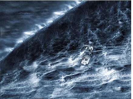
Water simulation is especially prevalent in the entertainment industry, most notably movies

and video games. Many famous movies, such as Titanic, Finding Nemo, and The Perfect

Storm (see figure 1) featured a great deal of computer-generated water. In the latter title,

many scenes were completely computer-rendered, but were indistinguishable from reality by

most moviegoers [1]. Video games, especially in the recent past, have begun allowing users

to explore and interact with mixed land-and-water environments. Whether destroying aliens

in a first-person shooter, riding a jet ski in a race, or catching fish in a more relaxed setting,

Figure 1: Simulated Water from A Perfect Storm

Outside of the entertainment industry, virtual water of a higher quality is used in simulations.

Computational fluid dynamics (CFD) can simulate water and other fluids effectively, and is

used for the design of everything from ventilation systems to boat hulls. For example, the

2008 German Olympic rowing team will be riding in boats that have been carefully

optimized using simulated water. [2]. While these simulations focus on the dynamics of the

water instead of the visual effects, the data they generate can be used to create water that both

3

The broad field of virtual reality (VR) is another important area where computer-generated

water is frequently used. For VR to be believable, the environments that are created must be

immersive and complete. Whether used for treating post-traumatic stress disorder, testing

out a new boat design, or just a brief escape from reality, bodies of water in VR applications

can add the necessary touch of immersion to turn a lackluster application into a truly

spectacular and effective one.

Speed Versus Realism

The different uses of water thus described all require different, and often specialized, types of

simulation. In fact, the primary difference between these simulations is the tradeoff between

computational speed and realism. For these purposes, there are two main categories of water

simulation: Pre-rendered and real-time. Pre-rendered water includes that used in movies and

scientific simulations. For the case of the German boat design, CFD is used to calculate the

most realistic water effects possible. These CFD simulations can take days to run, even on

modern computer clusters, and require very carefully configured inputs. In movies, a

different method is often used: procedural generation of the ocean surface. Movies such as

Titanic and WaterWorld used sections of water simulated by methods such as Fast Fourier

Transforms (FFTs) [29]. This and other methods for generating a water surface is less

computationally expensive than CFD, and their main objective is centered on visual appeal

more than absolute realism. The results of these water simulations are spectacular, and are

Conversely, real-time water is very different to handle. Unlike pre-rendered water, which can

take days or weeks of computation time to calculate only a few seconds of simulation,

real-time water must be updated many real-times per second. In fact, it is a misnomer of sorts to say

“real-time water”, because the term implies that one second of computation time is used to

calculate one second of simulation. In most situations, the computer is doing many things in

a single second to create the water simulation. To do this, real-time water simulators rely on a

greatly simplified model of water’s behavior and appearance. This real-time water is very

useful for adding realism and new interaction modes to games and simulations, which depend

on real-time effects exclusively. For example, real-time water in a game can allow the player

to use a boat that moves through a virtual world in a believable manner. Non-dynamic,

flat-shaded water is entirely doable and has been used in the past, but in today’s games and

simulations, a user demands believability and coherence of all elements of a scene.

The water rendering techniques discussed here, while not revolutionary, provide a foundation

to create realistic, simulated, interactive water in real-time. A complete package such as this

5

Chapter 2

Background

To investigate how best to imitate water, it is good to first look at the way that real water

works. The color and behavior of water depends almost completely on the environment in

which it is found. Oceans and lakes, for example, get their blue color both from reflections

of the sky and the diffusion of light beneath the water’s surface. [3]. Rivers and streams are

transparent or take on the color of the silt picked from the movement of the water. Ponds,

too, are either clear or cloudy from mud and other particles in the water.

The motion of water is also heavily dependent on its environment. Oceans and lakes are full

of waves that are caused by a variety of sources. While some of these waves are the result of

earthquakes, tidal forces, and moving ships, most waves are caused by wind moving across

the water’s surface [3]. The motion of rivers and streams comes from the interaction of the

flowing water with shores and bed of the river. Finally, ponds are fairly still unless the water

is stirred up slightly by wind or boats. All these types of water move differently and

Pre-rendered Water Simulation

For movies and other media that don’t need to be rendered in real-time, the highest-quality

rendering methods are used along with detailed simulation methods to create realistic,

believable water. For the behavior of this water, computational fluid dynamics methods are

often used. Another common method for simulating water accurately is smoothed particle

systems. Here [5], a physically simulated system of “water balls” is used as a virtual 3D

fluid. A closed surface surrounding the particles (hence the term “smoothed”) is calculated

and used for the actual drawing of the fluid. The primary advantage of a smoothed particle

approach is it allows for treating water as a real fluid that conforms to its container, can flow

into other containers, and exhibit realistic effects such as splashes when particles are ejected

away from the main mass of fluid.

Many methods of rendering non-real-time water are used, such as traditional ray tracing and

photon mapping [6]. Ray tracing is a very common and simple method of rendering

graphics. It follows the path of a ray sent from the camera into a scene. The ray intersects

objects and can be reflected or refracted, splitting it into additional rays. These rays are used

to determine the color of each pixel in the image. [7]. Ray tracing provides excellent

shadows and direct illumination; however, it is not as well suited for simulating indirect light,

which can often dominate a scene. This is because basic ray tracing simply has no

mechanism for gathering and calculating the indirect light that bounces off of other objects

near a particular location. Photon mapping is one of several solutions to this problem. In

photon mapping, photons are cast from light sources, and their path is simulated as they

7

position, direction and energy data are recorded in the photon map. When calculating the

illumination for a ray-traced scene, the photon map is referenced and each point in the scene

has light added to it from photons that were absorbed nearby [8].

Figure 2: Enright, et al[6] created very believable water, but it required several minutes to render each frame

Real-time Water Simulation

Real-time methods of simulating and rendering 3D water have existed for years. Early 3D

games represented water as a simple blue-textured plane. Techniques for harnessing the

limited power of early 3D graphics hardware were developed, and water rendering

techniques improved. Games like Wave Race for the Nintendo 64 featured water that formed

choppy waves and had believable reflections of the landscape. In the following years, water

for the Nintendo GameCube, focused on using water in their game play. As CPUs and

graphics processing units (GPUs) become more powerful, real-time water has become more

believable and interacting with it more enjoyable. Figure 3 shows the evolution of water

rendering from the 80’s to the late 00’s. The changes that can be seen are very drastic.

Figure 3a: Cobra Triangle (1988 Rare Coin-It)

9

Figure 3c: Wave Race (1996 Nintendo)

Figure 3d: Super Mario Sunshine (2002 Nintendo)

Several methods of physically simulating water in real-time exist. The most commonly used

involve a two-dimensional height field that is simulated as a mesh of interconnected vertices.

Through various methods of simulation, such as diffusion of water columns [9],

Navier-Stokes equations [10], or fast Fourier transforms, the height field is manipulated so that it

appears to behave like real water.

Traditionally, rendering of a water height field is a fairly straightforward process. There are

five primary components used in the rendering: Geometry, the normal map, reflection and

refraction maps, and the shader program. For water to be believable, it must include at least

three or four of these components, but any single one can be eliminated without too much

loss of quality.

The geometry is determined directly from the height field. In cases of very calm water, this

may simply be a flat plane. Quad strips or triangle strips are generally used to render the

geometry to the screen. Figure 4 below, shows a wireframe version of some water geometry.

Note how simple the geometry appears compared to the complexity of the rendered water

11

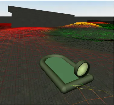
Figure 4: Water Geometry. The red value represents the water’s height.

The normal map is an image in which each pixel represents a direction, namely, the direction

of the water’s surface on a given point. The normal map can be combined with other normal

maps or with normals associated with the geometry’s vertices so as to make the water appear

more animated and believable. The method used in our implementation of water rendering

used normal maps generated through Perlin Noise [11]. Perlin Noise, invented in 1985 by

Ken Perlin, uses several layers, or octaves, of randomly generated noise. Each octave

contains noise at half the frequency of the previous octave. When the several octaves are

resulting texture is similar to a fractal in that it has a definite—but still random—form to it.

Our normal maps were created from a height field generated by Perlin Noise techniques.

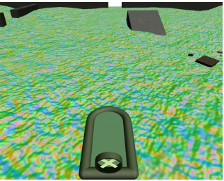
The rendered water with a normal map projected onto it can be seen in figure 5.

Figure 5: Normal Mapping

Reflection and refraction maps are where the bulk of the water’s color comes from. These

maps are usually rendered at the beginning of a frame. The reflection map consists only of

objects that lie above the water normally, but are reflected across the geometry to appear to

lie below the water’s surface, similar to how a reflection of one’s face appears to originate

underwater. It is also possible to use a cube map—a textured cube which, when viewed from

the inside, provides a 360° x 180° field of view of the environment from a particle

location--for reflections, which can be rendered once at the start of the program. This technique

produces very believable reflections, but breaks down if objects are close to the water, as

13

principle to the reflection map, but is much easier to generate. This map represents light

from objects that can be seen below the water’s surface. No geometry transformations need

occur, so all geometry below the water’s surface is simply rendered and saved to a texture

map. Without a refraction map, water will look less believable as it will not distort the

appearance of objects lying below it.

High dynamic range (HDR) rendering techniques are also useful to reflection and refraction

rendering. HDR rendering is a method of storing color that is capable of handling values

greater than 1.0 for the red, green blue, and alpha channels. When objects in a scene are

much brighter than other objects (such as the blue sky compared to shadows), HDR

rendering allows the storage of large color values without clamping them to white, as the

standard OpenGL pipeline does. This lets the sun and other bright objects in the scene show

through in reflections and refractions, even when only a small percentage of the incoming

light is reflected or refracted.

The shader program is where the magic of water rendering occurs. A shader program

consists of specific blocks of code to specify the exact way in which each vertex and pixel of

the water’s geometry are rendered to the screen. As seen in Figure 6, the vertex and pixel, or

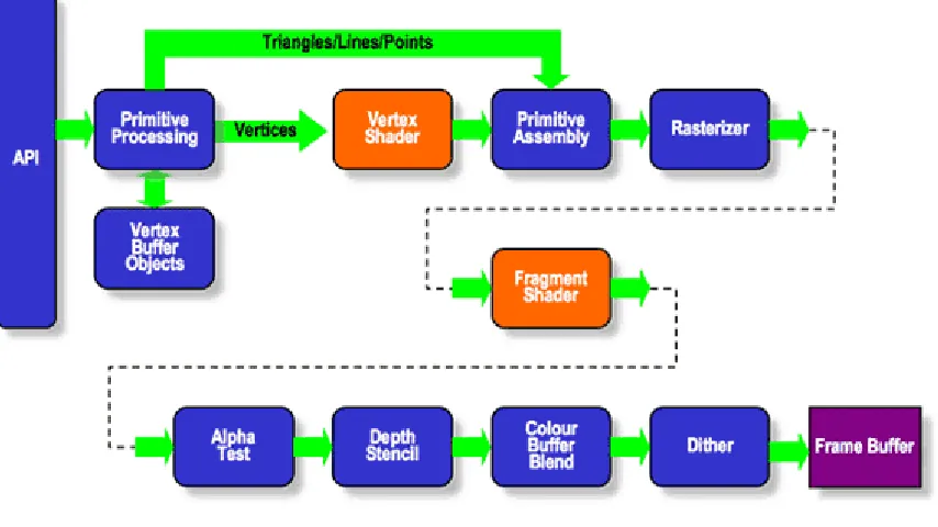
fragment, shaders replace important parts of the OpenGL rendering pipeline. The fragment,

shader is the primary engine for combining all of the colors and lighting effects that create

the appearance of water. The shader calculates a surface normal [12], usually coming from a

normal map, and uses this normal to making lighting calculations as well as to determine the

Figure 6. Shader placement in the OpenGL pipeline. (khronos.org)

Other effects that are often used to achieve a higher degree of believability in real-time water

rendering include water murk effects and caustics. The former is the fog that is present in all

water that is not perfectly transparent. It reduces the amount of light that reaches objects

underwater as well as reducing the light that reaches back up through the water’s surface.

Murk is easily approximated using the formula in equation 1 (adapted from OpenGL.org).

Kmurk = e-(f * d) (1)

In this equation, f is the magnitude of the fog and d is the distance between the water’s

surface and the underwater object. Fog is added by mixing its color with the color of the

15

Caustics are the effect of light rays being refracted by the water’s surface before they strike

objects below. The light is concentrated in some areas and dispersed in others, creating a

moving pattern projected onto all underwater objects. Although ray-tracing light rays

through the water’s surface will create caustics, this is not yet a useful solution for real-time

rendering due to the additional computation required. Therefore, many implementations of

caustics currently use an animated, tiled texture projected onto all scene objects from the

light source’s perspective. Real-time implementations of caustics do exist, however, using

refraction calculations across the water’s surface. [26] and [28] describe methods of

generating these caustics.

The final feature of simulated water is its physical interaction with other objects in the scene.

There are two directions in which this interaction occurs: 1) water affecting objects and 2)

objects affecting water. The first of these effects is much easier to simulate than the second.

Because objects can be modeled as rigid bodies in a physics engine, it is simply a matter of

determining the forces on them from water. Previous research, including Reinot [13] and

Fagerlund [21], simulated buoyant objects by approximating their volume with sample

points. Each sample point was then compared to the water level. If the point lay below the

water’s surface, an upward force was applied to the object at that specific point. The

magnitude of the force was equal to the buoyant force from the water on the volume of the

object accounted for by that sample point. Equation 2 shows the buoyant force on an object

Fbuoyant = VdisplacedWater ρwater g (2)

Using this equation, and treating the sample point as a volume that is either underwater or

above water with no in-between state, it is easy to show that the force on an object at each

underwater sample point is as given in equation 3.

!

Fpoint=Vobject"waterg N

(3)

Where N is the number of sample points in the object. The effect of these forces is very

similar to that of actual buoyancy on a real object, and virtual objects floating in the water

will bob up and down in a believable manner.

The effect of objects on water is more difficult to simulate. The two most common ways of

showing water reacting to things in it are particle systems and simple physical simulation. A

particle system, in the broad sense, is a group of objects with similar behaviors that are

created and destroyed in response to events in the program. Common examples of particle

systems include sparks, smoke, and footprints. [14] When used in water rendering situations,

particles generally consider of drops of water or small ripples on the water’s surface. These

are created in response to events that trigger splashes and other disturbances, such as an

17

Chapter 3

Method Development

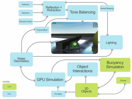
Figure 7 shows the different components needed to create the final rendered water. The

unique features developed in this research will be discussed in the following sections.

Figure 7: Flowchart of the simulation and rendering process

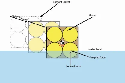
Buoyancy

Buoyant force is the force of displaced fluid pushing up on a submerged object. It is equal to

the weight of the displaced fluid. In this thesis the term buoyancy is expanded to describe the

relatively easy to integrate with a physics engine. Based on the work of Reinot, a buoyancy

model of each physically simulated object was created by approximating its volume with a

set of spheres called “floaters.” A floater can be thought of as a particle that represents a

portion of an object’s total volume and is the intermediary between the water dynamics and

the rigid body physics. The object’s volume is divided equally among the floaters distributed

throughout it, and those floaters are attached to the object’s physical body by a fixed offset

vector. At each timestep of the physics engine, the heights of the floaters relative to the

water are calculated, and from that the portion of each floater that is submerged and being

affected by the water is computed.

In addition to the buoyant force of the displaced water, the water’s motion relative to an

object exerts a force on the object. The equations describing this force are too complex to be

handled in real-time, but a reasonable substitute can be found in the following equation [21].

!

Fdrag =

CdragV 2

A

2

(4)

One thing to note is that the direction of the relative water motion is not accounted for in this

equation. It is easily understood why a boat is more apt to move forward than sideways in

water, but it is not so easy to explain this to a computer and have the simulation account

properly for it. To do so would require fluid simulations of the physical object and would be

very difficult to formulate, so a simplified method is used. Each floater optionally contains a

19

calculated, the relative water motion along this axis is partially or fully removed from the

total velocity. Equation 5 shows the method for accomplishing this.

!

v=v+n ˆ _slip(n_slip •v)

when (nslip • v) < 0 and |v| ≤ 1.0

(5)

After the relative water motion and buoyant forces are calculated, each floater applies its

force to the simulated physical body to which it is attached. Each force is applied to the

floater’s attachment point so the correct moments are also applied. Figure 8 shows a diagram

of the forces exerted by the floater on the object to which it is attached. For simplification, a

slip axis is not shown on the object, but it is easy to see how the floaters affect the object in

ways similar to the way a real fluid would.

Displacement Simulation

A more difficult problem in water modeling is the dynamics of the water itself and the effect

that moving bodies have on the water. Various methods of calculating fluid dynamics exist,

but the technology is computationally expensive and cannot currently run in real-time.

Two different methods for water dynamics were examined: 1) water column diffusion, and

2) particle-based disturbances. The first method is a type of simplified physical simulation,

where a rectangular or hexagonal grid of “water columns” [9] is treated as a set of

interconnected masses moving vertically on damped springs. The second method avoids the

processing overhead of physical simulation and instead harnesses the graphics processor

(GPU) to convert a system of particles into a water height map. It should be noted that these

two methods were used separately, although using them simultaneously is mentioned as part

of future work.

Water Column Diffusion

In this method, the water’s surface is divided into a regular grid. Each point on the grid, or

node, can move along its vertical axis and is attracted to each of its eight adjacent (horizontal,

vertical, and diagonal neighbors) nodes, as well as to its “home” position (usually a

displacement of zero). The attraction force is weighted by the proximity of the neighboring

squares, with the diagonal neighbors exerting less force on a particular point than its direct

neighbors. In addition to this spring-like force, a damping force, proportional to the node’s

21

point on the grid hundreds of times per second, where Ks is the spring constant and Kd is the

damping constant.

!

fnode =("orthogonalNeighbors+

2

2 "diagonalNeighbors#ynode)Ks#Kdvnode (6)

Once new positions and velocities for the node are calculated, a smoothing effect, in which

the node’s height is linearly interpolated between the heights of its eight neighboring nodes,

weighted in the same matter as the force propagation, is applied to it. The new position of

node after a simulation step is y3, given by:

!

y₁=y₀+v₀dt+ f_nodedt2

y₂=(1"0.707C_smoothingdt)y₁+0.1768C_smoothingdt(#diagonalNeighbors)

y3=(1"Csmoothingdt)y21+0.25Csmoothingdt(#adjacentNeighbors)

(7.a)

(7.b)

(7.c)

Where the smoothing factor Csmoothing is on the order of 0.001.

This network of springs can provide a convincing simulation of a fluid surface, with waves

spreading, combining, and propagating. For added reality, certain nodes, such as those along

the edge of the water body as well as those directly underneath large, immoveable objects in

the water, are held in place, or pinned, with a position and velocity that always stay at zero.

These pinned nodes act as hard boundaries on the water’s surface, and can reflect and refract

the water’s waves. Finally, methods having objects interact with this mesh-based water

potentially interact with the water were drawn onto an “interaction image”, with the color

channels representing the minimum and maximum heights of the object at that particular

point, as well as the speed of that object. The resulting image was similar to a two-sided

height map, with extra data embedded in it, representing the speed of the moving objects.

This information was used to force water downward when the object moved through it, as

well as raise it upward in areas immediately in front of a the moving object.

When all of these features were added together, the water column diffusion method provided

for highly believable water interaction as will be shown in examples in the next chapter. The

fluid behaves in a believable manner and interactions occur easily with objects in and around

the water. However, simulating such a mesh in real-time requires a great deal of processing

power. On modern processors, such as the Intel Core 2 Duo, the necessary calculations for a

water grid with 256 x 256 vertices can only run at around 4.75 frames per second.

It’s simply not feasible to simulate water of reasonable resolution in real time on the CPU

alone. Fortunately, the calculations for simulating mesh-based water are very parallel in

nature. That is, the forces on any given node in the mesh can be computed without affecting

the other nodes. This makes water mesh calculation a perfect task for a GPU.

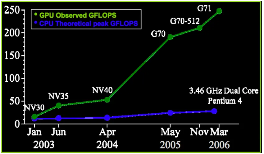
The Graphics Processing Unit, or GPU, on a computer is often much more powerful than its

CPU. But while the CPU is designed to be extremely flexible in the way it handles data and

23

pixels, one by one, at extraordinary speed. Figure 9 shows one comparison of processing

power between recent model GPUs and CPUs.

Figure 9: GPU vs CPU Performance (Courtesy of NVidia)

Because of this design, the GPU is limited in the types of calculations it can perform.

Specifically, it can only write data to one location at a time. However, this limitation is no

problem for water mesh simulation, as only one mesh node at a time is being computed. This

method of harnessing the system’s GPU for non-graphics calculations, called General

Processing on Graphics Processing Unit (GPGPU) has been around for several years, but its

use to supplement CPU calculations in real time situations is relatively rare. NVidia [15] has

done extensive work in this area, integrating the Havok physics engine with their graphics

cards. The results have been very complex, beautifully rendered and physically simulated

Figure 10: GPU-based physics allow for highly complex scenes to run in real-time

Particle-Based Disturbances

The other method of water displacement experimented with was particle-based disturbances.

Under this technique, a system of particles representing disturbances in the water, such as

ripples and v-shaped wakes, is used to deform the water’s surface. The only simulation

required with this method is that of the individual particles, which generally number less than

two hundred, as opposed to thousands of mesh nodes that are calculated using the water

25

pixel represents the height of one vertex of the water’s mesh. Each disturbance is drawn onto

this texture, its color and shape representing the magnitude and way in which it deforms the

water. For example, a ripple disturbance is drawn as an expanding ring onto the water’s

height texture. The height information contained in the final texture is used to draw the

water’s surface, with very effective results.

Disturbances were generated by events such as a virtual boat’s motor being engaged or

objects breaking the water’s surface. Each such event adds a disturbance particle to the

water, which would then update and simulate the disturbance for several seconds. When the

disturbance has damped out, usually by way of an exponential decay function, it is removed

from the simulation, to allow space and processing power for new disturbance particles.

Figure 11 shows disturbance particles in action. The rings represent ripples and waves

caused by objects intersecting the water’s surface, while the straight lines represent the wake

Figure 11: Particle-based Disturbances shown as lines and circles

Rendering

The process of turning a set of texture images and other data into realistic-looking water is a

complex one. For this, extensive use of the reprogrammable nature of current graphics cards

was taken advantage of by creating several vertex and pixel shaders, written in the GLSL

shader programming language. A shader is a program that explicitly directs the GPU on how

to handle the vertices that make up the drawn geometry as well as the pixels that result

27

require the programmer to write code in something resembling compiled assembly code [17],

GLSL language is set up to be very similar to C/C++, which makes writing shaders very

simple and clear.

Shaders make use of several inputs: Vertices, matrices, normal coordinates, texture

coordinates, uniforms, and textures. Vertices, normal coordinates, and texture coordinates

are values explicitly sent to the shader for each point, or vertex, of the rendered geometry.

Matrices affect the size, shape, orientation, and position of the geometry on screen.

Uniforms are values variables fed to the shader before it begins rendering, and are the same

for each vertex rendered. Textures are images used to add realism or special effects to the

scene. In the case of water rendering, textures store images of objects that are reflected or

refracted in the water, as well as height maps and other data used by the shader to make the

water appear believable.

A number of shaders, both simple and complex, were used for this water simulation. The

most basic was called “Float Color.” Its purpose was to allow drawing objects with color

values exceeding 1.0, which is OpenGL’s standard limit on color values. It accomplished

this by simply not clamping the values of the output color to 1.0. Storing these values is

another issue, which will be addressed later in this thesis.

The next shader used was “Object Shader” and was used for drawing all objects in the scene

except for the water. The Object shader used two texture inputs—main texture and water

part, the Object shader simply replicated the standard OpenGL shading pipeline for a single

texture and light source, albeit with per-pixel light calculations instead of per-vertex.

However, when it was set to reflection or refraction mode, the Object shader performed

per-pixel clipping of geometry, ensuring that reflections and refractions only appeared below the

water’s surface.

The Water Shader

The final, and most complicated shader was the “Water Shader”. Many inputs went into the

Water Shader, including reflection and refraction textures, a refraction depth texture, a

small-scale ripple pattern, and, most importantly, the water’s height map. Much of what the Water

Shader did was fairly standard for water rendering: Combining reflections and refractions

that have been distorted based on the surface direction of the water, weighting them based on

a simplified model of the Fresnel Effect, and computing specular lighting effects. However,

the Water Shader contained features not generally found in other water shaders. The first of

these was on-the-fly normal calculation, in which the surface direction of the water was

calculated at draw time in the shader’s vertex program. Geometry normals are traditionally

calculated using the Newell Method [18 p 292], in which triangles are formed out of adjacent

29

For each triangle with vertices v0, v1, and v2, the normal N can be found by

Nx = (y0 – y1)(z0 + z1) + (y1 – y2)(z1 + z2) + (y2 – y0)(z2 + z0)

Ny = (z0 – z1)(x0 + x1) + (z1 – z2)(x1 + x2) + (z2 – z0)(x2 + x0)

Nz = (x0 – x1)(y0 + y1) + (x1 – x2)(y1 + y2) + (x2 – x0)(y2 + y0)

(8)

The normal at each vertex of the geometry is then estimated by averaging the normal of each

triangle that borders it.

This method is very effective for calculating a smooth surface from a set of arbitrary points,

but it is computationally expensive. In the case of the regular, rectangular grid layout of a

water mesh, a shortcut was used. A small section of the mesh is shown in Figure 12, with

five key points labeled. Normally, the Newell Method would be used to calculate normals

for the triangles ADP, DBP, BCP, and CAP, which would then be averaged to find the vertex

normal at P. If the Newell Method is applied using only variables for coordinate values, the

final value for the normal at P can be found with a much simpler equation:

N = (By – Ay, 2du, Dy – Cy) (9)

Figure 11 shows an example of this calculation. When compared to the Newell Method, the

results were visually and numerically identical, but the frame rate was significantly higher.

The Water Shader takes advantage of this trick by reading vertex height data into the vertex

work to be done on the GPU rather than the CPU. Thus, the vertex texture contains the

dynamic height data to be read in the vertex shader, so display lists can be used to render the

geometry, freeing the CPU to work on other tasks.

Figure 12: Normal Calculation from Neighboring Vertices

Another newly developed feature unique to the Water Shader is excitement mapping.

Excitement mapping simulates, on a per-vertex basis, the amount of small-scale turbulence

present on the water’s surface. This process is analogous to specular mapping of solid

31

change in the amount of highlight and shine on the object. The effect of excitement mapping

is to make water appear more turbulent when it moves rapidly, such as in the case of waves.

This is accomplished by reducing the amount of reflection and highlight for excited areas of

water. Excitement is calculated by estimating the sum of kinetic and potential energy of a

particular water mesh node, as well as by its difference in vertical position and velocity from

that of its neighbors.

The third special feature of the water shader is reflection-refraction tone balancing (RTB), an

operation similar to tone mapping. Tone mapping is a process in which the color values of

an image are balanced to more closely match what the human eye would see in real life.

Welsh [19] used an average luminance model to brighten darker colors while ensuring

brighter colors didn’t become washed out. His formula is shown in equation 9, where

luminance is the average of the red, green, and blue color channels.

Color = color * (1.0 – e^luminance * 8.0) / (luminance) (10)

RTB adds realism and believability to the scene by forcing the image to lean towards either

showing reflections on the water’s surface or refractions beneath it, but not both. This is

similar to how water appears in real life. For example, when standing over a calm lake, you

generally see the reflection of the sky in the water, but if you look downward into your own

reflection, which is much darker than the sky, you will see through the water’s surface and

refracted objects below it become visible. RTB works by using a method similar to tone

found. The refracted light is then brightened or darkened based on the luminance of the

reflected light.

The Render Sequence

The final aspect of rendering water is the render sequence itself. The types of prerenders

done every frame are critical to the final product. For this method the following information

was rendered to textures: Reflections, refractions, refracted object z-depth, water z-depth,

and water height map. Each of these has a key role in the appearance of the water. The

reflection and refraction textures are relatively self-explanatory. Reflections are images of

objects above the water that are reflected in its surface, while refractions are objects under

the water, the light from which is bent as it passes through the water’s surface. For

reflections, the water z-depth texture is used to clip the reflected geometry so that only

objects that lie above the water’s surface are reflected. In the case of refractions, the same

surface clipping can be used, although it isn’t as important because objects above water will

obscure most refractions that appear above the water. When rendering the water, the

refraction z-depth texture is used in conjunction with the refraction texture to determine how

much water is between the user’s eyepoint and the refracted object. This information is used

to add murkiness and cloudiness to the water, obscuring the refracted objects. To determine

33

!

Deye =

"zfarznear

(zfrag"0.5"

zfar+znear 2(zfar"znear)

)(zfar"znear)

(11.a) adapted from [16])

Dunderwater = Deye(object)-Deye(water) (11.b)

Several advanced rendering techniques, available only on very recent graphics cards, were

used to implement the method into a software application. These include floating point

frame buffer objects (FBOs), clipping surfaces, and vertex shader texture reads. Floating

point FBOs are virtual screen buffers that store pixels as 16-bit signed float values with a

practically unlimited range of values, rather than 8-bit unsigned chars that can only store

values from 0-1. This allows the physics of water to be simulated on the GPU with enough

precision to produce stable and consistent results. Floating point FBOs also allow negative

values to be stored as well as values greater than one, enabling data other than color to be in a

texture, as well as HDR color for storing values.

Clipping surfaces are another innovative aspect of the application. Regular clipping methods

only allow clipping against a flat plane. Clipping surfaces use 24-bit depth buffer values

stored to a texture to discard geometry (per pixel) that is either farther from or closer to the

camera than the clipping surface. In this water simulation, clipping surfaces are used to limit

reflections only to objects that lie above the water’s surface. Because the water’s surface

moves and deforms, a regular clipping plane would be of little use for clipping the geometry,

buffer generates the clipping surface used in the simulation. The resulting depth data is

compared to the rendered refractions and reflections, with pixels of the rendered objects

being discarded if they are closer to the camera than the water’s surface.

Finally, the last advanced graphics technique is vertex shader texture reads. Although it has

been in the OpenGL specification for several years, it is only recently that graphics hardware

has begun to support reading from textures in a vertex shader. By using vertex shader texture

reads, height map data for the water can be read for each vertex, as well as the surrounding

vertices, enabling the on-the-fly normal calculations mentioned earlier. When vertex shader

texture reads are used to calculate this information, all of the dynamic information needed to

render the water is stored in its textures, allowing a display list to be used to render the

water’s geometry. Compared to immediate mode rendering, in which the CPU sends

35

Chapter 4

Results and Discussion

Several measures of performance are used to test the two main water simulation methods.

The most basic method is simply looking at the graphical frame rate achieved by the

program. Another method useful only for the physically simulated water is the “Simulation

Time Ratio.” This number represents the number of seconds of physical simulation that can

be calculated in one second of real time. Next, the most valuable benchmark is simply that

of visual appeal. The overall smoothness of the program and believability of the water’s

surface is the real goal for this research, and can therefore be used as means of evaluation.

These factors were all judged for the various modes of water, both with and without vertex

shader texture reads (“GPU Geometry”). Finally, QuickProf [20] profiling software was

used to determine performance benchmarks of the simulation and find what parts of it were

taking up the most time. Bottlenecks were identified and will be discussed. The results are

tabulated below, with results in parentheses indicating GPU geometry is turned off.

Table 1: Frame Rate

Water Mesh Size (vertices)

Particle Water (fps) CPU Mesh Water (fps) GPU Mesh Water (fps)

64 x 64 29(29) 34(26) 29(26)

128 x 128 29(28) 2(2) 29(20)

256 x 256 29(16) 0.34(0.36) 20(15)

512 x 512 29(6) 0.09(0.09) 6.6(3.3)

It can be clearly seen from table 1 that CPU mesh water slows down drastically for higher

calculations required being proportional to the square of the mesh size. When GPU

geometry is turned on, mesh size has little effect on both the particle water and the GPU

mesh water except at the highest mesh size tested. In the case of particle water, this is

because no per-vertex calculations are performed on the water. Although per-vertex

calculations are used for the GPU mesh water, the speed at which the GPU can process the

vertices is so great that, for the most part, it is relatively small in comparison to the other

graphics operations required for GPU simulation, and thus mesh size has a much smaller

effect on the frame rate than it does for the CPU simulated water.

The next chart shows the change in Simulation Time Ratio (STR) for different water

simulations. Particle water is left out of this comparison because it is not actually simulated,

so the STR is undefined. Note that a simulation time ratio of 1.0 is the minimum value at

which the simulation can continue to run in real-time, assuming zero overhead for all the

other program functions, such as rigid body physics and rendering.

Table 2: Simulation Time Ratio

Water Mesh Size CPU Mesh Water GPU Mesh Water

64 x 64 2.1 21

128 x 128 0.19 21

256 x 256 0.09 22

37

The results of this test are striking. The CPU-based water degrades in performance very

quickly. At a mesh size of just 128 x 128, its STR is far below the minimum necessary value

of 1.0. It is worth nothing that the 128x128 node water grid performs less than 10% as

quickly as the grid with one-fourth the number of nodes. This indicates that the speed of the

CPU-based simulation is dependant on more than simply the number of nodes. It is likely

that the cache and data bus of the computer limit the flow of data significantly. The

GPU-based water, on the other hand, showed no performance decrease at all with increasing the

number of nodes (pixels) simulated.

The next evaluation is purely subjective. It examines the believability and smoothness of the

water simulation visually. The primary comparison made here is particle-based water versus

simulated mesh water. Figures 13-18 are images of simulated water demonstrating all the

Figure 13: Particle-based Water (note the ripples caused by floating objects)

39

Figure 15: Particle-based Water (note the light reflection off the surface as well as the objects under the water)

Figure 17: Waves moving across the surface of GPU-based water

41

The particle-based water has nice-looking responses to splashes and other interactions with

the water, thanks to the splash detection system. Ripples and waves move quickly and

believably across its surface, but no medium-to-long term turbulence in the water results for

the particle-based interaction. Additionally, waves are not reflected or refracted by stationary

objects, such as walls, in the water. In terms of speed, however, when GPU geometry is

used, the water runs smoothly at all resolutions tested. Overall, the water looks good, but its

interaction modes are very limited.

Mesh-based water is far more interactive than particle-based water. By using images for

interaction, any object touching the water can affect its motion, based on the object’s velocity

and position. Once interaction occurs with the water, the water will remain in motion, waves

and ripples bouncing around realistically, until damping forces smooth it out again. When

several objects interact with the water, the resulting effects are very believable and provide

for an extremely effective simulation. Simulating the water on the GPU allows for a fast

frame rate, filling a primary requirement for effective water rendering. Mesh-based water is

not without its drawbacks, though. The methods used for pushing the water up and down

tend to cause erratic behavior in slow moving objects. In an effort to cause stationary or very

slow-moving objects to have little effect on the water around them, while faster-moving

objects cause waves and ripples, the behavior of the water tends to change rather abruptly

when an object at rest is put into motion. Overall, however, the mesh-based water provides

for a much more believable experience than the particle-based water. The results of other

effects are also visible in the figures. Figures 13 and 15 show objects both above and below

more visible, similar to the way in which our eyes adjust to light levels depending on where

we look. The refraction of the objects by the water is also visible in these images.

Performance Bottlenecks

By using the Quickprof performance profiling software, it was determined where the

computer was spending the most time for each of the three rendering modes. Figure 19

provides a charts breaking down the performance of each mode, based on specific tasks

required for that simulation method.

Figure 19: Processing Time Breakdown

In both the particle and GPU-based water, the main bottleneck was the transfer of the water

data texture from the GPU to the main memory. While this data transfer is necessary for the

program to behave properly, it could be reduced in frequency. Rather than the texture

43

noticeable effect to the simulation fidelity. Starting from a base frame rate of 30 fps, if the

texture was downloaded every 10 frames, two thirds of the “texture download” piece of the

pie would vanish—almost 37% of the total cycle time for the GPU-simulated water. This

time would likely be used to significantly boost the frame rate, as all non-graphics operations

occur at a constant rate and therefore would not speed up or otherwise expand to take up the

extra available CPU and GPU time.

The other major bottleneck across all three simulation modes is the non-water drawing, of

which a significant part is devoted to creating the various prerendered textures. Optimizing

this part can be accomplished through any number of standard graphics speed-up techniques,

Chapter 5

Summary, Conclusions and Future Work

In this thesis, a method for creating believable, useful water for games and real-time

simulations was presented. Unlike many other demos and simulations, the ideas presented

here are designed to be integrated into an application to enhance it, rather than standing alone

and using all of the available computing power for the water and its simulation. It does this

by taking advantage of the massive resources available on modern GPUs for fast calculations

and minimal CPU usage. Perhaps the best advancement in this thesis was the use of

texture-based interaction, which allowed the GPU-texture-based water simulation to account for objects

moving into, out of, and through the water without costly texture uploads and downloads.

The simulations discussed here are also significant in that they rely on the very latest in

graphics hardware. All simulations ran on an NVidia GeForce 8800 card, which is one of the

first cards to fully support reading from textures in the vertex pipeline.

When these features were used, the GPU-simulated-and-rendered water tremendously

outperformed the CPU-based water at all mesh sizes larger than 64 x 64 nodes. Overall, the

particle disturbance-based water has the fastest performance, but it generally fell short in

terms of visual quality and believability.

There is a great deal of options for future work on this topic. One obvious path to pursue is

the drawing of real-time caustics [24, 28]. Another future goal is the simulation, with particle

45

GPU-based water with both particle system-based and image-based object interaction

techniques could encompass a wider range of small- and large-scale detail. Finally, another

possible goal is the combination of procedurally generated water, such as that described in

the Typhoon engine and [28], with the simulated water methods described in this thesis.

References

1. Tyson, J. “How Industrial Light & Magic Works.” Retrieved March 2007, from http://entertainment.howstuffworks.com/perfect-storm.htm.

2. Warzecha, N, Spille-Kohoff, A. (2006). Fluid Motion. Mechanical Engineering. September 2006.

3. National Aeronautics and Space Administration. “The Blue, the Bluer, and the Bluest Ocean.” Retrieved April 2007 from

http://daac.gsfc.nasa.gov/oceancolor/scifocus/oceanColor/oceanblue.shtml 4. Floor, A. (2000) “Oceanography: Waves.” Retrieved April 2007 from

http://www.seafriends.org.nz/oceano/waves.htm.

5. Kipfer, P. and Westermann, R. 2006. Realistic and interactive simulation of rivers. In Proceedings of Graphics interface 2006 (Quebec, Canada, June 07 - 09, 2006). ACM International Conference Proceeding Series, vol. 137. Canadian Information

Processing Society, Toronto, Ont., Canada, 41-48.

6. Enright, D., Marschner, S., and Fedkiw, R. 2002. Animation and rendering of

complex water surfaces. In Proceedings of the 29th Annual Conference on Computer Graphics and interactive Techniques (San Antonio, Texas, July 23 - 26, 2002). SIGGRAPH '02. ACM Press, New York, NY, 736-744. DOI=

http://doi.acm.org/10.1145/566570.566645

7. Rademacher, P. “Ray Tracing: Graphics for the Masses.” Retrieved April 2007 from http://www.cs.unc.edu/~rademach/xroads-RT/RTarticle.html.

8. Waters, Z. “Photon Mapping.” Retrieved May 2007 from

http://web.cs.wpi.edu/~emmanuel/courses/cs563/write_ups/zackw/photon_mapping/P hotonMapping.html.

9. DiFranco, D., Fu, L., Ju, P., & Rikert, T. (1997). “Physics-Based Fluid Model for Haptic Interaction.” (MIT Graphics Class Project)

10.Zelsnack, J. (2003) “GPU Water Simulation.” Presented at Game Developer’s Conference ‘03.

11.Elias, H. “Perlin Noise.” Retrieved November 2006 from http://freespace.virgin.net/hugo.elias/models/m_perlin.htm.

12.Humphrey, B. (2005). "Realistic Water Using Bump Mapping and Refraction." Retrieved June 2006, from http://www.gametutorials.com/gtstore/pc-319-1-heightmap-6-realistic-water-using-bump-mapping.aspx.

13.Reinot, A. “Andres’s Computer Graphics Blog (November 11, 2005 Entry).” Retrieved 6-19-2006, from http://reinot.blogspot.com

14.Hammersly, T. (2004). “Particle Systems.” Retrieved March 2007 from http://www.devmaster.net/articles/particle_systems/.

15.Green, S. Harris, M. “Havok FX Physics on NVidia GPUs”. Presented at Game Developer’s Conference ‘06.

16.“OpenGL Reference Pages.” Retrieved March 2007 from http://www.opengl.org/sdk/docs/man/

47

18.Hill, F. (2003). “Computer Graphics Using OpenGL: Second Edition.” Prentice Hall.

19.Conversations with Terry Welsh regarding water and vegetation rendering. 2006-7. 20.Streeter, T.. “Quickprof Project Website”. Retrieved March 2007 from

http://quickprof.sourceforge.net.

21.Fagerlund, M. "Buoyancy Particles or Bobbies." Retrieved May 2007, from http://www.hypeskeptic.com/Mattias/DelphiODE/BuoyancyParticles.asp. 22.Hart, E. (2007). "GPU Christmas Tree Rendering." Retrieved March 2007 from

http://developer.download.nvidia.com/SDK/10/opengl/src/xmas_tree/doc/GPU_Chris tmasTree_Rendering.pdf

23.Lionel E., Décoret, X. (2006). "Realistic Water Volumes in Real-Time." Proceedings of the Eurographics Workshop on Natural Phenomena ‘06: 1-8.

24.Loviscach, J. (2003). "Complex Water Effects at Interactive Frame Rates." 25.Rost, R. (2005) “Introduction to the OpenGL Shading Language.” Developer

Presentation. Retrieved May 2007 from

http://developer.3dlabs.com/documents/index.htm.

26.Stam, J. (2003). "Real-Time Fluid Dynamics for Games." Presented at Game Developer’s Conference ‘03.

27.Lanza, S. (2005). “Animation and Display of Water”, SHADERX3: Advanced Rendering with DirectX and OpenGL. Charles River Media, Inc.

28.Jensen, L. (2001) “Deep-Water Animation and Rendering,” Gamasutra,

http://www.gamasutra.com/gdce/jensen/jensen_01.htm

Acknowledgements

I’d like to thank the following people for their support in getting me to where I am today.

•My parents, for, well, everything. I don’t know where I’d be without them.

•Dr. Adrian Sannier, for seeing potential in me and giving me guidance in my life when I needed it more than I ever had, but didn’t realize it. Without him, I wouldn’t be in grad school right now.

•Dr. Eliot Winer, for having faith in me and supporting me even when I was starting to veer off the engineering course, and for recognizing that another path might be better for me.

•Andres Reinot, for helping me to become an OpenGL guru of sorts, as well as offering me plenty of artistic and programming advice.

•Kevin Teske, partly for his role in keeping the VRAC computers up and running, but mostly for being a mentor and counselor to me whenever I needed advice, encouragement, or just an honest opinion on my latest graphics work.

•Tyler Streeter, for his help with the physics engine and program debugging.

•Ted Martens, for a great deal of artistic input.