Optimized Controller Design by Real Time Model Identification

(1)

International Journal of Innovative Technology and Exploring Engineering (IJITEE) ISSN: 2278-3075, Volume-8 Issue-8S2, June 2019



Abstract: Most of the processes with various dynamic characteristics can be reduced to the SOPTD model by using the model reduction method. In this paper, we use the control structure with the Smith predictor to compensate the delay time of the SOPTD model to minimize the ITAE The control algorithm is used. We also propose an optimally adaptive PID controller design algorithm that estimates the coefficients of the SOPTD model in the Smith-Predictor control structure and changes the PID controller parameter values. The method of obtaining the reduced model is improved by using numerical calculation and genetic algorithm. As a result, the steady - state response of the higher - order model and the reduced model is perfectly matched for the unit feedback input. In the optimization adaptive PID controller design, the control parameter value is obtained so that the performance index ITAE is minimized in the Smith Predictor control structure using the reduced model, and the RLSE is used to obtain satisfactory control performance when the external influence is large We propose an adaptive PID controller algorithm that estimates the coefficients of the SOPTD model in real time and then changes the PID controller parameter values from the estimated coefficients by applying the previous method. Simulation results show that the proposed adaptive control scheme has good adaptability to disturbance and process variations.

Index Terms: Model Reduction, Adaptive control, Smith predictor, PID Control.

I. INTRODUCTION

Proportional and Integral and Derivative (PID) controllers are widely used in the process industry because they are easy to understand, simple in structure and easy to implement[1-4]. The most important thing when designing a PID controller is to determine the parameter. Therefore, many researches have been made on the method of determining the parameters of the PID controller [5]. Among them, Ziegler-Nichols Rule, Cohen-Coon Method, IAE, ISE, ITAE and IMC methods are widely used. However, most of these methods are easy to apply for primary and secondary models, but are not easily applicable for higher order models. Therefore, research is being conducted on a tuning method of a general - purpose PID controller that can obtain good performance for a high - order model or a process with a large delay time. Recently, there is a method to directly obtain the control parameter value by using the coefficient value of the reduced model[6-8]. In parallel with this universal controller design method, it is necessary to obtain a reduced model close to the actual model. The research on the reduction model is performed in the time domain and the frequency

Revised Manuscript Received on May 23, 2019.

Hyung-Soo Hwang, Department of Electronics Convergence Engineering, Wonkwang University / Iksan city, Jeonbuk, Republic of korea

Joon-Ho Cho, Department of Electronics Convergence Engineering, Wonkwang University / Iksan city, Jeonbuk, Republic of korea

domain and has achieved many achievements. Comparing the model reduction in the time domain with the model reduction in the frequency domain, the reduced model obtained in the time domain is comparable to the response of the real model in the time domain, but not in the real domain in the frequency domain. The model reduction method in the frequency domain is more complex than the model reduction method in the time domain, but it shows that the reduced model is comparable to the response of the real model in both time domain and frequency domain. In the time domain, typical model reduction methods include Pade approximation and Routh stability approximation. Wang's model reduction method is a typical method in the frequency domain[9 -12]. However, Wang's method can’t be applied when the real model does not pass the entire region of the Nyquist line, and there is a case where the steady-state response between the high-order model and the reduced model is inconsistent in the model reduction process. In order to solve this problem, reference points add specific points of the Nyquist diagram to consider the steady state and transient state of the unit feedback input and use the descending descent method and the genetic algorithm to reduce the model Respectively. However, this method also uses the slope descent method to obtain the coefficients of the reduced model, so that the steady state output values for the unit feedback input do not perfectly match. To solve these problems, numerical computation and genetic algorithm were used to obtain the coefficients of the reduced model. In addition, as a controller design method, a real-time estimator using a recursive least squares estimator (RLSE) is added to the Smith Predictor control structure to estimate a coefficient of the SOPTD model in real time when it is greatly influenced by the outside. We propose an adaptive PID structure that changes the values. This paper consists of optimization PID controller design, optimization adaptive PID controller design, simulation and review, and conclusion of Smith Predictor structure.

II. METHODLOGY

Optimized PID controller design with Smith predictor structure

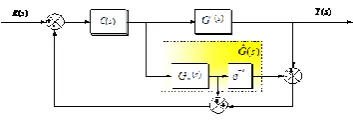
Most of the processes with various dynamic characteristics can be reduced to the SOPTD model by using the model reduction method. In this paper, we use the control structure with the Smith predictor to compensate the delay time of the SOPTD model to minimize the ITAE The control algorithm is proposed. First, Smith predictor control structure, which is well known as a method to compensate the delay time, is adopted. The block diagram is shown in figure 1.

Optimized Controller Design by

Real-Time Model Identification

(2)

[image:2.595.86.263.49.109.2]

Figure 1. Block diagram of Smith Predictor

The closed loop transfer function of the system using the Smith predictor is given by Eq. (1).

𝑌 𝑠 𝑅 𝑠 =

𝐶 𝑠 𝐺 𝑠

1+𝐶 𝑠 𝐺_𝑚 𝑠 𝐺 𝑠 −𝐺𝑚 𝑠 𝑒−𝑠𝐿

(1)

Here, G (s) denotes the actual process, and the formula (𝐺𝑚 𝑠 𝑒−𝑠𝐿) denotes the reduced model. In the above structure, assuming that the actual process and the reduced model are almost identical, equation (1) approximates to equation (2).

𝐺𝑚(𝑠)𝑒−𝐿𝑠 𝑌(𝑠)_𝑅(𝑠)≈

𝐶(𝑠)𝐺(𝑠)

1+𝐶(𝑠)𝐺𝑚(𝑠) (2)

In equation (2), it can be seen that the time delay term of the characteristic equation has been removed. The controller is a PID controller and can be expressed as Equation (3).

C s = k𝐴𝑠2+𝐵𝑠+𝐶_𝑠 (3)

Here, A = 𝐾𝐷 , 𝐵 = 𝐾𝑘 𝑃 , 𝐶 = 𝐾𝑘 𝐼 𝑘

If the parameter value of the PID controller is to cancel the pole of one of the reduced model loop transfer function, that is, A = a, B = If set as b, and c = C Equation (1) is approximated as equation (4). Where a, b, and c are coefficients of the reduced model.

𝑌(𝑠)

𝑅(𝑠)≈ 𝑘 𝑒−𝑠𝐿

𝑠+𝑘 (4)

The Peru transfer function of the Smith Predictor structure in Figure 1 shows that the reduced model is accurate and can be represented as a first-order delay model using a PID controller, and the performance of the closed-loop response depends only on the value of k have. In other words, the optimization problem can be solved by finding the k value with the optimum performance. Genetic algorithms have a disadvantage in that trial and error of setting initial values must be made and execution time is consumed. In this paper, we propose a mathematical analysis of the closed - loop response in the time domain to find the optimal k value. If the input is a unit step function and the set value is 𝑦𝑟, the inverse Laplace transform of equation (4) to equation (5).

y t = 𝑦𝑟(1 − 𝑒−𝑘 𝑡−𝐿 ) (5) In equation (5), the closed loop response characteristic of the system using the Smith predictor is determined by k. By choosing ITAE as a performance index, a k value that minimizes the performance index can be found analytically. From equation (5) the error function is the equation (6).

e t = 𝑦𝑟𝑒−𝑘(𝑡−𝐿), 𝑘 > 0 (6)

The performance index ITAE is expressed by the equation (7) by definition.

ITAE = 𝑡𝑒 𝑡 𝑑𝑡 =𝑦𝑟

𝑘2𝑒

𝑘𝐿 ∞

0 (7)

Since 𝑦𝑟 and L is a constant in the equation (7) can be derived ITAE the k value to the minimum ITAE to be a function only k, through the differential. By differentiating the equation (7), the equation (8) is obtained.

𝑑𝐼𝑇𝐴𝐸

𝑑𝑘 = 𝑦𝑟(𝐿 − 2

𝑘) 𝑒𝑘𝐿

𝑘2 (8)

The ITAE value is minimum is equal to the equation (9).

k =2

𝐿 (9)

In conclusion, the optimal control parameter values of the PID controller in the Smith Predictor structure of Figure 1 are directly derived from the coefficients of the reduced model.

𝐾𝑃 𝐾𝐼 𝐾𝐷

=2 𝐿

𝑏 𝑐 𝑎

(10)

Optimized Adaptive PID Controller Design

The optimization algorithm obtained by using the reduced model described in the previous section compensates for the delay time, but satisfactory control performance can’t be obtained when the influence is externally influenced. Therefore, in order to compensate for these drawbacks, the adaptive controller is required to change the control parameter values appropriately according to external influences. That is, it is necessary to obtain the parameter value of the reduction model in real time and change the control parameter value using Equation (9), so that the performance index ITAE value can be minimized. In this paper, we use the Recursive Least Squares Estimator (RLSE) to estimate the second-order model in real time and add this real-time estimator to the Smith-Predictor control structure in Fig. We propose an adaptive PID controller design algorithm that estimates the coefficients of the SOPTD model and changes the parameter values of the PID controller.

Implementation of real-time second-order system estimator using RLSE

(3)

Second order system of continuous time system can be obtained by converting the obtained differential equation into discrete time state equation, converting discrete time state equation into continuous time state equation and converting it into transfer function. The system to be obtained from the response of the process is the secondary system of Eq. (11).

𝑌(𝑠) 𝑈(𝑠)=

1

𝑎𝑠2_{+𝑏𝑠+𝑐} (11)

Equation (11) can be transformed into the differential equation form of equation (12) by the trapezoidal method.

y kT = 𝑏0𝑢 𝑘𝑇 + 𝑏1𝑢 𝑘𝑇 − 𝑇 + 𝑏2𝑢 𝑘𝑇 − 2𝑇 (12)

here, −𝑎1𝑦 𝑘𝑇 − 𝑇 − 𝑎2𝑦(𝑘𝑇 − 2𝑇), 𝑏0= 𝑇2

4𝑎+2𝑏𝑇+𝑐𝑇2,

𝑏1= 2𝑇2

4𝑎+2𝑏𝑇+𝑐𝑇2,𝑏2= 𝑇2 4𝑎+2𝑏𝑇+𝑐𝑇2,

𝑎1 =

(2𝑐𝑇2−8𝑎) (4𝑎+2𝑏𝑇+𝑐𝑇2₎, 𝑎2 =

4𝑎−2𝑏𝑇+𝑐𝑇2 (4𝑎+2𝑏𝑇+𝑐𝑇2₎

Given the sampling data for an arbitrary process, the coefficients of the differential equation with the form of equation (12) can be found using the LSE

When the model is defined as equation (13), it is substantially the same as equation (12) with the sampling time removed, and the coefficient of the model can be obtained by LSE.

y k = 𝑏0𝑢 𝑘 + 𝑏1𝑢 𝑘 − 1 + 𝑏2𝑢 𝑘 − 2 −

𝑎1𝑦 𝑘 − 1 − 𝑎2𝑦(𝑘 − 2) (13)

∅𝑇_{𝑖 = 𝑢 𝑘 𝑢 𝑘 − 1 𝑢 𝑘 − 2 𝑦 𝑘 − 1 𝑦(𝑘 − 2)}_,

𝜃0_{= 𝑏}

0𝑏1𝑏2𝑎1𝑎2 𝑇

When the model of equation (13) is defined, variables are constructed as in equation (14) using sampling data.

Y t = 𝑦 1 𝑦 2 ⋯ 𝑌 𝑡 𝑇_{, Φ t =} ∅𝑇₍₁₎

⋮ ∅𝑇_(𝑡)

P t = (Φ𝑇_(t)Φ(t))−1 ₌𝑡 _∅(𝑖)∅𝑇_(𝑖)

𝑖=1 −1 (14)

If the variable in equation (14) is constructed, the coefficient in equation (13) can be obtained using equation (15).

𝜃 = (Φ𝑇_Φ)−1_Φ𝑇_{𝑌 = 𝑃}−1_(𝑡)∅𝑇_{𝑌 (15)} When the coefficients of equation (12) are obtained from the input and output data of the process using equations (13) to (15) using LSE, it is necessary to convert to the continuous time second order system. .

The differential equation of Eq. (12) can be transformed into a discrete time state equation as Eq. (16).

𝑥 k + 1 = A𝑥 𝑘 + 𝐵𝑢(𝑘)y k = Cx k + Du(k) (16)

here, A = _−𝑎0 1

2 −𝑎1 , B = 0 1 ,

𝐶 = 𝑏2− 𝑎2𝑏0 𝑏1− 𝑎1𝑏0 , 𝐷 = 𝑏0 The discrete-time state equation of Eq. (16) can be expressed as a continuous-time state equation as Eq. (17).

𝑥 𝑡 = 𝐴 𝑥 𝑡 + 𝐵 𝑢 𝑡 y t = 𝐶 𝑥 𝑡 + 𝐷 𝑥 𝑡 (17)

here, 𝐴 =1

𝑇log 𝐴 , 𝐵 = 𝐴 𝐴 − 𝐼

−1_{𝐵, 𝐶 = 𝐶, 𝐷}_{= 𝐷}

The continuous-time state equation of Eq. (17) can be

expressed as Eq. (18)

𝑑

𝑑𝑡𝑥1 𝑡 𝑑 𝑑𝑡𝑥2 𝑡

= ₋0𝑐 1

𝑎 −

𝑏 𝑎

𝑥1 𝑡 𝑥2 𝑡

+ 01 𝑎

u t (18)

y = 1 0 𝑥_𝑥1(𝑡) 2(𝑡)

+ 0 u(t)

Equation (18) is transformed into a quadratic transfer function as in (19).

𝑌(𝑠)

𝑈(𝑠)=

𝑑𝑠2+𝑥1𝑠+𝑥2

𝑠2_{− 𝑎}₁₁_+𝑎₂₂_𝑠−𝑎₁₂_𝑎₂₁ (19)

here, 𝑥1= (𝑏1𝑐1+ 𝑏2𝑐2− 𝑎11𝑑 − 𝑎22𝑑), 𝑥2=

(−𝑏1𝑐1𝑎22+ 𝑏1𝑐2𝑎21+ 𝑏2𝑐1𝑎12− 𝑏2𝑐2𝑎11− 𝑎12𝑎21𝑑) Using the LSE, the value obtained from the secondary system from the input / output data is used as the initial value of the RLSE, and the parameter value can be obtained by the equation (20) in real time.

𝜃 𝑡 = 𝜃 𝑡 − 1 + 𝐾 𝑡 𝑦 𝑡 − ∅𝑇_{𝑡 𝜃 𝑡 − 1 (20)} K t = P(t − 1)∅(t)(I + ∅𝑇_{(t)P(t − 1)∅(t))}−1

𝑃 𝑡 = (𝐼 − 𝐾(𝑡)∅𝑇(𝑡))𝑃(𝑡 − 1)

Using the reduced model and real-time estimator Optimized Adaptive PID Controller Design

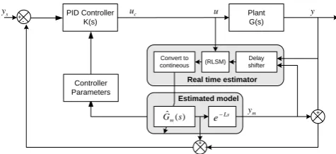
[image:3.595.312.550.476.585.2]

In this paper, we propose a new adaptive PID control algorithm that estimates the coefficients of the SOPTD model in real time when the influence is greatly influenced from the outside by adding it to the Smith-Predictor control structure and changes the PID controller parameter value from the estimated coefficients The controller is implemented. Figure 2 shows the proposed adaptive control algorithm.

Figure 2. Structure of proposed optimized adaptive PID control As can be seen in Figure 2, the model is SOPTD, but the estimator requires a second-order system. Therefore, it is possible to obtain Gm (s) from the process output delayed by the delay time of the reduction model, and by using this value, the adaptive controller can be implemented by adjusting the control parameter value by the method described in this text. The proposed method can be used as an adaptive controller that is robust to changes in disturbance or process parameters by model estimation in real time, and the optimal parameter of the controller can be optimized, so that an optimal adaptive PID controller can be designed.

PID Controller K(s)

Plant G(s)

Estimated model

Ls

e

(RLSM) Delay

shifter Convert to

contineous

Real time estimator

) (

ˆ s

Gm

+

-+ +

-+

s

y

m

y

c

u u

(4)

III. RESULTSANDDISCUSSION

In this paper, the simulation is performed considering the process used in the reference paper [15], and the control performance of the existing control structure is presented. In this paper, the performance of the proposed control structure only the comparison is presented. Consider a tertiary system with a time delay as in step 1.

Process 1.

G 𝑠 = 1

(𝑠 + 1)(𝑠 + 5)2𝑒 −0.5𝑠

The reduction model for the process 1 can be obtained as in Eq. (21) according to Section 2.

𝐺 𝑠 = 1

7.7756 𝑠2_{+32.6507 𝑠+25}𝑒

−0.6076 𝑠₍₂₁₎

When the reduced model is obtained, the PID controller in the control structure of Figure 1 can be obtained from the coefficients of the reduced model.

𝐶 𝑠 = 26.8683 +20.5725

[image:4.595.347.507.50.103.2]

𝑠 + 6.3985𝑠 (22)

Table 1: Comparison of reduced models for process 1

Error in

frequency domain

Error in

time domain

Steady-state error

Wang's

method 1.8928 0.8646 0.0003

Proposed

method 1.1454 0.0856 0

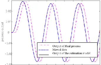
Table 1 shows the error between the real model and the reduced model in the time domain and frequency domain. Where the frequency error is the absolute error for the magnitude in the complex plane, the time domain error is the sum of the absolute errors, and the steady state error is the difference between the steady state output between the real model and the reduced model. As can be seen in Table 1, the proposed method is superior to Wang's method in time domain, frequency domain and steady-state error. If the reduced model and the PID controller are designed, the proposed adaptive control structure can be implemented. The initial parameters of the RLSE can be obtained from the sampling response of the process using the LSE method. The data used in the LSE is the sampling data for the second-order delay system. Since the system to be estimated is the secondary system, Should be moved by the delay time to use the LSE. Figure 3 shows the sine wave response for the actual process, the data shifted by the delay time for model estimation, and the output of the process estimated using the LSE.

The initial parameters are shown in Eq. (23).

P 0 = 102_×

9.7305 9.7263 9.7211 0.1282 0.1260

9.7263 9.7231 9.7389 0.13053

0.1283

9.7211 9.7189 9.7357 0.13278

0.1305

0.1283 0.13053

0.1328 0.0073 0.0073

0.1260 0.1283 0.1305 0.0073 0.0073 (23)

𝜃 0 =

−0.9052 × 10−5 0.2585 × 10−5 0.2028 × 10−4

1.9555 −0.9558

, V = 0.1211

Figure 4 compares the response of the proposed control scheme with that of the existing control scheme. Here, the RLSE was set to operate after 1 second, random noise was added at 6.6 seconds, and parameters of the actual process were arbitrarily changed at 13 seconds. The time and parameters were set to be irrespective of the dynamic characteristics of the actual process. In this case, the RLSE is to estimate the coefficients of the equation (22) the form of a model in real time.

y k = 𝑏0𝑢 𝑘 + 𝑏1𝑢 𝑘 − 1 + 𝑏2𝑢 𝑘 − 2 − 𝑎1𝑦 𝑘 − 1 − 𝑎2𝑦(𝑘 − 2) (24)

Figure 3 shows the change in model parameters. It can be seen that the variation of the parameters varies very little, but the control performance is significantly different.

Figure 3. Response of process 1 for sinusoidal input

[image:4.595.342.514.281.392.2]

Figure 4. Comparison of controller performance for process 1

Table 2: Comparison of performance index for process 1

IAE ISE ITAE

Wang's

method 317.4142 146.1803 3.1741

Proposed

method 123.7017 81.9634 1.2370

Table 2 shows that the proposed optimization adaptive control method is superior to the conventional method.

IV. CONCLUSION

[image:4.595.39.277.317.414.2] [image:4.595.341.519.424.529.2] [image:4.595.298.545.554.628.2]

(5)

As a result, the steady state response of the higher order model and the reduced model for unit feedback input is perfectly Match. In the optimization adaptive PID controller design, the control parameter value is obtained so that the performance index ITAE is minimized in the Smith Predictor control structure using the reduced model, and the RLSE is used to obtain satisfactory control performance when the external influence is large We propose an adaptive PID controller algorithm that estimates the coefficients of the SOPTD model in real time and then changes the PID controller parameter values from the estimated coefficients by applying the previous method. Simulation results show that the proposed adaptive control scheme shows good adaptability to changes in disturbance and process.

ACKNOWLEDGMENT

This paper was supported by Wonkwnag University in 2019.

REFERENCES

1. K.J.Astrom and T.Hagglund, "Automatic tuning of simple regulators with specifications on phase and amplitude margins", Automatica, vol 20,1984,pp645-651. https://doi.org/10.1016/0005-1098(84)90014-1 2. W.K.Ho, C.C.Hang, W.Wojsznis, and Q.H.Tao, "Frequency domain

approach to self-tuning PID control", Contr.Eng. Practice, vol 4 June, 1996,pp. 807-813.

3. W.K.Ho, O.P.Gan, E.B.Tay, and E.L.Ang, "Performance and gain and phase margins of well-known PID tuning formulas", IEEE Trans. Contr. Syst. Technol., vol 4 July. 1996 ,pp.473-477.

4. M.Zhuang and D.P.Atherton, "Automatic tuning of optimum PID controllers", Proc. Inst. Elect. Eng., vol 140, May, 1993,pp. 216-224. 5. K.J.Astrom, "Automatic tuning of PID regulators", Instrument Soc.

Amer., vol 6, Sep, 2002, pp.148

6. W.K.Ho, C.C.Hang, and L.S.Cao, "Tuning of PID controllers based on gain and phase margin specifications", Automatica, vol 31, Mar, 1995, pp.497-502. https://doi.org/10.1016/0005-1098(94)00130-B 7. K.Y.Kong, S.C.Goh, C.Y.Ng, H.K.Loo, K.L.Ng, W.L. et al,

"Feasibility report on frequency domain adaptive controller", Dept. Elect. Eng., Nat. Univ. Singapore, Internal Rep., 1995, pp 306 8. Q.G.Wang, T.H.Lee, H.W.Fung, Q.Bi and Y. Zhang, "PID tuning for

improved performance", IEEE Trans. Contro. Syst. Technol., vol 7, Jul, 1999, pp 457-465.

9. Y.Shamash, "Model reduction using the Routh stability criterion and the Pade approximation technique", Int. J. Control, vol 21, Sep, 1975 , pp. 475-484.

10. David E. Goldberg, "Genetic Algorithms in Search, Optimization, and Machine Learning", AAddison - Wesley Publishing Company, Inc, vol 3, Oct, 1989,pp. 226.

11. W.K.Ho, T.H.Lee, H.P.Han, and Y.Hong, "Self -Tuning IMC-PID Control with Interval Gain and Phase Margins Assignment", IEEE Trans. Contro. Syst. Technol, vol 9, May. 2001,pp.535-541. 12. Qing-Guo Wang, Chang-Chieh Hang, and Qiang Bi, "A Technique for

Frequency Response Identification from Relay Feedback", IEEE Trans. Control. Syst. Technol.,vol. 7, Jan. 1999 ,pp. 122-128, DOI: 10.1109/87.736766

AUTHORSPROFILE

Hyung-Soo Hwang 1998 ~ present: Professor, Dept. of Electronic Convergence Engineering, Wonkwang University <Interests>Electric, electronics, medical image processing